Dynamic Scattering Approach for Solving the Radar Cross-Section of the Warship under Complex Motion Conditions


School of Aeronautic Science and Engineering, Beihang University, Beijing 100191, China
*
Author to whom correspondence should be addressed.
Photonics 2020, 7(3), 64; https://doi.org/10.3390/photonics7030064
Submission received: 31 July 2020
/
Revised: 18 August 2020
/
Accepted: 25 August 2020
/
Published: 26 August 2020
(This article belongs to the Section Optical Communication and Network)
Abstract
:To obtain the electromagnetic scattering characteristics of the warship under complex motion conditions, a dynamic scattering approach (DSA) based on physical optics and physical theory of diffraction is presented. The observation angles, turret rotation, hull attitude changes and sea wave models are carefully studied and discussed. The research results show that the pitching and rolling angles have a large effect on the radar cross-section (RCS) of the warship. Turret movement has a greater impact on its own RCS but less impact on the warship. The RCS of the warship varies greatly at various azimuths and elevations. Different sea surface models have a greater impact on the lateral RCS of the warship. The DSA is effective and efficient to study the dynamic RCS of the warship under complex motion conditions.

1. Introduction
Since entering the new century, physical optics (PO) and diffraction theory have important and extensive applications in solving the radar cross-section of military targets [1,2]. The design of modern warships tends to be simple in appearance to facilitate stealth, but the electromagnetic scattering characteristics of ships will undergo complex changes if the variety of sport conditions, including the turret movement, attitude changes and the influence of the sea surface, are taken into account [2,3]. Therefore, the radar cross-section of warships under complex motion conditions has gradually gained significant interest among researchers.
For the solution of the target radar cross-section, scholars from various countries have conducted a lot of research work, focusing on the evaluation of the radar stealth characteristics of the target and design the target stealth. Due to the need to carry various weapons and equipment, the shape of the warship will have more narrow areas and sharp corners, which will affect its ability to deflect radar waves [4]. For targets on the water surface, the threat of a radar wave of a ship comes from the distant water surface or the air, and the maximum possible observation elevation angle is limited to a small elevation angle range (up to 1°~2°) [5,6]. To evaluate the fringe diffraction field, physical theory of diffraction (PTD) is developed to overcome these residual or fringe current solutions [6,7]. During the buoyantly rising of small- and medium-sized submarines, the roll instability is analyzed by using a computational fluid dynamics method based on Reynoldsaveraged Navier-Stokes equations (RANS) solver and the six degree of freedom solid body motion equations [8,9]. The scattering of water waves induced by tension leg structures over uneven bottoms is determined by using the Eigen function matching method, where the wave amplitude and the surge-motion displacement are assumed to be small [10]. In order to eliminate the strong reflection source of the ship surface, these surfaces shapes are designed in the form of freeboard splay, inclination of the side walls of the superstructure, and the main deck or the superstructure on the first floor are formed by angled and intersecting faces [11,12]. Some other calculation methods, including the method of moment (MOM) based on integral equations [13,14,15], strict classical solutions, finite-difference time-domain, geometric diffraction methods (GTD), and the equivalent electromagnetic current method, are also commonly used to evaluate the RCS of warships.
However, these methods are inadequate and impractical when directly used to solve the RCS of a warship under different sea waves and changes in the hull’s attitude [16,17,18]. Changes in sea waves and attitude directly affect the radar wave illumination area on the surface of the warship. A method of model test is used to analyze the instability of special container ship types [19]. The lift characteristics of the ship fins in hydrodynamic flow are studied, while the good amount of reduction in roll amplitude is achieved from various simulations in random sea [20,21]. A novel machine learning algorithm is presented to detect the white pixel intensity peaks generated by breaking waves [22,23]. The grid transformation method based on body fitted coordinate system and grid adaption techniques are applied to the existing cavitation algorithm [24]. The narrow surface element method is proposed to reduce the forward radar cross-section of the target surface [25]. An estimation method of incoherent X-band marine radar image based on the support vector regression algorithm is shown to record wave elevation information [26], while the engineering algorithm of transforming grid coordinates into radar measurement coordinates is also feasible [27,28,29]. The shock-capturing Boussinesq model can reasonably reproduce regular waves, and the sinusoidal bars set on the reef flat can confirm the Bragg resonance effect over the reef bathymetry [30,31,32]. A mid-surface mesh generation method for thin-walled parts based on chord axis transformation is proposed to generate a more efficient and high-quality mid-surface [33,34,35]. Considering the randomness and complexity of sea surface waves [36], a sea surface modeling method based on the wave spectrum model and fast Fourier transform is proposed [37,38,39]. A free surface extraction algorithm that focuses on the movement of waves and is based on the moving cube method is used to complete the surface modeling of the wave field and optimize the wave simulation effect based on the particle system [40,41]. It was observed that these grid transformation methods and wave models can be studied and used to analyze the attitude change in the warship and the effect of the waves on the ship hull.
The majority of the previous research in this area studied the electromagnetic scattering characteristics and the radar stealth design of the warship, while the dynamic effects of hull sway and sea wave motion have not been observed. Considering many factors, such as turret rotation, azimuth angle, elevation angle, pitch angle, roll angle, roll angle and sea surface model, this article attempts to propose a dynamic scattering method to evaluate the dynamic characteristics of the warship RCS under such complex conditions.
2. Dynamic Scattering Approach
The dynamic electromagnetic scattering schematic of a warship is shown in Figure 1, where the observation angles include the azimuth and elevation angle; the attitude of the warship considers the pitch angle, roll angle and sway angle; and the gun turret considers its rotation angle around its deck rotation axis.
2.1. Dynamic Simulation Method
When the gun turret starts working, it rotates around the zt axis, and its dynamic model can be updated to the following form:
where M(mtur) is the grid matrix of the turret model. Transforming this matrix into the Oxyz coordinate system yields the following expression:
where Xtur is distance from zt axis to z axis, noting that the xt axis coincides with the x axis, and the yt axis is parallel to the y axis. Thus the model of this warship can be expressed as:
where mwars is the warship model, and mhul is the hull model of this warship after removing the turret. The grid matrix of the warship can be updated to:
When the entire warship is pitched, its grid matrix can be expressed as follows:
When the hull rolls, the model of the entire warship can be determined as:
When the warship model sways around the z-axis, its grid matrix can be updated to:
The wave model of a sea area can be expressed as a function of space coordinate points and time [37], which has the following form:
For a given warship model, the initially dark and illuminated areas are generated when illuminated by radar waves without considering seawater, as shown in Figure 2. Then, the model of the warship can be expressed as:
For more information about sea wave models, please refer to Appendix A.
2.2. Electromagnetic Scattering Calculation
For the calculation of the electromagnetic scattering characteristics of the warship, the PO + PTD method is used here to determine its radar cross-section. The total RCS can be determined as:
2.3. Method Validation
The presented DSA is verified by the PO + MOM/MLFMM (multi-level fast multipole method) in FEldberechnung bei Korpern mit beliebiger Oberflache (FEKO), as shown in the Figure 3, where fR is the radar wave frequency, radar wave uses horizontal polarization, and the rotation rate of the turret is set at 0.785 rad/s, in addition, β = 0°, At = −90~90°, fR = 7 GHz. For Figure 3a where t = 2.48 s, the RCS-α curve determined by DSA is generally consistent with the results of FEKO, and there are obvious differences in the ranges of 121.3~159.6°, 272.2~288°, and 297~320.3° where the mean RCS of DSA curve is 1.39 dBm2 smaller than that of FEKO. This is because the grid data and RCS calculation method affect the electromagnetic scattering characteristics of the complex turret model. For Figure 3b where α = 30°, quasi-static principle (QSP) combined with the FEKO algorithm requires a large number of discrete states to obtain a more continuous RCS-t curve, while DSA can directly give closer RCS results according to time accuracy. QSP is a simulation method that separates the rotational movement of the turret into a series of discrete states. These results show that DSA is efficient and accurate in handling the dynamic RCS of the turret model.
3. Model
Referencing common stealth battleship designs, including the Visby Class stealth frigate and the La Fayette class frigate, a stealth warship model is built, as shown in Figure 4, where Lsh is the length of the ship, Hsh is the height of the ship, Wsh is the width of the ship, and H2 is the height from the deck to the bottom of the ship. The building on the deck is designed with an integrated inclined side wall, which facilitates the deflection of the radar wave, while the barrel and turret are designed with an inclined polyhedron. The main dimensions of this battleship are shown in Table 1 and the ship’s model is modeled using a 1:1 scale.
The entire surface of the warship model is meshed using high-precision unstructured grid technology as shown in Figure 5, where local mesh encryption is used to process smaller areas or parts, including the gun barrel, turret, deck edges, bow, stern and side ridges. Local mesh encryption is the use of denser grids in these local areas that require more accurate simulation. The grid size of each part of the surface of the warship is shown in Table 2.
4. Results and Discussion
Figure 6 demonstrates that the electromagnetic scattering characteristic on the surface of the turret and warship body changed significantly with the change in time and azimuth, where β = 0°, θ = γ = As = 0°. For Figure 6a where α = 20° and t = 0.967 s, the left surface of the turret is almost completely covered by crimson because the tilt design of the turret at this time does not have a strong ability to deflect radar waves. At the same time, the front area of the superstructure of the warship appeared red, and the round radome even appeared black-red. For Figure 6b where α = 30° and t = 2.967 s, the dark red on the surface of the turret is reduced because the angle between the gun tube and the radar wave is small at this time, and the inclined design of the turret is beneficial in the reduction of the strong scattering sources on its surface. The front area of the warship superstructure is lighter, but the sparse red on the right is a little darker. These results show that the DSA method used to describe the dynamic electromagnetic scattering of the warship is intuitive and efficient.
4.1. Effect of Turret Rotation
Figure 7 supports the notion that turret rotation causes a huge change in its radar cross-section under the given azimuths in the rotation angle range, where β = 0°, θ = γ = As = 0°, fR = 7 GHz. The fluctuation range of the RCS-time curve at α = 0°, 10° and 20° is similar, but there are large differences in the peak and curve shapes, where the peak value of the RCS-time curve at α = 0° is 5.92 dBm2 appearing at t = 0.04 s, that of the RCS curve at α = 10° is 7.769 dBm2 at t = 0.28 s, and that of the RCS curve at α = 20° is 7.666 dBm2 at t = 0.5 s. The RCS-time curves at α = 70°, 80° and 90° are also very different, but the RCS variation ranges are all within [–41.31,6.434] dBm2. For a given azimuth, the angle between the surface element of the turret and the radar wave is continuously changed during the rotation of the turret. As the gun barrel gradually points towards the bow, the front side of the turret is tilted at a large angle to make it easier to deflect the radar waves in the range of the head to a non-threatening direction. These results show that the turret rotation does have a dynamic effect on the electromagnetic scattering characteristics of the turret under different azimuth angles.
Figure 8 indicates that turret rotation has a huge impact on its own RCS-azimuth curve where β = 0°, θ = γ = As = 0°, fR = 7 GHz, but its impact on the RCS-azimuth curve of the entire warship is limited, where the main changes are reflected in the minimum value and the small fluctuation in the RCS within the local angle of attack. At α = 169.5°, the fluctuation in the RCS of the single turret is as high as 37.131 dBm2, while the fluctuation brought to the warship is only 8.511 dBm2. The reason for this change is that the size of the turret is much smaller than the size of the hull. Although rough stealth designs are used for both the turret and the warship, there are far stronger scattering sources on the hull surface than on the turret. These results suggest that impact of turret rotation on warship RCS cannot be ignored, while more important influencing factors on the dynamic electromagnetic scattering of warships need to be discovered and discussed.
Generally speaking, the rotation of the turret makes its own RCS have dynamic characteristics, but the impact on the entire ship’s RCS should be further discussed. This also requires detailed and practical research based on the size comparison and appearance design of the warship and turret.
4.2. Effect of Observation Angles
Figure 9 demonstrates that the dynamic RCS of the warship varies greatly when observing the electromagnetic scattering characteristics of warships from different azimuth angles where the elevation angle is set to θ(°) = −10sin t, β = 0°, γ = As = At = 0°, fR = 7 GHz. It can be found that the RCS value of the first half of the RCS-time curve at α = 0°, 10°, and 20° is significantly higher than that of the second half; this is because the warship is restrained in the lower half in the first half, which leads to the angle between the originally inclined surface of the front superstructure and the radar wave being too large, which reduces the radar stealth characteristics of these curved surfaces. The maximum value of the three RCS curves exceeds 24.19 dBm2, and the minimum value is also lower than −6.097 dBm2. For the RCS-azimuth curve at different times, the RCS of the warship also changes greatly with the azimuth, where the maximum value of the RCS curve at t = 2.25 s is 36.71 dBm2, and the minimum value is lower than −25 dBm2. These results show that the DSA method can well explain the effect of azimuth on the dynamic RCS of the warship.
Figure 10 demonstrates that the elevation angle has a significant effect on the static and the dynamic RCS of the warship, where γ = As = At =0°, fR = 7 GHz. For Figure 10a where α = 20°, the shape of the RCS-time curve at β = 0°, 2° and 5° is similar, but the fluctuation amplitudes are different, where the peak value of the RCS-time curve at β = 0° is 24.19 dBm2 appearing at t = 0 s, that of the RCS-time curve at β = 2° is 25.49 dBm2 at t = 3.35 s, and that of the RCS-time curve at β = 5° is 26.82 dBm2 at t = 5.75 s. For Figure 10b where t = 2.7 s, the increase in the elevation angle clearly improves the lateral RCS characteristics of the warship, but it reduces the stealth characteristics of the radar in the tail direction. The increase in the elevation angle corresponds to the different radar station locations, including radar observation stations of other warships or mountains, while the increase in this angle changes the angle between the radar wave and the surface area of the warship surface lighting area, subsequently affecting the ability of these facet elements to deflect radar waves. These results show that the elevation angle is a very practical factor for the electromagnetic scattering characteristics of warships and that it cannot be ignored.
In general, studying the effects of observation angles is helpful in determining the right combination of azimuth and elevation to achieve a lower warship RCS, which has practical significance and application value for the effects of warship static and the dynamic RCS.
4.3. Effect of Attitude Changes
Figure 11 reveals that the real-time changes in the warship’s pitch and roll angles also have a dynamic effect on its radar scattering area under the given important azimuths, where the settings are (a) θ(°) = −10sin t, (b) γ(°) = 15sin t, β = 2°, As = At = 0°, fR = 7 GHz. For the Figure 11a, where γ = 0°, the three RCS-time curves are generally similar, but the extreme values are slightly different, where the maximum value of the RCS-time curve at α = 30° is 28.24 dBm2 appearing at t = 3.35 s, that of the RCS-time curve at α = 40° is 25.1 dBm2 at t = 3.45 s, and that of the RCS-time curve at α = 50° is 24.4 dBm2 also at t = 3.45 s. The change in the pitch angle affects the forward electromagnetic scattering characteristics of the warship. When the warship is raised, it enhances the radar stealth characteristics of the superstructure originally designed obliquely, but the increase in the area of the bottom area of the warship is a disadvantage. For the Figure 11b, where θ = 0°, most RCS values at α = 90° are 35.06 dBm2 with a peak size of 54.15 dBm2, while the peak value of the RCS curve at α = 120° is only 28.26 dBm2. The illuminated area on the surface of the warship is prone to produce more strong scattering sources because the change in angle between the radar wave and the ship’s x axis is the smallest when α = 90°compared with α = 60° and 120°, which makes the overall level of the warship RCS curve at α = 90° higher than the other two. These results indicate that changes in the pitch and roll angles of warships do have a dynamic effect on their RCS and should be given more attention.
Figure 12 shows that the sway angle of the warship’s heading has a significant dynamic effect on its RCS under the given key azimuths and omnidirectional angles, where the setting is As(°) = −8sin t, β = 2°, θ = γ = At = 0°, fR = 7 GHz. For Figure 12a, the RCS curve at α = 0° fluctuates greatly as a whole, but there are few small local fluctuations when compared with the other two RCS curves. The peak value of the RCS curve at α = 0° is 18.88 dBm2 at t = 6.417 s, and the minimum value is only −6.664 dBm2 at t = 1.225 s. With the increase in the azimuth, the fluctuation in the RCS-time curve gradually increases. This is mainly because the large-scale side buildings of the warship are added to the lighting area, making the ability to deflect radar waves more variable. For Figure 12b, the change in the RCS-azimuth curve of the warship over time is also very clear, with large differences occurring in the azimuth range of 26.5°~52.25°, 121.3°~152.8°, 181°~217.3° and 319°~355.8°. The peak of the RCS-azimuth curve at t = 1.517 s is 29.72 dBm2, appearing at α = 82°, and that of the RCS curve at t = 5.6 s is 24.86 dBm2 at α = 185°. The heading sway of the bow is similar to the rotation of the turret, but the angle of the former changes within a small range and can last a long time, which has a non-negligible impact on radar stealth under the warship’s key azimuths. These results show that the DSA method can well capture the dynamic impact of bow sway on warship RCS, which is obviously of practical significance.
4.4. Effect of Sea Waves
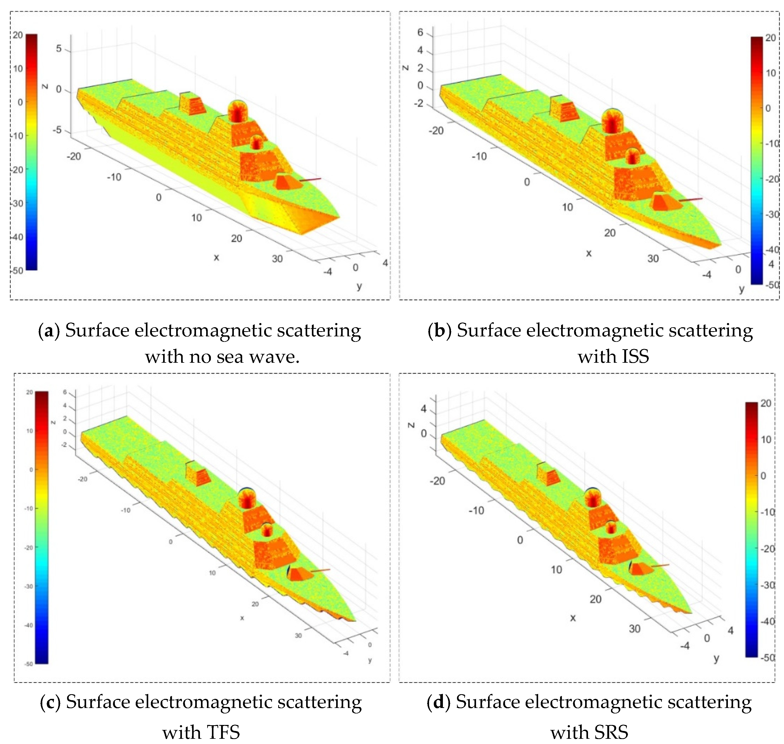
Figure 13 investigates the notion that the existence of ocean waves indeed affects the electromagnetic scattering characteristics of warship surfaces under the given observation conditions, where the following settings are made: θ(°) = −2sin t, γ(°) = 3sin t, As(°) = −1.5sin t, At(°) = 90sin t, α = 330°, β = 2°, t = 0.642 s, fR = 7 GHz, RCS unit: dBm2. When the sea wave model is not considered, all surface elements in the ZI1 area of the warship surface participate in the RCS contribution, where the azimuth is equal to 330° and the elevation angle is equal to 2°, causing most of the warship’s right and front areas to be illuminated by radar waves. Following this, a large area of deep red and red appeared on the right side of the turret, the front of the superstructure, the right front of the spherical radome and the front of the chimney. When the ideal stationary sea (ISS, as shown in Appendix A) wave model was added, where Zm = −2.1 m, xn = yn = −90 m, xm = ym = 90 m, the original ZI1 area was clearly cut out. Although there was no effect on the strong scattering area, the lighting zone changed significantly. Since there is no fluctuation in the wave model at this time, the cut in the surface electromagnetic scattering model of the warship is flat. When the trigonometric function sea (TFS, as shown in Appendix A) model is added, where Ax = 0.5, Ay = 0.2, ωx = ωy = 10, the notch of the warship electromagnetic scattering model is not flat, but changes with the waves. Since the TFS model is based on the trigonometric functions, taking into account linear variables, tiny random phases, and tiny random wave fluctuations, the edges of the cutout mainly show the undulating shape of the trigonometric function but with small irregular jitters. For the simplified regular sea (SRS, as shown in Appendix A) model, where k1 = 4, χ1 = π/3, χ0 = π/10, ω1 = Cz = 1, U = 10 m/s, it is also based on a trigonometric function, taking into account the small random wave increments, which makes the cutout very smooth overall.
Figure 14 demonstrates that the presence of sea waves has a non-negligible impact on the instant RCS under the omnidirectional angle of the warship, where β = 0°, t = 1.692 s, fR = 7 GHz. For Figure 14a, the addition of ISS waves caused some large changes in the original RCS-azimuth curve within the azimuth ranges of 82.5°~87.75° and 165.5°~178.5°. Although the average values of the two RCS curves are similar, 16.411 dBm2 (no sea wave) and 16.525 dBm2 (ISS), the RCS difference can exceed 8 dBm2 (α = 86.75°) or even 16 dBm2 (α = 176.5°), because the warships here have a stealth design and shallow draft, while the hull below the deck can reflect some of the radar waves well into the water, which results in similar RCS averages at all angles. The front shape of the warship uses an excellent stealth design, which greatly weakens the impact of the waves. The rear design of the warship is rough, and the portion submerged by the sea waves accounts for a large proportion of the entire projection area, which causes the waves in this direction to have a great impact. For Figure 14b here, the two RCS curves are almost coincident, except for some minimum values which include the RCS at α = 161.8°, 176.5°, and 263°. Both the TFS and SRS sea wave models dynamically change the submerged part of the warship, and can set sea waves with different amplitudes and phase changes.
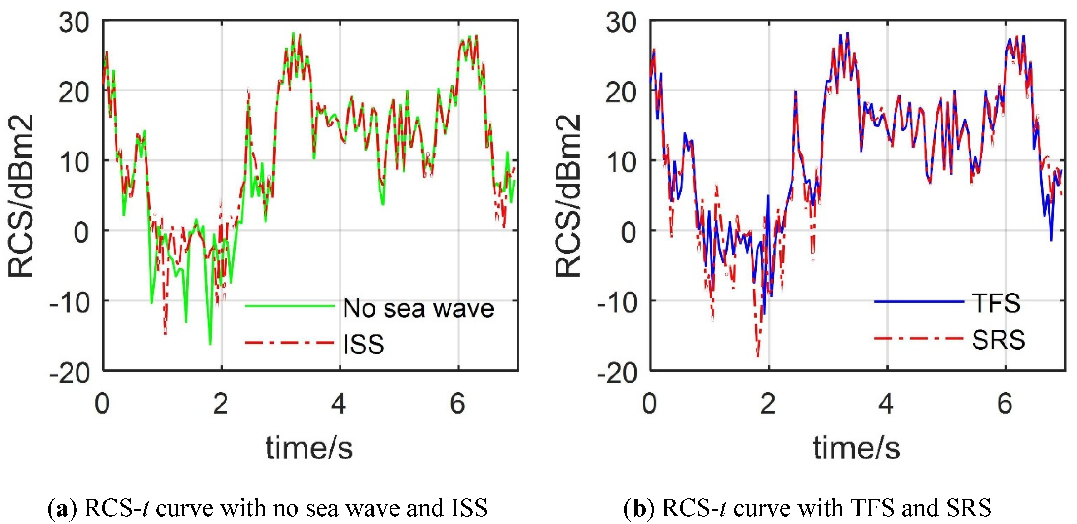
Figure 15 demonstrates that various ocean wave models have different effects on the dynamic electromagnetic scattering characteristics of warships under the given observation angles, where α = 85°, β = 0°, fR = 7 GHz. For Figure 15a here, the two RCS curves are generally similar and have large fluctuations. The maximum value of the RCS curve without the sea wave model exceeds 28 dBm2 at t = 3.325 s, and the minimum value is −16.34 dBm2 at t = 1.808 s, while the change in the warship RCS mainly comes from the real-time change in its attitude, although there are no sea waves. When the ISS wave model is added, the most obvious difference in RCS is reflected in the time range of [0.7583, 2.392] s when compared with the case without waves. At this time, the peak value of the RCS curve is 28.24 dBm2 appearing at t = 3.325 s, and the minimum value is −15.17 dBm2 at t = 1.05 s. The addition of the ISS wave model covers the lower part of the warship absolutely and uniformly in real time, which further affects the dynamic RCS of the warship when compared with the absence of waves. For Figure 15b here, the two RCS-time curves are also similar, except for some local fluctuations which are mainly reflected in the interval [0.233, 2.917] s. The minimum value of the RCS curve with the TFS wave model is −12 dBm2 at t = 1.925 s and the maximum value is 28.27 dBm2 at t = 3.325 s, while the other RCS curve has a peak value of 28.32 dBm2 and a minimum value below −18 dBm2. Both the TFS and SRS wave models are dynamic models that change with time and space, which causes the lighting area of warships to constantly change, while the trigonometric function structure, phase, amplitude, and random variables that make up the TFS and SRS models are different, which causes differences in their RCS-time curves. These results show that the DSA method can well capture the impact of wave models on warship RCS, including both the static and dynamic aspects.
In general, the sea wave model is a realistic factor that cannot be ignored when studying the electromagnetic scattering characteristics of warships. The presence of sea waves can change the attitude of warships, can affect the electromagnetic scattering area of warships, and, subsequently, can affect the radar cross-section of warships.
5. Conclusions
In this paper, we presents a dynamic scattering approach to solve the radar cross-section of the warship under complex motion conditions. Observation angle, turret rotation, attitude angle and wave model are considered and analyzed. Turret rotation brings significant changes to its average RCS and the RCS in all azimuths, but it has little effect on the average RCS of warships. The RCS-t characteristics of warships at different azimuth and elevation angles are very different. A slight increase in the elevation angle in the head-to-head direction can yield changes in the RCS average and peak position. The roll angle and pitch angle changes greatly affect the RCS-t curve of the warship at each azimuth angle. The sway angle has a greater impact on RCS-t than on RCS-α. The sea wave model has a significant impact on the RCS of warships in the lateral and tail directions. The stealth design of warship superstructure based on the dynamic RCS under important azimuth angles is one of the key development directions of future research.
Author Contributions
Conceptualization, Z.Z. and J.H.; methodology, software, validation, Z.Z.; formal analysis, Z.Z. and J.H.; investigation, writing—original draft preparation, writing—review and editing, funding acquisition, Z.Z. All authors have read and agreed to the published version of the manuscript.
Funding
This work was supported by the project funded by China Postdoctoral Science Foundation (Grant No. BX20200035).
Acknowledgments
Thanks to Professor Jun Huang for his guidance on the research work of this article.
Conflicts of Interest
The authors declare that there is no conflict of interest.
Nomenclature
| α | azimuth between the warship and the radar station [°] |
| β | elevation angle between the warship and the radar station [°] |
| θ | pitch angle of the warship [°] |
| γ | roll angle of the warship [°] |
| As | sway angle of the warship [°] |
| At | rotation angle of the gun turret [°] |
| t | time [s] |
| mtur | model of gun turret |
| mhul | model of warship hull after removing the turret |
| mwars | model of warship |
| Xtur | distance from zt axis to z axis [m] |
| M(mtur) | grid matrix of the turret model |
| M(mhul) | grid matrix of the hull model |
| M(mwars) | grid matrix of the warship model |
| zwave | sea wave surface function |
| σ | radar cross-section [dBm2] |
| ZI | the illuminated area of warship |
| ZD | the dark area of warship |
| NF | the number of facets |
| NE | the number of edges |
Subscript
| tur | gun turret |
| hul | warship hull |
| wars | warship |
| wave | sea wave |
Appendix A
When considering dynamic sea waves, the bins in ZI1 area need to be re-differentiated:
where F is the facet of the warship model in ZI1 area, Fu is the facet above the sea wave surface, and ZI is the illuminated area. Then, the facets below the waves can be defined as:
where ZD is the dark area. Other bins in ZI1 need to perform real-time median determination:
where Fm is the facet that intersects the sea wave surface, Z(Fu) indicates the area composed of all Fu facets, and Z(Fb) indicates the area composed of all Fb facets. Noting that:
Then, the model of the warship can be updated to the following form:
Using simple mathematical models to establish several real-time ocean wave geometries, the ideal stationary sea (ISS) wave model [36,37] is given as follows:
where Zm is a constant, which means that the sea is absolutely calm and does not change with space and time in the given range. A trigonometric function sea (TFS) wave model [28,37] is defined as:
where Ax, Ay, Ar, ωx and ωy are all custom constants, and r1, r2 and r3 are all random numbers in [0,1].
Appendix B
According to the magnetic vector position expression when the target is illuminated by radar waves, the electric field and the magnetic field can be respectively determined:
where ω is the electromagnetic wave angular frequency, k is the wave number in free space, R is the distance between the field point and the source point, Js is the induced current on the target surface, r′ is the coordinate vector of the source point, S is the target surface, and ε is the dielectric permittivity [15,18]. According to the association of physical optics, the dark and light areas can be distinguished as follows:
where n is the unit normal vector of the outer normal direction of r’ at the target surface. Based on the mirror principle:
For the case where the incident wave is a plane wave:
Then, there are the following expressions:
Considering the characteristics of plane waves, an integral term can be written as:
Then, the RCS calculation formula can be sorted into the following form:
PTD is used to solve the diffraction coefficient of the edge; then, the actual scattering field is the sum result of PO and PTD:
The diffraction coefficient of PTD can be expressed as:
where f1 is the diffraction coefficients of transverse magnetic waves of PTD, g1 is the diffraction coefficients of transverse electric waves of PTD, f is the diffraction coefficients of transverse magnetic waves of GTD, and g is the diffraction coefficients of transverse electric waves of GTD.
References
- Hopkins, B.; Miroshnichenko, A.E.; Poddubny, A.N.; Kivshar, Y.S. Fano resonance enhanced nonreciprocal absorption and scattering of light. Photonics 2015, 2, 745–757. [Google Scholar] [CrossRef]
- Feng, Y.; Zhu, W.; Huang, L.Y. Development and Assumption on Radar Stealth Technology of Surface Combat Ships. Ship Electron. Eng. 2018, 38, 5–8. [Google Scholar]
- Sun, B.; Yang, P.; Kattawar, G.W.; Zhang, X. Physical-geometric optics method for large size faceted particles. Opt. Express 2017, 25, 24044–24060. [Google Scholar] [CrossRef] [PubMed]
- Yang, D.Q.; Chang, S.Y. The characteristic cross-section method on the shape radar stealthy design of naval vessels. Shipbuild. China 2008, 49, 113–120. [Google Scholar]
- Bogatskaya, A.; Schegolev, A.; Klenov, N.; Popov, A. Generation of Coherent and Spatially Squeezed States of an Electromagnetic Beam in a Planar Inhomogeneous Dielectric Waveguide. Photonics 2019, 6, 84. [Google Scholar] [CrossRef] [Green Version]
- Xiao, F.; Li, Y.X.; Li, M. Radar Stealth Techniques of Surface Warship. Shipboard Electron. Countermeas. 2009, 32, 35–37. [Google Scholar]
- Yalçin, U. Scattering from a cylindrical reflector: Modified theory of physical optics solution. JOSA A 2007, 24, 502–506. [Google Scholar] [CrossRef]
- Xiong, Y.; Ye, H.; Umeda, T.; Mizoguchi, S.; Morifuji, M.; Kajii, H.; Maruta, A.; Kondow, M. Photonic Crystal Circular Defect (CirD) Laser. Photonics 2019, 6, 54. [Google Scholar] [CrossRef] [Green Version]
- Bettle, M.C.; Gerber, A.G.; Watt, G.D. Unsteady analysis of the six DOF motion of a buoyantly rising submarine. Comput. Fluids 2009, 38, 1833–1849. [Google Scholar] [CrossRef]
- Tsai, C.C.; Tai, W.T.; Hsu, W.; Hsiao, S.C. Step approximation of water wave scattering caused by tension-leg structures over uneven bottoms. Ocean Eng. 2018, 166, 208–225. [Google Scholar] [CrossRef]
- Liu, Z.Z. Stealth and Anti-Stealth Techniques of Ships Radar. Ship Electron. Eng. 2008, 28, 33–36. [Google Scholar]
- Kim, K.; Kim, J.H.; Cho, D.S. Radar cross section analysis of marine targets using a combining method of physical optics/geometric optics and a Monte-Carlo simulation. Ocean Eng. 2009, 36, 821–830. [Google Scholar] [CrossRef]
- Yang, D.Q.; Chang, S.Y. The theory and method for naval vessel shape optimal design considering the radar stealthy performance. Ship Sci. Technol. 2006, 28, 42–47. [Google Scholar]
- Yao, T.; Zhu, D.; Ben, D.; Pan, S. Distributed MIMO chaotic radar based on wavelength-division multiplexing technology. Opt. Lett. 2015, 40, 1631–1634. [Google Scholar] [CrossRef] [PubMed]
- Zhou, Z.Y.; Huang, J.; Yi, M.X. Comprehensive optimization of aerodynamic noise and radar stealth for helicopter rotor based on Pareto solution. Aerosp. Sci. Technol. 2018, 82, 607–619. [Google Scholar] [CrossRef]
- Shao, H.G. Application of radar stealth technology in surface ships. China Water Transp. 2017, 17, 79–80. [Google Scholar]
- Borovoi, A.; Grishin, I.; Naats, E.; Oppel, U. Backscattering peak of hexagonal ice columns and plates. Opt. Lett. 2000, 25, 1388–1390. [Google Scholar] [CrossRef]
- Zhou, Z.Y.; Huang, J.; Wu, N.N. Acoustic and radar integrated stealth design for ducted tail rotor based on comprehensive optimization method. Aerosp. Sci. Technol. 2019, 92, 244–257. [Google Scholar] [CrossRef]
- Sun, A.L.; Li, C.Q.; Liu, D.X.; Zhou, Y.H.; Dong, G.X. Study on Assessment of Shipping Water for Determination of Freeboard of Open-Top Containership. Shipbuild. China 2019, 60, 168–178. [Google Scholar]
- Surendran, S.; Lee, S.K.; Kim, S.Y. Studies on an algorithm to control the roll motion using active fins. Ocean Eng. 2007, 34, 542–551. [Google Scholar] [CrossRef]
- Zhao, Y.; Liu, J. FDTD for hydrodynamic electron fluid Maxwell equations. Photonics 2015, 2, 459–467. [Google Scholar] [CrossRef] [Green Version]
- de Tomasi, F.; Torsello, G.; Perrone, M.R. Water-vapor mixing-ratio measurements in the solar-blind region. Opt. Lett. 2000, 25, 686–688. [Google Scholar] [CrossRef]
- Chen, G.J.; Zhang, Z.; Mao, P. Research on U.S. Army Carrier Aircraft Approach Procedures and Standardized Design. Aviat. Stand. Qual. 2019, 5, 8–11,18. [Google Scholar]
- Vijayaraghavan, D.; Keith, T.G. Grid transformation and adaption techniques applied in the analysis of cavitated journal bearings. J. Tribol. 1990, 112, 52–59. [Google Scholar] [CrossRef]
- Zhou, Z.Y.; Huang, J. Target head direction far field radar cross section reduction based on narrow surface element method. Optik 2020, 200, 163230. [Google Scholar] [CrossRef]
- Bueno, L.C.; Borge, J.C.N.; Alexandre, E.; Hessner, K.; Sanz, S.S. Accurate estimation of significant wave height with support vector regression algorithms and marine radar images. Coast. Eng. 2016, 114, 233–243. [Google Scholar] [CrossRef]
- Zhao, J.; Lin, H. The engineering arithmetic of transforming grid coordinates into radar measure coordinates. Fire Control Command Control 2007, 32, 73–77. [Google Scholar]
- Memos, C.D.; Karambas, T.V.; Avgeris, I. Irregular wave transformation in the nearshore zone: Experimental investigations and comparison with a higher order Boussinesq model. Ocean Eng. 2005, 32, 1465–1485. [Google Scholar] [CrossRef]
- Zuo, X.S.; Wang, L.X.; Liu, H.L.; Wang, Y.; Zhang, Y. Research on similarity for simulating automatic carrier landing process of full-scale aircraft with scaled-model. Acta Aeronaut. Et Astronaut. Sin. 2019, 41, 123005. [Google Scholar]
- Ouyang, K.; Lin, R.K.; Wu, S.J.; Sheu, W.H. The Numerical Analysis of Flow Field on Warship Deck. Int. J. Eng. Res. 2015, 4, 118–122. [Google Scholar] [CrossRef]
- Mittapalli, V.; Khan, H. Excitation Schemes of Plasmonic Angular Ring Resonator-Based Band-Pass Filters Using a MIM Waveguide. Photonics 2019, 6, 41. [Google Scholar] [CrossRef] [Green Version]
- Ezhilsabareesh, K.; Suchithra, R.; Samad, A. Performance enhancement of an impulse turbine for OWC using grouped grey wolf optimizer based controller. Ocean Eng. 2019, 190, 106425. [Google Scholar] [CrossRef]
- Zhu, H.W.; Shao, Y.L.; Liu, Y.S. Chordal axis transformation based on mid-surface generation approach for thin-walled model. Comput. Integr. Manuf. Syst. 2018, 24, 649–659. [Google Scholar]
- Wu, P.F.; Shi, Z.S.; Wu, Z.H.; Hao, L.J. Estimation and Compensation Method of Deck Motion for Unmanned Helicopter Landing on Ship. Electron. Opt. Control 2019, 26, 22–27. [Google Scholar]
- Karam, M.A. Bridging the quasi-static and the physical optics approximations: An elliptic disk case. Appl. Opt. 1998, 37, 1666–1673. [Google Scholar] [CrossRef] [PubMed]
- Xiong, Y.F.; Shi, Z.G.; Guo, J.; Li, J.C. Sea Surface Modeling Based on the Spectrum of Ocean Waves Modeling and the FFT. J. Chongqing Univ. Technol. (Nat. Sci.) 2014, 28, 77–82. [Google Scholar]
- Pan, H.Y.; Zhao, J.C.; Wang, Z.L. Research on Modeling and Simulation of Virtual Sea Surface. Tonghua Teach. Coll. (Nat. Sci.) 2018, 39, 5–8. [Google Scholar]
- Aşırım, Ö.E.; Kuzuoğlu, M. Numerical study of resonant optical parametric amplification via gain factor optimization in dispersive microresonators. Photonics 2020, 7, 5. [Google Scholar] [CrossRef] [Green Version]
- Fei, C.J.; Wu, P.L.; Zhang, Q.Y.; Fang, G.Y.; Zhu, W.H. Improved Model of Ocean Wave Induced Magnetic Field Based on the First Order Stokes Equations. J. Electron. Inf. Technol. 2017, 39, 2007–2013. [Google Scholar]
- Liu, W.L.; Zhang, J. Optimization of the Wave Particle Mode Based on SPH by the MC Algorithm. J. Ocean Technol. 2017, 36, 41–45. [Google Scholar]
- Gao, L.; Reno, J.L.; Kumar, S. Short barriers for lowering current-density in terahertz quantum cascade lasers. Photonics 2020, 7, 7. [Google Scholar] [CrossRef] [Green Version]
Figure 1.
Schematic diagram of warship dynamic electromagnetic scattering.
Figure 2.
Triangular facets on the warship surface and the sea wave boundary.

Figure 3.
Verification of the dynamic RCS of the turret. (a) RCS-α curve; (b) RCS-t curve.

Figure 4.
Warship model and its main geometric size distribution.
Figure 5.
High-precision meshing of warship model surfaces.

Figure 6.
Electromagnetic scattering on the surface of the warship, RCS unit: dBm2. (a) Surface electromagnetic scattering; (b) Surface electromagnetic scattering under different azimuths and turret rotation.
Figure 6.
Electromagnetic scattering on the surface of the warship, RCS unit: dBm2. (a) Surface electromagnetic scattering; (b) Surface electromagnetic scattering under different azimuths and turret rotation.
Figure 7.
Dynamic radar cross-section of the single turret. (a) RCS-t curve; (b) RCS-t curve with large azimuth.
Figure 7.
Dynamic radar cross-section of the single turret. (a) RCS-t curve; (b) RCS-t curve with large azimuth.
Figure 8.
Impact of turret alone on the dynamic RCS. (a) Turret RCS-α curve; (b) Warship RCS-α curve.
Figure 8.
Impact of turret alone on the dynamic RCS. (a) Turret RCS-α curve; (b) Warship RCS-α curve.

Figure 9.
Effect of azimuth on the warship’s dynamic RCS. (a) RCS-t curve; (b) RCS-α curve.

Figure 10.
Effect of elevation angle on the warship’s dynamic RCS. (a) RCS-t curve; (b) RCS-α curve.
Figure 10.
Effect of elevation angle on the warship’s dynamic RCS. (a) RCS-t curve; (b) RCS-α curve.
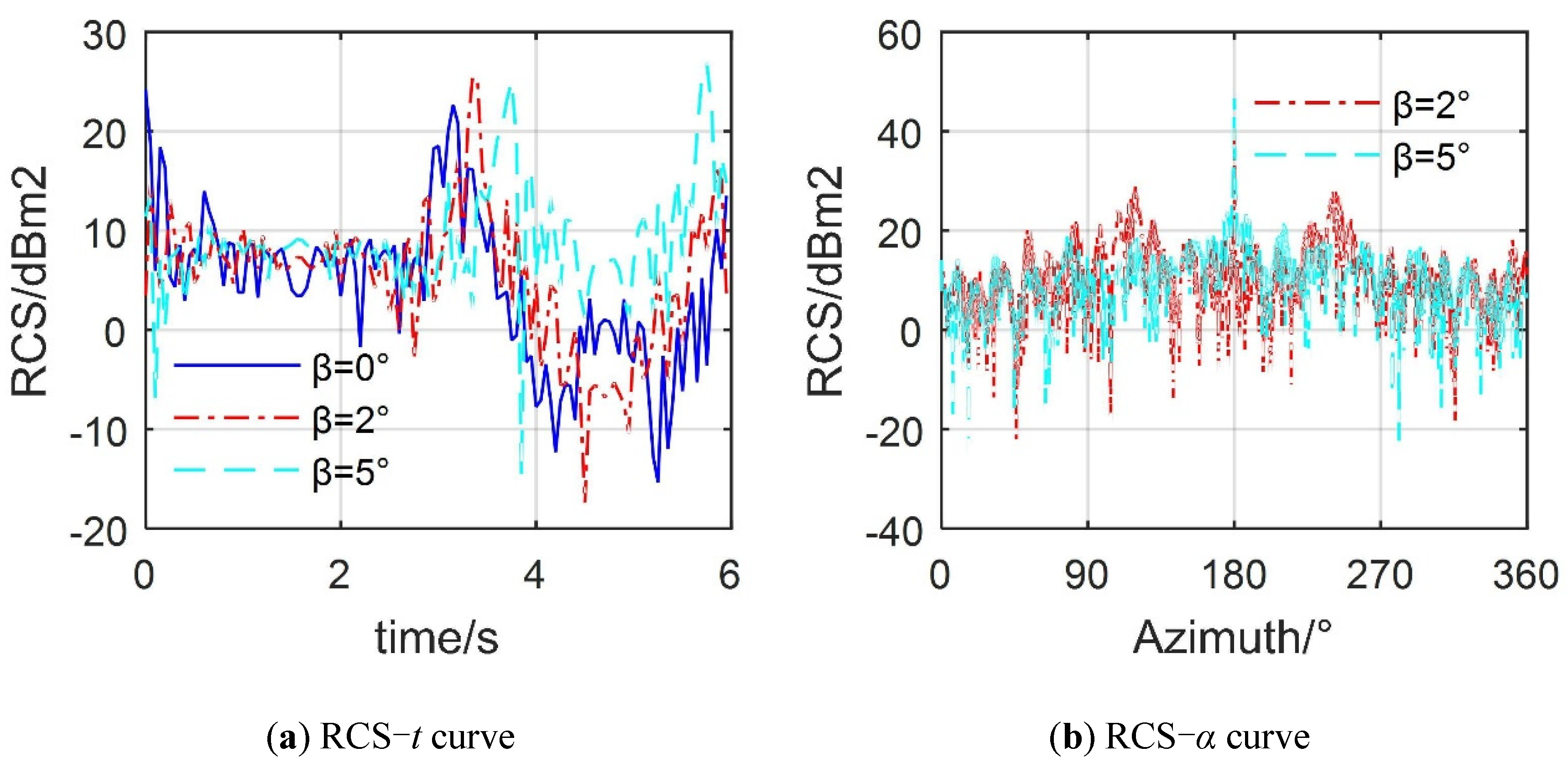
Figure 11.
Effect of attitude angles on the warship’s dynamic RCS. (a) RCS-t curve; (b) RCS-t curve at large azimuth.
Figure 11.
Effect of attitude angles on the warship’s dynamic RCS. (a) RCS-t curve; (b) RCS-t curve at large azimuth.
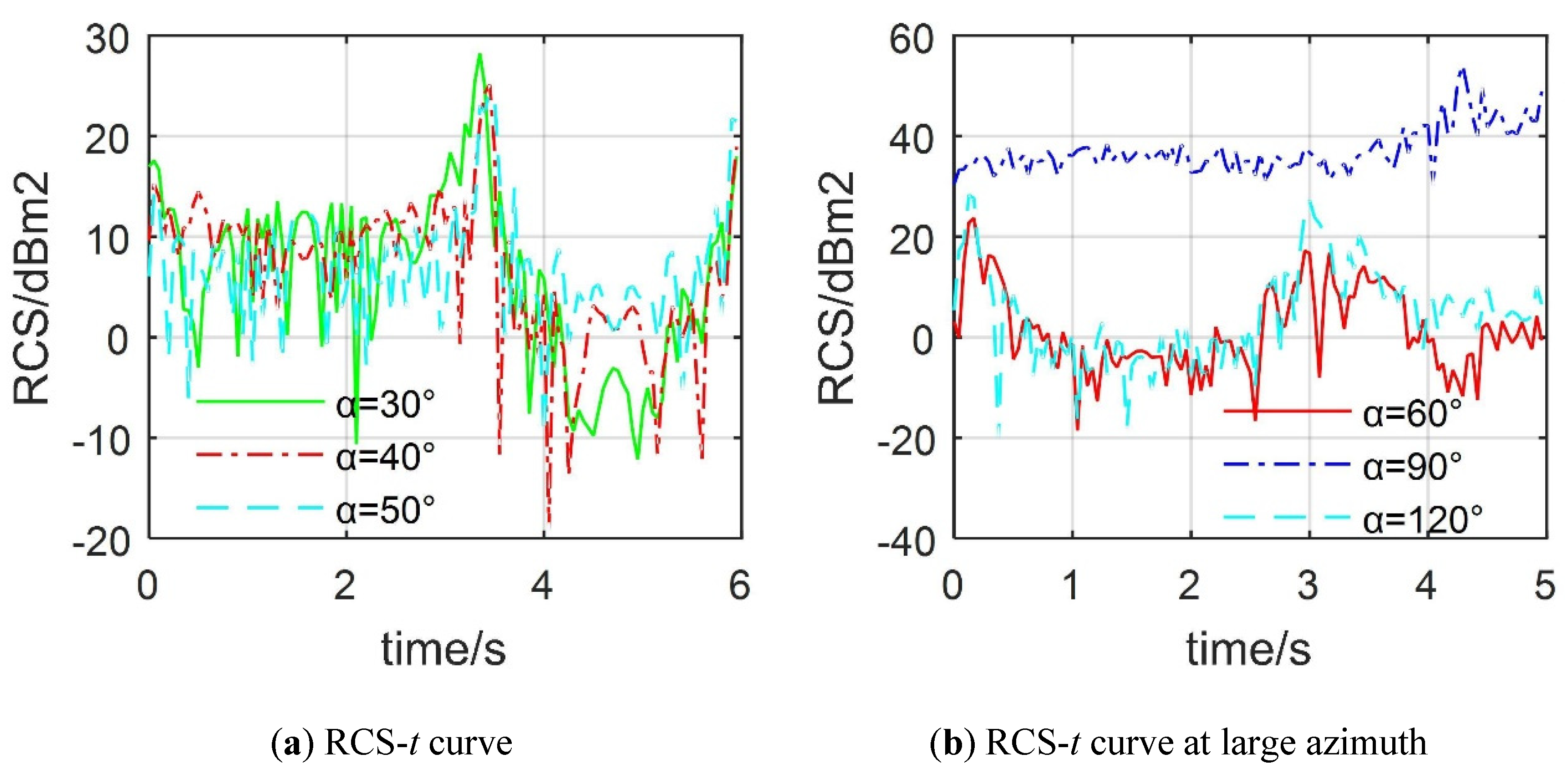
Figure 12.
Effect of attitude angles on the warship’s dynamic RCS. (a) RCS-t curve; (b) RCS-α curve.
Figure 12.
Effect of attitude angles on the warship’s dynamic RCS. (a) RCS-t curve; (b) RCS-α curve.

Figure 13.
Effects of different sea wave models on warship surface electromagnetic scattering. (a) Surface electromagnetic scattering with no sea wave; (b) Surface electromagnetic scattering with ISS; (c) Surface electromagnetic scattering with TFS; (d) Surface electromagnetic scattering with SRS.
Figure 13.
Effects of different sea wave models on warship surface electromagnetic scattering. (a) Surface electromagnetic scattering with no sea wave; (b) Surface electromagnetic scattering with ISS; (c) Surface electromagnetic scattering with TFS; (d) Surface electromagnetic scattering with SRS.

Figure 14.
Effects of different sea wave models on the warship’s RCS. (a) RCS-α curve with no sea wave and ISS; (b) RCS-α curve with TFS and SRS
Figure 14.
Effects of different sea wave models on the warship’s RCS. (a) RCS-α curve with no sea wave and ISS; (b) RCS-α curve with TFS and SRS
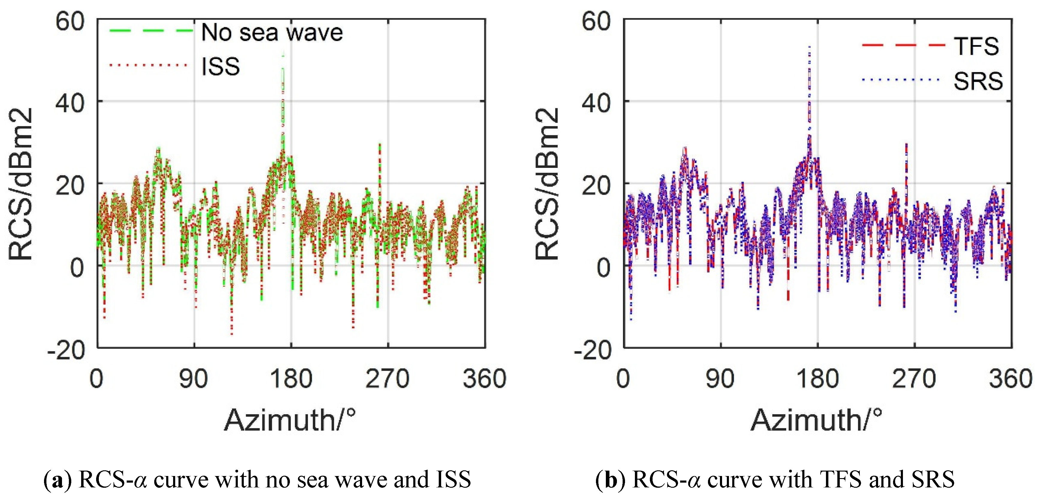
Figure 15.
Effects of different sea wave models on the warship’s dynamic RCS. (a) RCS-t curve with no sea wave and ISS; (b) RCS-t curve with TFS and SRS.
Figure 15.
Effects of different sea wave models on the warship’s dynamic RCS. (a) RCS-t curve with no sea wave and ISS; (b) RCS-t curve with TFS and SRS.

Table 1.
The main geometric dimensions of the warship model.
| Parameter | Lsh | L1 | L2 | L3 | L4 | L5 |
| Value/m | 60 | 19.5 | 8.74 | 11.7 | 9.95 | 10.11 |
| Parameter | Hsh | H1 | H2 | Wsh | Xt | |
| Value/m | 12.4 | 4.98 | 5 | 8 | 21.3 |
Table 2.
Grid size distribution on the surface of the warship model.
| Area | Maximum Value/mm | Area | Maximum Value/mm |
|---|---|---|---|
| Global minimum size | 3 | Gun barrel | 4 |
| Gun mount | 8 | Turret | 20 |
| Bow edge | 25 | Stern edge | 30 |
| Spherical radar | 30 | Chimney | 35 |
| Hull side ridge | 40 | Warship body | 50 |
© 2020 by the authors. Licensee MDPI, Basel, Switzerland. This article is an open access article distributed under the terms and conditions of the Creative Commons Attribution (CC BY) license (http://creativecommons.org/licenses/by/4.0/).
Share and Cite
MDPI and ACS Style
Zhou, Z.; Huang, J. Dynamic Scattering Approach for Solving the Radar Cross-Section of the Warship under Complex Motion Conditions. Photonics 2020, 7, 64. https://doi.org/10.3390/photonics7030064
AMA Style
Zhou Z, Huang J. Dynamic Scattering Approach for Solving the Radar Cross-Section of the Warship under Complex Motion Conditions. Photonics. 2020; 7(3):64. https://doi.org/10.3390/photonics7030064
Chicago/Turabian StyleZhou, Zeyang, and Jun Huang. 2020. "Dynamic Scattering Approach for Solving the Radar Cross-Section of the Warship under Complex Motion Conditions" Photonics 7, no. 3: 64. https://doi.org/10.3390/photonics7030064
Note that from the first issue of 2016, this journal uses article numbers instead of page numbers. See further details here.