Centroid Extraction Method Based on Multi-Scale Gaussian Fitting and Subpixel Edge Reconstruction

Abstract

Accurate spot-centroid localization is fundamental for determining optical metrics such as modulation transfer function (MTF) and effective focal length (EFL). Conventional methods struggle under non-ideal conditions—asymmetric spots, high noise, and vibration—and mid-wave infrared (MWIR) vibration has received little attention. To address these gaps, we propose multi-scale Gaussian fitting with subpixel edge reconstruction (MSGF-SER), combining image pyramid fitting, Zernike-moment edge extraction, and adaptive eccentricity-weighted fusion. Validated on simulated spots with varying SNRs and experimental sequences (visible off-axis aberration, long-wave infrared (LWIR) high-noise, MWIR micro-vibration), MSGF-SER achieved a noise-free RMSE of 0.03 pixel and 0.84 pixel at 5 dB SNR. On real MWIR vibration sequences, the Y-direction standard deviation (STD) dropped to 0.098 pixel, and the trajectory displacement variance was more than an order of magnitude lower than that of conventional methods. MTF deviations remained within 0.01, and the deviation of the measured mean EFL from the nominal focal length was better than 0.05 mm, and the STD was below 0.02 mm. These results demonstrate that MSGF-SER substantially improves centroid localization accuracy, repeatability, and smoothness under challenging conditions, providing reliable support for high-precision optical system parameter measurement.

1. Introduction

The imaging performance of high-precision optical industrial lenses sets the ultimate accuracy limit for precision inspection and metrology and thus is critical for advanced manufacturing and national defense applications [1,2,3,4]. A wide range of lens imaging parameters (MTF, EFL, wave aberration, etc.) must therefore be measured and calibrated to high quality, and the precision of spot-centroid localization directly constrains the accuracy of these parameter estimates. In aerospace optics, for example, ground calibration of star trackers depends critically on the centroiding accuracy of stellar spots: errors in centroid extraction propagate into focal-length and distortion estimates and thereby increase measurement uncertainty [5,6,7]. Similarly, in wavefront sensing, the Shack–Hartmann sensor relies on accurate localization of microlens-array spots; centroiding errors are a leading source of wavefront-reconstruction error [8,9,10]. In semiconductor manufacturing, subpixel localization of wafer alignment marks governs overlay precision in photolithography and thus demands robust centroid extraction algorithms [11,12,13]. Finally, in precision metrology systems that use laser-spot displacement to measure focal length, uncertainty in spot-center extraction likewise limits overall measurement accuracy [14,15,16]. Collectively, these examples illustrate that improving centroid localization—both in precision and robustness—is essential across diverse high-precision optical and metrology applications.

Although these applications arise in different contexts, they share an identical measurement chain: all extract centroid coordinates from spot images to infer optical parameters. Consequently, any small bias in centroid localization propagates through the calculation model and appears as an error in the measured parameters. The most widely used centroid extraction techniques are center of gravity (GC), ellipse fitting (EF), and Gaussian fitting (GF) [17,18,19,20,21]. The GC approach is computationally simple but vulnerable to spot asymmetry and high noise levels. EF derives the centroid from edge fitting, which makes it more adaptable to noncircular shapes; however, its performance hinges on accurate edge detection, and it is sensitive to outliers. GF models the intensity profile with a Gaussian function, which better represents many spot shapes and suppresses noise; accordingly, it currently affords the highest precision. Numerous refinements of GF have been proposed to tailor it to specific applications or to reduce its computational cost. Because Gaussian fitting is computationally intensive and struggles with real-time requirements, Wan et al. introduced a closed-form fast Gaussian fitting method that accelerates computation by roughly 15-fold [22]. Building on this approach, Yuan et al. combined Gaussian fitting with multi-scale convolution to enhance localization robustness at low signal-to-noise ratios [23]. Tang et al. demonstrated the applicability of Gaussian fitting in high-dynamic star sensors [24]. Nevertheless, most studies to date have targeted visible-light or space applications. Work specifically addressing centroid localization for mid-wave cooled infrared cameras operating in vibrating environments remains scarce. In such scenarios, spot degradation produces asymmetric shapes and blurred or partially corrupted edges; existing methods do not adequately exploit multi-scale information to cope with these challenges.

We propose a centroid extraction method that combines multi-scale Gaussian fitting with subpixel edge reconstruction to address these limitations. In the multi-scale Gaussian fitting stage, we construct an image pyramid and perform Gaussian fitting at each scale; a weighted fusion of the resulting estimates integrates multi-scale information, suppresses noise, and enhances subpixel localization accuracy. In the subpixel edge-reconstruction stage, we employ Zernike moments to recover subpixel coordinates of the spot edge and then refine the centroid via ellipse fitting, which enables robust accommodation of asymmetric spots and blurred edges. Overall, the method increases centroid localization accuracy and robustness while reducing computational overhead, thereby offering efficient and reliable technical support for high-precision measurement of critical optical parameters.

2. Centroid Extraction Method Based on Multi-Scale Gaussian Fitting and Subpixel Edge Reconstruction

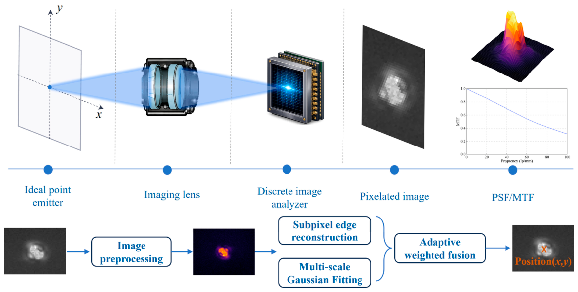
As shown in Figure 1, we propose a centroid extraction method, MSGF-SER, composed of three sequential modules: image preprocessing, multi-scale Gaussian fitting, and subpixel edge reconstruction. The first module prepares the raw spot image for reliable analysis by extracting a region of interest (ROI), converting it to grayscale, applying histogram equalization, and performing blob analysis. These steps suppress background noise and enhance the spot region for subsequent processing. The second module constructs an image pyramid and fits Gaussian models at each scale. Centroid estimates from individual scales are combined through a weighted fusion procedure to produce an initial centroid coordinate that leverages multi-scale information. The third module refines this initial estimate to subpixel accuracy. Subpixel edge coordinates are extracted using Zernike moments, and the centroid is then refined by ellipse fitting to the recovered edge points. This final refinement yields high-precision subpixel centroid coordinates.

2.1. Spot Image Preprocessing

Let the original grayscale image be I(x, y), with intensity levels in the range [0, L − 1] (for 8-bit images, L = 256). To reduce computational load and focus on the region containing the bright spot, a region of interest (ROI) is first extracted from the original grayscale image. For an arbitrary threshold T (0 ≤ T ≤ L − 1), the Otsu method is a fully automatic, parameter-free adaptive threshold segmentation technique that is particularly suitable for the bimodal histogram images in this study, where bright spots appear against a dark background. Its efficiency and stability have been validated in practical engineering applications; therefore, it is used to separate the image into foreground (pixels with gray values > T) and background (pixels with gray values ≤ T).

Let ${\omega }_0\left(T\right)$ and ${\omega }_1\left(T\right)$ denote the proportions of background and foreground pixels in the image, respectively, and let ${\mu }_0\left(T\right)$ and ${\mu }_1(T)$ denote the mean gray levels of the background and foreground, respectively. The between-class variance is then defined as:

$${\sigma }_b^2(T)={\omega }_0(T){\omega }_1(T){[{\mu }_0(T)-{\mu }_1(T)]}^2$$

(1)

Traverse all possible thresholds T using OTSU and select the threshold that maximizes the between-class variance as the optimal segmentation threshold:

$$T_{roi}=\arg \hspace{0.33em}\underset{0\le T\le L-1}{\max }({\sigma }_b^2(T))$$

(2)

Using this threshold to binarize the image yields the binary image B(x, y):

$$B(x,y)=\left\{\begin{array}{l}1,\hspace{0.33em}\hspace{0.33em}I(x,y)>T_{\mathrm{roi}}\\ 0,\hspace{0.33em}\hspace{0.33em}\mathrm{otherwise}\end{array}\right.$$

(3)

Then extract the bounding boxes of connected regions from the binary image as ROI regions ${\mathrm{\Omega }}_{\mathrm{ROI}}$ and perform subsequent processing only within the ROIs.

To enhance the contrast between the spot and the background, histogram equalization was applied to the ROI. Let the gray level be $r\in [0,L-1]$ and its probability density be $p_r(r)$; then the cumulative distribution function is:

$$s=T(r)=(L-1){\displaystyle \sum _{j=0}^r{p}_r(j)}$$

(4)

Map the original gray level r to a new gray level s to obtain the equalized image $I_{eq}(x,y)$:

$$I_{eq}(x,y)=T(I(x,y)),\hspace{1em}(x,y)\in {\mathrm{\Omega }}_{\mathrm{ROI}}$$

(5)

To avoid edge blurring, our method does not apply global filtering. Instead, we use Blob analysis (connected-component area filtering) to retain only the connected regions whose areas fall within a preset threshold range, thereby removing isolated small noise points without altering the spot shape. First, the equalized image was binarized again, with the threshold T recomputed by OTSU to obtain the binary image $B_{\mathrm{eq}}(x,y)$, where pixels with a value of 1 denote candidate spot regions.

Perform connected-component labeling on $B_{\mathrm{eq}}(x,y)$, with each connected component referred to as a blob. Let the pixel set of the k-th blob be $S_k$, and its area be $\left|S_k\right|$. Based on the physical dimensions of the spots, define an area threshold range $[A_{\min },A_{\max }]$, and retain only those blobs whose areas fall within this range:

$$S_k^{valid}=\left\{S_k\right|A_{\min }\le \left|S_k\right|\le A_{\max }\}$$

(6)

Because the target spot typically occupies the largest connected region, the blob with the greatest area is selected from the valid blobs as the final spot region S for subsequent centroid extraction.

$$S_{\mathrm{spot}}=\arg \underset{S_k^{\mathrm{valid}}}{\max }|S_k|$$

(7)

2.2. Multi-Scale Gaussian Fitting

To fully exploit spot information at multiple scales and enhance fitting robustness, a Gaussian pyramid of the spot image was constructed. The preprocessed spot image $I_0(x,y)$ (the grayscale image within the ROI) was used as level 0 of the pyramid. The image at level l was obtained by applying Gaussian filtering followed by downsampling to the image at level l − 1:

$$I_l(x,y)=\mathrm{downsample}(G_{\sigma }\ast I_{l-1}),\hspace{1em}l=1,2,\dots ,L$$

(8)

where $G_{\sigma }$ denotes the Gaussian low-pass filter with a standard deviation $\sigma$, typically set to 1.0; the downsampling factor is 2, i.e., the image dimensions are reduced by half at each level; the number of pyramid levels L is determined by the spot size, and in this study L = 3. This configuration ensures that the structural information of the spot is well preserved while enabling a coarse-to-fine multi-scale progressive refinement. It improves the stability of the initial centroid localization and achieves a good balance between computational efficiency and positioning accuracy.

At each scale l, the spot intensity distribution follows a two-dimensional Gaussian function:

$$f_l(x,y)=A_l\exp (-{\displaystyle \frac{{(x-x_{0,l})}^2}{2{\sigma }_{x,l}^2}}-{\displaystyle \frac{{(y-y_{0,l})}^2}{2{\sigma }_{y,l}^2}})$$

(9)

where $A_l$ denotes the peak intensity of the spot; $(x_{0,l},y_{0,l})$ denotes the coordinates of the centroid; and ${\sigma }_{x,l}$ and ${\sigma }_{y,l}$ denote the standard deviations in the x and y directions, respectively. Taking the natural logarithm of both sides of the above equation yields:

$$\ln f_l(x,y)=\ln A_l-{\displaystyle \frac{{(x-x_{0,l})}^2}{2{\sigma }_{x,l}^2}}-{\displaystyle \frac{{(y-y_{0,l})}^2}{2{\sigma }_{y,l}^2}}$$

(10)

Expanding and rearranging yields a quadratic form:

$$\ln f_l(x,y)=a_l{x}^2+b_l{y}^2+c_{l}x+d_{l}y+e_l$$

(11)

The relationships between the coefficients and the Gaussian parameters are given by:

$$a_l=-{\displaystyle \frac{1}{2{\sigma }_{x,l}^2}},b_l=-{\displaystyle \frac{1}{2{\sigma }_{y,l}^2}},c_l=-{\displaystyle \frac{x_{0,l}}{{\sigma }_{x,l}^2}},d_l=-{\displaystyle \frac{y_{0,l}}{{\sigma }_{y,l}^2}},e_l=\ln A_l-{\displaystyle \frac{x_{0,l}^2}{2{\sigma }_{x,l}^2}}-{\displaystyle \frac{y_{0,l}^2}{2{\sigma }_{y,l}^2}}$$

(12)

For an image on scale l, denoted I(x, y), take its logarithm to obtain $\ln I_l(x,y)$. Using the pixel coordinates as independent variables and (x, y) as the dependent variable, construct the following linear system of equations:

$$\ln I_l(x,y)=a_l{x}^2+b_l{y}^2+c_{l}x+d_{l}y+e_l+\epsilon$$

(13)

where $\epsilon$ denotes the fitting error.

Solve for the coefficient vector ${[a_l,b_l,c_l,d_l,e_l]}^T$ using the least squares method, and subsequently deduce the Gaussian parameters.

$$x_{0,l}=-{\displaystyle \frac{c_l}{2a_l}},\hspace{1em}{y}_{0,l}=-{\displaystyle \frac{d_l}{2b_l}}$$

(14)

Simultaneously, the fitting residual was computed to evaluate the goodness of fit at this scale. In this study, the root mean square error was used as the fitting residual $R_l$, defined as:

$$R_l=\sqrt{{\displaystyle \frac{1}{N_l}}{\displaystyle \sum _{i=1}^{N_l}{[\ln I_l(x_i,y_i)-(a_l{y}_i^2+b_l{y}_i^2+c_l{x}_i+d_l{y}_i+e_l)]}^2}}$$

(15)

where $N_l$ denotes the total number of pixels within the spot region; $I_l(x_i,y_i)$ represents the actual grayscale value of the l-th layer image at pixel $(x_i,y_i)$.

Map the centroid coordinates obtained from fitting images at different scales back to the original image scale. Denote the scaling factor of layer l relative to the original image as $2^l$; the mapped coordinates are:

$$x_{0,l}^{(0)}=2^l{x}_{0,l},\hspace{1em}{y}_{0,l}^{(0)}=2^l{y}_{0,l}$$

(16)

To combine multi-scale information ${\omega }_l$ we define a weight $R_l$ proportional to the fitting residual and also considering scale l (low-scale images contain rich detail but are noise sensitive; high-scale images are smoother but have lower resolution). In this paper, we compute the weight:

$${\omega }_l={\displaystyle \frac{1}{R_l(1+\alpha l)}}$$

(17)

where $\alpha$ is the scale penalization factor, typically set to 0.1. After normalization, the preliminary centroid of the weighted fusion is obtained:

$$x_{gauss}={\displaystyle \frac{{\displaystyle {\sum }_{l=0}^L{\omega }_l}{x}_{0,l}^{(0)}}{{\displaystyle {\sum }_{l=0}^L{\omega }_l}}},y_{gauss}={\displaystyle \frac{{\displaystyle {\sum }_{l=0}^L{\omega }_l}{y}_{0,l}^{(0)}}{{\displaystyle {\sum }_{l=0}^L{\omega }_l}}}$$

(18)

2.3. Subpixel Edge Reconstruction

Zernike moments map image grayscale information into the complex domain based on orthogonal polynomials; they possess orthogonality and rotational invariance and exhibit strong noise robustness. Therefore, this study employs Zernike moments for image edge extraction. For a continuous image $f(x,y)$, the Zernike moment of order n and repetition m is defined as:

$$Z_{nm}={\displaystyle \frac{n+1}{\pi }}{\displaystyle {\iint }_{x^2+u^2}f(x,y)}{V}_{nm}^{*}(\rho ,\theta )dxdy$$

(19)

where $V_{nm}(\rho ,\theta )=R_{nm}(\rho )e^{jm\theta }$ denotes a Zernike polynomial, $R_{nm}(\rho )$ denotes a radial polynomial, $(\rho ,\theta )$ denotes polar coordinates, and * indicates the complex conjugate.

Using the ideal edge model, within the unit circle, the edge divides the circle into two regions of grayscale values h and k, respectively. The distance from the edge to the circle center is l, and the angle between the edge normal and the x-axis is $\varphi$. The edge parameters l and $\varphi$ can be determined from three Zernike moments of different orders $Z_{00}$, $Z_{11}$ and $Z_{20}$.

Specifically, we first compute the rotated Zernike moment $Z_{nm}^{\prime }$ so that it aligns with the edge orientation. By exploiting rotational invariance, we have:

$$Z_{11}^{\prime }=Z_{11}{e}^{-j\varphi }$$

(20)

$$Z_{20}^{\prime }=Z_{20}$$

(21)

where $\varphi =\arctan \left({\displaystyle \frac{\mathrm{Im}[Z_{11}]}{\mathrm{Re}[Z_{11}]}}\right)$, the edge distance l can be determined from the real parts of $Z_{20}$ and $Z_{11}^{\prime }$:

$$l={\displaystyle \frac{Z_{20}}{Z_{11}^{\prime }}}$$

(22)

Since we have different templates and the image is Zernike moments at each pixel location, if 0 < l < 1 (the edge is in the unit circle), the pixels are edge points, and their subpixel coordinates are:

$$\left[\begin{array}{l}{x}_s\\ y_s\end{array}\right]=\left[\begin{array}{l}x\\ y\end{array}\right]+{\displaystyle \frac{N}{2}}l\left[\begin{array}{l}\cos \varphi \\ \sin \varphi \end{array}\right]$$

(23)

where N denotes the template size; in this study, it is set to 7 × 7. All edge points are extracted to form the point set $\epsilon =\{(x_i,y_i)\}$.

Perform a least-squares ellipse fit to the extracted subpixel edge points to obtain a more precise spot center. The general form of the ellipse equation is:

$$a{x}^2+b{y}^2+cxy+dx+ey+f=0$$

(24)

where a, b, c, d, e, f are the undetermined coefficients of the ellipse equation, subject to the ellipse constraint $4ab-c^2>0$. For each edge point $(x_i,y_i)$ substituted into the equation, a linear system is constructed:

$$\left[\begin{array}{cccccc}{x}_1^2& y_1^2& x_1{y}_1& x_1& y_1& 1\\ x_2^2& y_2^2& x_2{y}_2& x_2& y_2& 1\\ ⋮& ⋮& ⋮& ⋮& ⋮& ⋮\\ x_M^2& y_M^2& x_M{y}_M& x_M& y_M& 1\end{array}\right]\left[\begin{array}{l}a\\ b\\ c\\ d\\ e\\ f\end{array}\right]=0$$

(25)

The edge points used for ellipse fitting in this paper are derived from the candidate points satisfying 0 < l < 1 in the Zernike-moment subpixel detection results, which ensures the geometric reliability of the edge localization. Edge extraction is performed within the main spot region after ROI extraction and Blob analysis, where background noise and false targets have been removed. All subpixel edge points are used for ellipse fitting to fully exploit the contour information. Under the single-spot scenario, there is no multi-target interference, and the least-squares ellipse fitting is robust to local errors; therefore, no additional outlier removal strategy is introduced.

Solve the homogeneous system using the least-squares method to compute the ellipse parameters; the ellipse center obtained is taken as the fitted centroid coordinates:

$$x_{ellipse}={\displaystyle \frac{ce-2bd}{4ab-c^2}},\hspace{1em}{y}_{ellipse}={\displaystyle \frac{cd-2ae}{4ab-c^2}}$$

(26)

2.4. Adaptive Weighted Fusion Based on Spot Morphological Features

To better exploit geometric information of the light spot and to make the fusion weights more robust, we introduce an asymmetry factor derived from the ellipse’s eccentricity. We then map this factor to fusion weights using a saturating nonlinear transformation, which mitigates the susceptibility of conventional inverse-variance weighting to residual estimation errors.

First, based on the lengths of the semi-major axis a and semi-minor axis b (a ≥ b) obtained from the ellipse fitting procedure, the eccentricity e of the ellipse is defined as:

$$e=\sqrt{1-{\left({\displaystyle \frac{b}{a}}\right)}^2},\hspace{1em}e\in [0,1)$$

(27)

Let the asymmetry factor $\alpha =e^2=1-{\left({\displaystyle \frac{b}{a}}\right)}^2,\hspace{1em}\alpha \in [0,1)$, i.e., $\alpha =0$ corresponds to an ideal circular beam spot; a larger $\alpha$ indicates a more asymmetric beam shape.

Then, a sigmoid function is applied to $\alpha$ to perform a saturating nonlinear transformation, yielding the fusion weight $\beta$:

$$\beta ={\displaystyle \frac{1}{1+\exp (-k(\alpha -{\alpha }_0))}}$$

(28)

where k is the sensitivity coefficient that controls the steepness of the mapping curve; ${\alpha }_0$ is the offset parameter representing the threshold of asymmetry. The parameters were optimized by grid search on a simulated spot dataset using minimum root-mean-square error as the criterion, which yielded k = 8 and ${\alpha }_0=0.4$, corresponding to an eccentricity of $e=\sqrt{{\alpha }_0}\approx 0.63$.

Finally, the multi-scale Gaussian fitting results and the elliptical fitting results were fused to yield the final centroid coordinates:

$$x_{final}=\beta x_{ellipse}+(1-\beta )x_{gauss},\hspace{1em}{y}_{final}=\beta y_{ellipse}+(1-\beta )y_{gauss}$$

(29)

Specifically, the weighting coefficient $\beta$ decreases monotonically with increasing eccentricity. Consequently, the contribution of MSGF is dominant for near-circular spots, whereas the contribution of SER becomes dominant for asymmetric spots.

3. Experimental Validation and Results Analysis

3.1. Experimental System and Evaluation Metrics

We validated the centroid extraction approach—combining multi-scale Gaussian fitting with subpixel edge reconstruction—using both simulations and experiments on real spot images. The simulation studies quantified localization accuracy across a range of noise levels, while experiments with measured spot images evaluated the algorithm’s stability and practical performance under realistic imaging conditions. In addition, the method was applied to determine optical system parameters (MTF and EFL) to demonstrate its utility for improving optical measurements. For benchmarking, three standard centroid extraction algorithms served as comparisons: the GC method, the EF method, and the GF method. To enable a quantitative comparison of their performance, we used the following metrics.

RMSE was used to quantify the deviation between the estimated positions and the true centroid, and is defined as:

$$\mathrm{RMSE}=\sqrt{{\displaystyle \frac{1}{N}}{\displaystyle \sum _{i=1}^N[{(x_i-x_i^{true})}^2+{(y_i-y_i^{true})}^2]}}$$

(30)

where N denotes the number of test samples, $(x_i,y_i)$ represents the centroid coordinates extracted in the i-th instance, and $(x_i^{\mathrm{true}},y_i^{\mathrm{true}})$ denotes the true centroid coordinates.

Repeatability STD was used to assess the dispersion of multiple extraction results for the same static speckle target, reflecting the level of random error of the algorithm. It is defined as:

$$\mathrm{STD}=\sqrt{{\displaystyle \frac{1}{N-1}}{\displaystyle \sum _{i=1}^N{(x_i-\overline{x})}^2}}$$

(31)

where $\overline{x}$ denotes the mean of N computation results; a smaller STD value indicates better algorithmic repeatability.

Trajectory smoothness (TS) was used to assess the fluctuation magnitude of centroid displacements between consecutive frames, indirectly reflecting the algorithm’s capability to suppress vibrations. It is quantified by the variance of displacements between adjacent frames and is defined as:

$${\sigma }^2={\displaystyle \frac{1}{N-2}}{\displaystyle \sum _{i=1}^{N-1}{({\mathrm{\Delta }}_i-\overline{\mathrm{\Delta }})}^2}$$

(32)

where ${\mathrm{\Delta }}_i=\sqrt{{(x_{i+1}-x_i)}^2+{(y_{i+1}-y_i)}^2}$ denotes the centroid displacement between frame i and frame i + 1, and $\overline{\mathrm{\Delta }}$ represents the mean of ${\mathrm{\Delta }}_i$. A smaller ${\sigma }^2$ value indicates that the inter-frame displacement changes more smoothly, reflecting a higher trajectory smoothness of the algorithm.

3.2. Experiment on Centroid Extraction of Simulated Spot Images

We evaluated the algorithm using simulated circular Gaussian spots generated in MATLAB R2024a to represent ideal point sources. Each image measured 512 × 512 pixels, and the spot centroid was randomly positioned at (256.3, 256.7). To mimic realistic imaging conditions, we contaminated the simulations with an equal mixture of random Gaussian noise, shot noise, and salt-and-pepper noise (power ratio 1:1:1). Noise intensity was expressed as signal-to-noise ratio (SNR). For each SNR value of 5 dB, 10 dB, 15 dB, 20 dB, 25 dB, and ∞ (noise-free), fifty spot images were generated for each SNR level. The simulated spot images are shown in Figure 2.

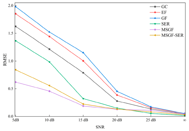
Figure 3 plots the localization RMSE for each method. All methods show decreasing RMSE as SNR increases. In the noiseless case, the proposed method (MSGF-SER) achieves an RMSE of 0.03 pixels, outperforming GC (0.04 pixels), EF (0.05 pixels), and GF (0.05 pixels). As SNR falls to 5 dB, the errors of the conventional methods rise sharply; by contrast, MSGF-SER maintains subpixel accuracy, with an RMSE of 0.84 pixels, demonstrating strong noise robustness.

To evaluate the execution efficiency of the proposed method, we conducted comparative experiments against conventional centroid extraction techniques and recorded the average processing time for a single 512 × 512 synthetic image. The results are presented in

Table 1. Comparison of average computation time for different centroid extraction methods.

Method	Average Computation Time (ms)
GC	0.422
EF	0.834
GF	0.826
MSGF	1.671

. The grayscale centroid method is the fastest, requiring only 0.422 ms; the elliptical fitting and Gaussian fitting methods have similar runtimes, approximately 0.83 ms; the proposed method, due to the construction of a three-level multi-scale pyramid and subpixel edge reconstruction using a 7 × 7 Zernike template, requires 1.671 ms, which is approximately four times that of the grayscale centroid method and twice that of the elliptical and Gaussian fitting methods.

Combining the data in Figure 3 shows that the proposed method significantly improves accuracy compared to conventional approaches. This enhancement comes with increased computational time, representing a trade-off between processing speed and precision. However, this trade-off allows for better management of complex scenarios and uncertainties, demonstrating greater robustness in practical applications. In engineering, high-precision data are essential for accurate decision-making. Therefore, the careful sacrifice of computation time to achieve more precise results holds substantial practical value in precision measurement applications.

3.3. Real Spot Image Centroid Extraction Experiment

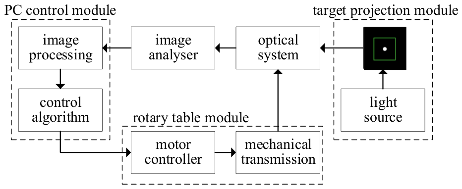
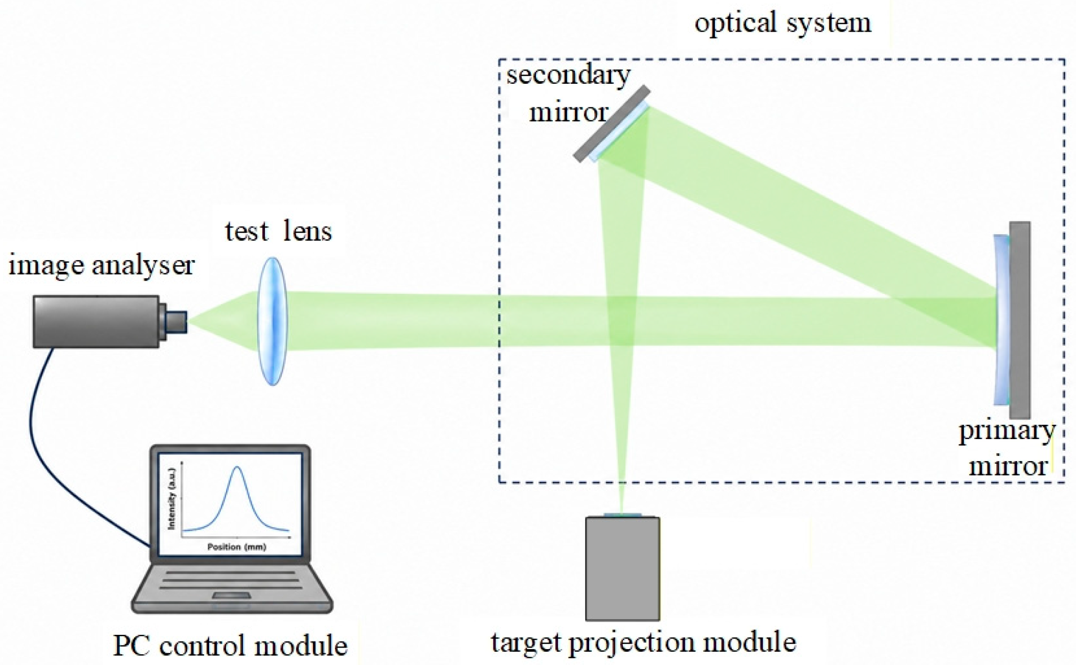
To validate the proposed method, we built an optical imaging experimental system; a schematic of its components appears in Figure 4. The system comprises five principal modules: the target generation module, the collimation optics, the image analyzer, the computation, processing and control module, and the rotation stage module. The target generator creates a star-point test pattern that the collimator renders into a collimated beam and projects onto the image analyzer’s sensor plane. The image analyzer captures these images in real time and relays them via a data interface to the computation, processing and control module. Simultaneously, the rotation stage is actuated to shift the target off the optical axis, intentionally distorting the imaged spot and thereby emulating noncircular spot morphologies.

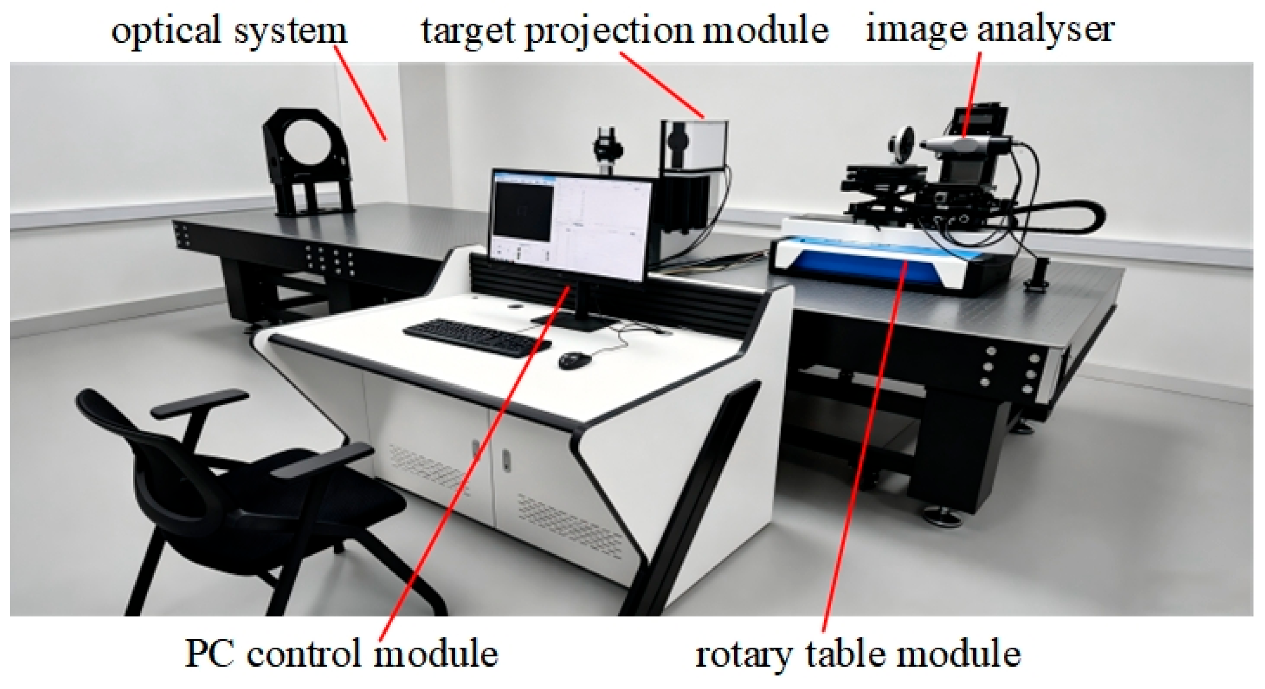
Figure 5 shows the experimental setup for centroid extraction of the optical system. The software runtime environment is CPU Intel^® Core™ i7-10700@2.9GHz (Intel, Santa Clara, CA, USA), RAM 32 GB, Qt 5.14.2. Figure 6 shows a schematic of the experimental platform, and

Table 2. Main component parameters of the experimental setup.

Component	Main Parameters
Target projection module	Star target size 0.2 mm, wavelength band 0.4 µm–12 µm
Optical system	Focal length 3000 mm, aperture 300 mm
Visible detector	1920 × 1200 pixels, pixel size 5.86 µm
MWIR detector	640 × 512 pixels, pixel size 15 µm, cooled
LWIR detector	640 × 512 pixels, pixel size 15 µm, uncooled
Rotary table module	Resolution 0.4″, positioning accuracy 3″
PC control module	OS Windows 10, CPU i7-10700, RAM 32 GB

summarizes the parameters of the principal components of the experimental system.

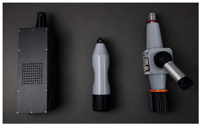
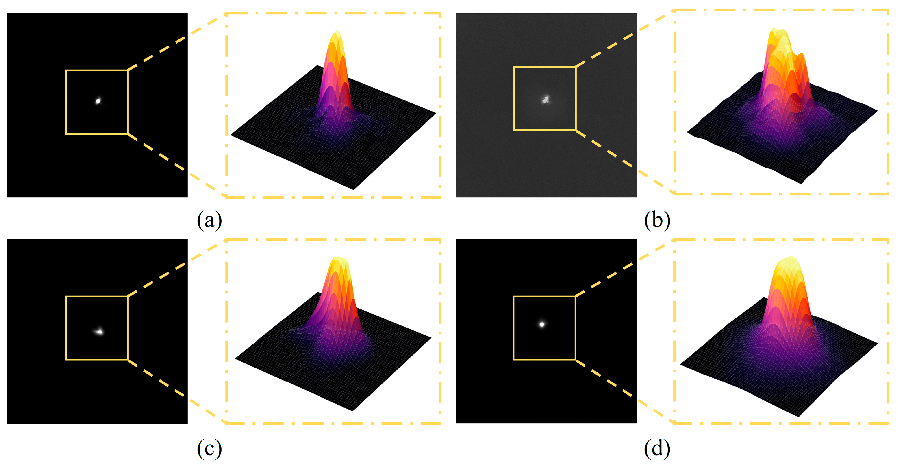
We evaluated the centroid extraction performance of the proposed method under varied imaging conditions using three standard lenses coupled to detectors with different spectral sensitivities; photographs of the devices are shown in Figure 7. The LWIR detector was uncooled and therefore produced very high imaging noise, whereas the mid-wave detector was Stirling-cooled and exhibited small spot vibrations in the frames. In contrast, the visible-light detector yielded high-quality images approximating ideal Gaussian spots. To induce asymmetric, noncircular spot shapes, we introduced an off-axis field by rotating the stage to create a 3° field offset. In total, four image sequences were acquired: 50 on-axis visible-band frames, 50 off-axis visible-band frames with a 3° field offset, 50 on-axis LWIR-band frames, and 50 on-axis mid-wave-band frames. Representative images for each condition are shown in Figure 8. The mid-wave and LWIR images have a resolution of 640 × 512 pixels, while the visible images are 1920 × 1200 pixels.

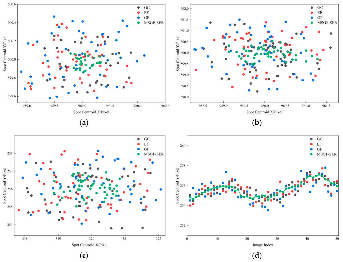
We extracted spot centroids from each frame of three static image sets—visible axis, off-visible axis, and LWIR band—using GC, EF, GF, and the proposed MSGF-SER method. For each technique, we computed the STD of the X and Y coordinates and generated 50-point scatter plots of the extracted centroids; the results are presented in Figure 9. Because spot positions and shapes are constant within each image set, observed centroid variations mainly reflect algorithmic stochastic errors and detector noise.

On-axis visible-light conditions: When spot morphology is highly symmetric and imaging noise is minimal, all methods reliably recover the centroid. Nonetheless, the MSGF-SER method yields a substantially smaller STD—0.10 pixels in X and Y—compared with GC (0.25/0.26 pixels), EF (0.28/0.30 pixels) and GF (0.31/0.32 pixels). Moreover, the intrinsic convergence behavior of MSGF-SER produces identical subpixel coordinates far more often under repeated processing of the same frame: 21 out of 50 independent extractions versus 8, 6 and 3 for GC, EF and GF, respectively. This higher frequency of identical outcomes—2.6, 3.5 and 7 times those of GC, EF and GF—demonstrates the exceptional numerical repeatability of MSGF-SER in ideal conditions and indicates that the combined multi-scale Gaussian fitting and subpixel edge reconstruction effectively suppress residual random error, driving repeated computations to converge to nearly the same location.

Visible off-axis distortion condition: Asymmetry in the spot shape markedly degrades the repeatability of conventional methods, yielding GC STDs of 0.87/0.92 pixels, EF of 1.18/0.98 pixels, and GF of 1.23/1.10 pixels. In contrast, MSGF-SER, which uses an adaptive weighted fusion strategy, preserves shape adaptability and reduces variability, with STDs of 0.41 pixels and 0.28 pixels in the X and Y directions, respectively.

Under LWIR, in high-noise conditions, all methods showed increased STDs. However, the X/Y STDs for MSGF-SER (0.88/0.92 pixels) remained roughly half to two-fifths of those for conventional approaches (GC: 1.65/1.78; EF: 1.69/1.84; GF: 2.03/2.16), demonstrating markedly greater noise resilience. These findings therefore confirm the proposed method’s high repeatability and robustness across different static imaging conditions.

Figure 9d presents the extracted centroids from 50 consecutive frames under MWIR vibration. Because the cooler-induced micro-vibrations primarily propagate along the image Y-axis, the analysis concentrates on the Y-coordinate variation produced by each method. Note that the true spot-center position is unavailable in these real vibration conditions; accordingly, this experiment aims to evaluate the relative positional stability of different algorithms in a vibrating environment rather than their absolute localization accuracy. Given the cooler’s fixed structural and frequency characteristics, the actual spot motion should be continuous and smooth; therefore, the random jitter and occasional jumps observed in the extracted trajectories are largely attributable to centroid extraction errors. Figure 9d shows that MSGF-SER produces the smallest fluctuations in the Y-direction centroid coordinates and the smoothest trajectory. By contrast, the Y-direction traces from GC, EF, and GF display pronounced random jitter and occasional jumps. Quantitatively, the standard deviation (STD) of MSGF-SER in Y is 0.098, markedly lower than GC (0.395), EF (0.548), and GF (0.657). When examining inter-frame displacement variance in Y only, MSGF-SER attains 0.0037—more than an order of magnitude smaller than GC (0.0312), EF (0.0458), and GF (0.0522)—indicating a substantially smoother and more stable centroid trajectory under vibration. These improvements in trajectory stability also translate into better optical measurements. As detailed in the MTF and EFL experiments (see Section 3.4), MSGF-SER produces an MTF curve closest to the theoretical prediction and exhibits the smallest EFL measurement error and best repeatability. Together, the trajectory statistics and measurement results confirm that MSGF-SER yields more stable and reliable centroid localization in complex MWIR operating conditions.

3.4. Optical-Parameter Measurement Experiments

MTF was measured using the star-point method. In this approach, the image-plane intensity distribution of a star-point target (the point spread function) is acquired, and a two-dimensional Fourier transform is applied to yield the modulus of the optical transfer function, i.e., the MTF curve. The procedure is as follows: locate the spot centroid, extract a subregion centered on that centroid, compute and normalize the two-dimensional Fourier transform, and then perform a radial averaging to obtain the MTF as a function of spatial frequency. The detailed calculation is provided in reference [25].

EFL was determined with the rotary-angle method. The lens under test is mounted on a high-precision rotary stage and rotated by a known angle ω while the displacement Δy (pixels) of the spot centroid on the image plane is recorded. The focal length is then calculated as f = Δy·d/tan(ω), where d is the pixel size. Detailed experimental procedures are given in reference [26].

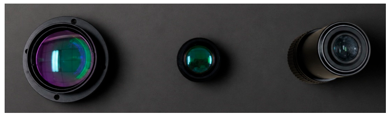
To assess how centroid extraction accuracy influences downstream optical-parameter measurements, we used the centroid coordinates obtained under the four test conditions described above to compute MTF and EFL. Experiments employed three standard lenses covering visible, MWIR, and LWIR bands; photographs of the physical devices appear in Figure 10, and their specifications are listed in

Table 3. Main parameters of the standard lens.

Parameter	Visible Lens	MWIR Lens	LWIR Lens
Wavelength Band (μm)	0.4–0.7	3–5	8–12
Focal Length (mm)	66.3	50	50
F-number	2.5	1.2	1.2

. When the visible-band spot is on-axis and otherwise ideal, image quality is high, and differences among centroid extraction methods have negligible impact on the resulting MTF and EFL. By contrast, under the three non-ideal conditions—visible-band off-axis distortion, elevated noise in the LWIR, and vibration in the MWIR—errors in centroid localization propagate through the analysis and measurably affect the computed MTF and EFL. The remainder of this section compares the accuracy of optical-parameter measurements obtained with our method to those produced by alternative centroid extraction approaches under these three challenging conditions. Detailed MTF and EFL results are reported in Section 3.4.1 and Section 3.4.2, respectively.

3.4.1. MTF Measurement Experiment

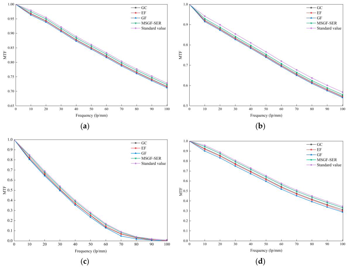
We evaluated how centroid extraction accuracy affects MTF measurements by performing tests in four representative configurations: on-axis visible, off-axis visible, LWIR, and MWIR. For each lens and spatial frequency, MTF values were computed using the star-field method. We then compared the proposed MSGF-SER centroiding algorithm with three conventional techniques: GC, EF, and GF. The theoretical MTF curves—generated by optical design software—served as benchmarks and correspond to a visible lens (66.3 mm focal length, F/2.5) and the MWIR and LWIR lenses (50 mm focal length, F/1.2).

Figure 11 shows the MTF curves measured by different methods under four typical conditions: on-axis visible ideal spots, off-axis visible distorted spots, long-wave infrared high-noise spots, and mid-wave infrared vibration spots. As shown in Figure 11a, under the on-axis visible ideal condition, all methods yield MTF curves that are in excellent agreement with the theoretical curve, with the maximum deviation being less than 0.005, indicating that centroid localization error has a negligible effect on MTF when the spot is ideal. However, under the off-axis visible distorted condition (Figure 11b), the spot exhibits an asymmetric shape. The MTF curves obtained by the GC, EF, and GF methods are notably lower than the theoretical curve in the mid-to-high frequency range (above 50 lp/mm), with maximum deviations of 0.036, 0.033, and 0.042, respectively. In contrast, the proposed MSGF-SER method, leveraging its adaptive fusion strategy, limits the full-band deviation to within 0.01, demonstrating excellent adaptability to asymmetric spots.

Under the LWIR high-noise condition (Figure 11c), the MTF curves of the GC, EF, and GF methods exhibit irregular fluctuations in the 30–70 lp/mm range, with maximum deviations of 0.045, 0.040, and 0.056, respectively, showing poor repeatability. The MSGF-SER method, however, maintains a smooth curve with a maximum deviation of only 0.009, indicating significantly better noise-suppression capability than the conventional methods. Under the MWIR vibration condition (Figure 11d), the Y-direction micro-vibration induced by the Stirling cooler causes periodic fluctuations in the MTF curves of the conventional methods in the 40–60 lp/mm range, with deviations of 0.032, 0.028, and 0.038 for GC, EF, and GF, respectively. Benefiting from the high smoothness of its centroid trajectory, the MSGF-SER method controls the full-band deviation within 0.008, verifying its excellent vibration suppression capability. In summary, the proposed method significantly improves MTF measurement accuracy under various challenging conditions, consistently limiting the deviation between the measured MTF and the theoretical value to within 0.01, thereby providing a reliable guarantee for the precise evaluation of the modulation transfer function of optical systems.

3.4.2. EFL Measurement Experiment

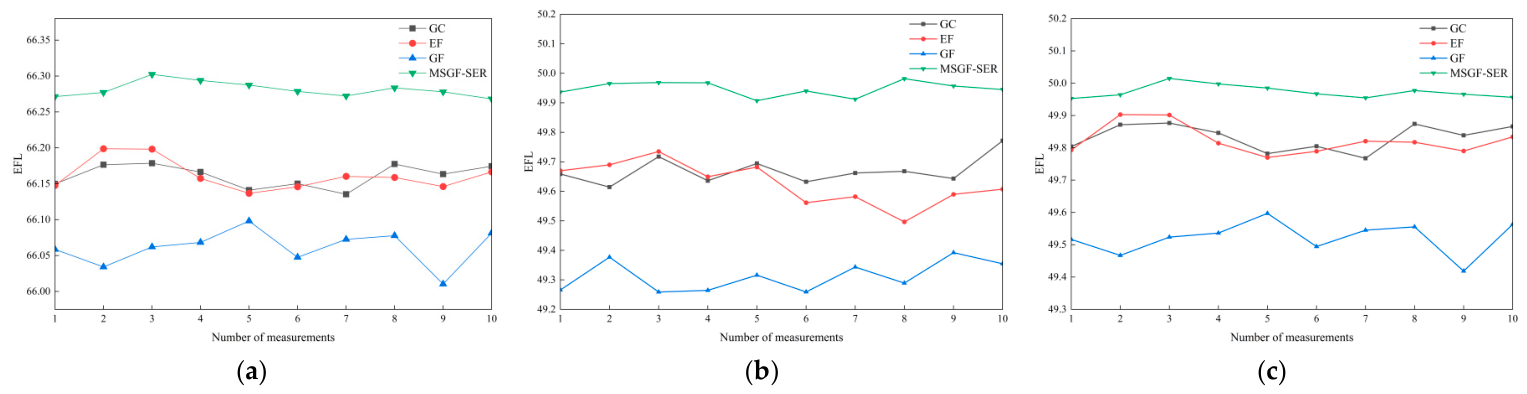
Because an ideal spot on the visible-light axis has negligible effect on focal-length measurements, we evaluated the proposed method under more realistic, non-ideal conditions by measuring the visible-light lens EFL with off-axis distortion. Centroid coordinates extracted from three scenarios—visible-light off-axis distortion, LWIR, and MWIR—were used separately to compute the EFL, allowing assessment of how centroid extraction accuracy influences effective focal length estimates. The resulting EFL values are plotted in Figure 12, and their means and STDs are reported in

Table 4. EFL measurement results using different centroid extraction methods.

Method	Visible Lens- Mean (mm)	MWIR Lens Mean (mm)	LWIR Lens- Mean (mm)	Visible Lens- STD (mm)	MWIR Lens- STD (mm)	LWIR Lens- STD (mm)
GC	66.16	49.83	49.66	0.019	0.048	0.052
EF	66.16	49.82	49.63	0.021	0.045	0.050
GF	66.07	49.54	49.31	0.028	0.057	0.060
MSGF	66.28	49.97	49.95	0.009	0.018	0.019

.

The EFL measurements across the three operating conditions show notable differences in accuracy and robustness among the tested methods. Under off-axis visible-light distortion (nominal focal length 66.30 mm), the conventional GC and EF methods produced mean focal lengths of 66.16 mm, while the GF method yielded 66.07 mm; their STDs ranged from 0.019 to 0.028 mm. The GF method showed the largest bias from nominal, 0.23 mm. By contrast, the proposed MSGF-SER method returned a mean of 66.28 mm—only 0.02 mm from nominal—with a STD of 0.009 mm, roughly one-half to one-third that of the conventional approaches, indicating markedly improved shape adaptability. Under high-noise LWIR conditions (nominal focal length 50.00 mm), noise markedly increased the measurement bias of conventional methods: GC, EF, and GF deviated from the nominal value by 0.34 mm, 0.37 mm, and 0.69 mm, respectively. In contrast, MSGF-SER limited the deviation to 0.05 mm and produced an STD of 0.019 mm—approximately one-third that of the conventional approaches. Similarly, under MWIR vibration conditions (nominal focal length 50.00 mm), conventional methods suffered large fluctuations driven by Y-direction centroid jitter; the GF method alone showed a 0.46 mm deviation from the nominal value. By comparison, MSGF-SER produced a smooth centroid trajectory that constrained the deviation to 0.03 mm and yielded a STD of only 0.018 mm, substantially outperforming the conventional techniques. In summary, the method presented in this study markedly improves the accuracy and repeatability of EFL measurements under complex operating conditions. Across all tests, the deviation of the measured mean from the nominal focal length was better than 0.05 mm (relative deviation better than 2‰), and the repeatability STD was below 0.02 mm, fully validating the critical supporting role of high-precision centroid localization for focal length measurement.

4. Discussion

The results demonstrate that a single centroid extraction method cannot simultaneously provide strong shape adaptability, noise robustness, and vibration resistance under complex imaging conditions. By combining intensity-distribution information with geometric boundary information, the proposed MSGF-SER method effectively improves localization accuracy in degraded scenarios. While all methods perform well under ideal spot conditions, conventional approaches exhibit noticeable performance degradation in the presence of off-axis distortion, strong noise, and micro-vibrations. In contrast, MSGF-SER achieves stable initial estimation through multi-scale Gaussian fitting and further refines the centroid using subpixel edge reconstruction, resulting in superior accuracy and stability across different operating conditions.

Existing centroid localization methods generally fall into two categories: intensity-model-based approaches and geometry-based approaches. The former usually offers good noise resistance, whereas the latter is more suitable for non-ideal spot shapes. However, neither category alone can maintain consistent performance under varying imaging conditions. By integrating these complementary sources of information, the proposed method improves adaptability to both spot deformation and environmental disturbances. The newly added ablation study further confirms that both multi-scale Gaussian fitting and subpixel edge reconstruction contribute positively to the final localization performance, validating the effectiveness of the proposed framework. Furthermore, the MTF and EFL experiments further indicate that improvements in centroid localization accuracy directly translate into more accurate and repeatable optical-parameter measurements. Under distortion, noise, and vibration conditions, centroid estimation errors propagate into subsequent MTF and focal-length calculations. By reducing such errors, MSGF-SER provides more stable measurement results and improves the overall reliability of optical metrology systems.

Although the proposed method demonstrates strong robustness in the investigated scenarios, its performance under more challenging conditions, such as overlapping spots, severe occlusion, and extremely low signal-to-noise ratios, remains to be studied. Future work will focus on combining data-driven techniques with physics-based constraints to further improve generalization capability and extend the method to applications such as star sensor calibration, adaptive optics, and semiconductor optical metrology.

5. Conclusions

This paper addresses limitations in centroid extraction for optical spots under degraded conditions—such as asymmetry, high noise, and vibration—common in high-precision optical measurements. We propose a centroid extraction method that combines multi-scale Gaussian fitting with subpixel edge reconstruction. After standard image preprocessing, the method builds a Gaussian pyramid to fuse multi-scale information and obtain an initial centroid estimate. It then extracts subpixel edges via Zernike moments, applies elliptical fitting for geometric correction, and integrates the Gaussian and edge-derived information using adaptive weights determined by spot eccentricity. We validate MSGF-SER using simulations and multi-spectral, multi-condition experiments on real spots. Compared with intensity-weighted centroid, elliptical fitting, and single-scale Gaussian fitting, MSGF-SER offers clear improvements in localization accuracy, repeatability, and trajectory smoothness. Under ideal conditions, the RMSE is 0.03 pixels. Under MWIR cryocooler vibration, the variance of trajectory displacement in the Y direction is 0.0037, indicating strong suppression of micro-vibrations induced by Stirling coolers. Applied to MTF and EFL measurements, MSGF-SER confines MTF bias to within 0.01 and yields an EFL measurement accuracy with a mean deviation < 0.05 mm and a repeatability STD < 0.02 mm, satisfying engineering metrology requirements. In summary, MSGF-SER delivers a robust, reliable subpixel localization approach for measuring critical optical system parameters under challenging conditions. Its demonstrated accuracy and stability make it well suited for precision inspection, aerospace optics, and semiconductor-manufacturing applications.

References

1. Pu, D.; Tao, H.; Ge, Y.; Liu, C.; Zhu, J. Improvements on Sampling of Point Spread Function in Optical Transfer Function Measurement. Opt. Express 2022, 30, 10953. [Google Scholar] [CrossRef] [PubMed]
2. Shimizu, Y.; Chen, L.-C.; Kim, D.W.; Chen, X.; Li, X.; Matsukuma, H. An Insight into Optical Metrology in Manufacturing. Meas. Sci. Technol. 2021, 32, 042003. [Google Scholar] [CrossRef]
3. Gao, W.; Haitjema, H.; Fang, F.Z.; Leach, R.K.; Cheung, C.F.; Savio, E.; Linares, J.M. On-Machine and in-Process Surface Metrology for Precision Manufacturing. CIRP Ann. 2019, 68, 843–866. [Google Scholar] [CrossRef]
4. Fang, Z.; Song, Y.; Han, B.; Wang, A.; Song, J.; Yue, H. Autofocusing Method Based on Dynamic Modulation Transfer Function Feedback. Photonics 2026, 13, 107. [Google Scholar] [CrossRef]
5. Wei, X.; Zhang, G.; Fan, Q.; Jiang, J.; Li, J. Star Sensor Calibration Based on Integrated Modelling with Intrinsic and Extrinsic Parameters. Measurement 2014, 55, 117–125. [Google Scholar] [CrossRef]
6. Tan, W.; Dai, D.; Wu, W.; Wang, X.; Qin, S. A Comprehensive Calibration Method for a Star Tracker and Gyroscope Units Integrated System. Sensors 2018, 18, 3106. [Google Scholar] [CrossRef] [PubMed]
7. Niu, Y.; Wei, X.; Li, J. Star Image Registration Modeling and Parameter Calibration for a 3CMOS Star Sensor. Sensors 2024, 24, 259. [Google Scholar] [CrossRef] [PubMed]
8. Vargas, J.; Restrepo, R.; Estrada, J.C.; Sorzano, C.O.S.; Du, Y.-Z.; Carazo, J.M. Shack–Hartmann Centroid Detection Using the Spiral Phase Transform. Appl. Opt. 2012, 51, 7362. [Google Scholar] [CrossRef] [PubMed]
9. Xiang, C.; Cheng, T.; Wang, Y.; Guan, H.; Ge, X.; Gao, Z.; Wang, S.; Yang, P. A Highly Adaptive Centroid Positioning Method for Shack-Hartmann Wavefront Sensor Based on Lightweight Object Detection Network. Opt. Laser Technol. 2025, 191, 113314. [Google Scholar] [CrossRef]
10. Gu, D.; Liu, X. Shack–Hartmann Wavefront Sensor Based on Kalman Filter. Opt. Eng. 2022, 61, 093106. [Google Scholar] [CrossRef]
11. Tang, Q.; Huang, X.; Miao, Y.; Huang, J. A Robust Algorithm for Rapid Pre-Alignment of Multiple Types and Sizes of Wafers. SIViP 2024, 18, 2559–2569. [Google Scholar] [CrossRef]
12. Pan, S.; Wang, S.; Xu, J.; Fan, L.; Yuan, F.; Shu, T.; Dai, F.; Yan, X.; Bu, Y.; Wang, X. Sub-Pixel Position Estimation Algorithm Based on Gaussian Fitting and Sampling Theorem Interpolation for Wafer Alignment. Appl. Opt. 2021, 60, 9607. [Google Scholar] [CrossRef] [PubMed]
13. Li, Y.; Cao, Y.; Li, S.; Tian, H.; Qi, G.; Wei, R. Subpixel Keypoint Localization and Angle Prediction for Lithography Marks Based on Deep Learning. J. Intell. Manuf. 2025, 36, 3843–3868. [Google Scholar] [CrossRef]
14. Gao, R.; Zhao, M.; Liu, H.; Qi, K.; Wang, S.; Li, P.; Wang, J.; Shen, J.; Luo, Z. Analysis of Laser Spot Centroiding Errors for Laser Acquisition System in Gravitational Wave Detection Missions. Opt. Express 2024, 32, 48556. [Google Scholar] [CrossRef] [PubMed]
15. Shen, L.; Guo, K.; Zhou, Q.; Li, X.; Sun, H.; Deng, Z.; Zhang, S.; Long, J. A Novel Laser Spot Centroid Positioning Method Based on Variable-Coefficient Error Compensation. Opt. Laser Technol. 2026, 194, 114468. [Google Scholar] [CrossRef]
16. Sun, J.; Xie, Y. Subpixel Spot Localization Using Multiscale Anisotropic Gaussian Tensor. Measurement 2023, 214, 112756. [Google Scholar] [CrossRef]
17. Zhang, Y.; Jiang, J.; Zhang, G.; Lu, Y. Accurate and Robust Synchronous Extraction Algorithm for Star Centroid and Nearby Celestial Body Edge. IEEE Access 2019, 7, 126742–126752. [Google Scholar] [CrossRef]
18. Delabie, T.; Schutter, J.D.; Vandenbussche, B. An Accurate and Efficient Gaussian Fit Centroiding Algorithm for Star Trackers. J. Astronaut. Sci. 2014, 61, 60–84. [Google Scholar] [CrossRef]
19. Wang, H.; Xu, E.; Li, Z.; Li, J.; Qin, T. Gaussian Analytic Centroiding Method of Star Image of Star Tracker. Adv. Space Res. 2015, 56, 2196–2205. [Google Scholar] [CrossRef]
20. Wang, F.; Zhu, Z.; Yan, H.; Qian, C.; Cai, B.; Yao, Y. Target Center Extraction Method Based on Joint Calibration of Camera and Radar. In Proceedings of the 2024 8th International Conference on Electronic Information Technology and Computer Engineering, Haikou Guangdong, China, 18–20 October 2024; ACM: New York, NY, USA, 2024; pp. 383–390. [Google Scholar]
21. Sun, G.; Qiao, Y.; Chen, W. A Grayscale Centroid Iterative Algorithm That Enables Parallel Extraction of the Position and Shape Information of the Light Spot. In Proceedings of the International Conference on Precision Instruments and Optical Engineering (PIOE 2025), Changsha, China, 8–10 October 2025; Guo, J., Xu, Z., Eds.; SPIE: Washington, DC, USA, 2025; p. 15. [Google Scholar]
22. Wan, X.; Wang, G.; Wei, X.; Li, J.; Zhang, G. Star Centroiding Based on Fast Gaussian Fitting for Star Sensors. Sensors 2018, 18, 2836. [Google Scholar] [CrossRef] [PubMed]
23. Yuan, K.; Li, L. Optimization of Laser Spot Edge Extraction and Localization Based on Multi-Scale Adaptive Convolution. Front. Phys. 2025, 13, 1650714. [Google Scholar] [CrossRef]
24. Tang, X.; Cao, Q.; Fu, Z.; Xu, T.; Duan, R.; Yang, X. Multi-Centroid Extraction Method for High-Dynamic Star Sensors Based on Projection Distribution of Star Trail. Remote Sens. 2025, 17, 266. [Google Scholar] [CrossRef]
25. Yilmaz, O.; Selimoglu, O. MTF Measurement of a SWIR Imaging Telescope Using Star Test Images. AIP Conf. Proc. 2012, 1476, 131–135. [Google Scholar] [CrossRef]
26. Zhou, X.; Liu, D.; Zhang, Z.; Cao, R.; Li, X.; Gu, X. Research on Focal Length Measurement of Telephoto Lens Based on Polaris Observation. In Proceedings of the AOPC 2020: Telescopes, Space Optics, and Instrumentation, Beijing, China, 30 November–2 December 2020; Zhang, Z., Xue, S., Eds.; SPIE: Washington, DC, USA, 2020; p. 21. [Google Scholar]
Figure 1. Spot-centroid localization system and algorithm workflow based on multi-scale Gaussian fitting and subpixel edge reconstruction.
Photonics 13 00594 g001
Figure 2. Simulated spot images under different SNRs: (a) SNR = 5 dB; (b) SNR = 10 dB; (c) SNR = 15 dB; (d) SNR = 20 dB; (e) SNR = 25 dB; (f) SNR = ∞.
Photonics 13 00594 g002
Figure 3. RMSE versus SNR curves for different centroid extraction methods.
Photonics 13 00594 g003
Figure 4. Schematic diagram of the optical system centroid extraction experimental setup.
Photonics 13 00594 g004
Figure 5. Optical system centroid extraction experimental setup.
Photonics 13 00594 g005
Figure 6. Schematic diagram of the optical system centroid extraction experimental platform.
Photonics 13 00594 g006
Figure 7. Photograph of the detector. From left to right: MWIR detector, LWIR detector, and Visible detector.
Photonics 13 00594 g007
Figure 8. Spot images under different operating conditions: (a) on the visible axis; (b) 3° off the visible axis; (c) on the long-wave axis; (d) on the mid-wave axis.
Photonics 13 00594 g008
Figure 9. Spot-centroid extraction results: (a) on the visible axis; (b) 3° off the visible axis; (c) on the long-wave axis; (d) on the mid-wave axis.
Photonics 13 00594 g009
Figure 10. Photograph of the standard lens assembly. From left to right: MWIR lens, LWIR lens, and Visible lens.
Photonics 13 00594 g010
Figure 11. MTF measurement accuracy under different algorithms: (a) visible lens on-axis; (b) visible lens off-axis; (c) LWIR lens; (d) MWIR lens.
Photonics 13 00594 g011
Figure 12. EFL measurement accuracy under different algorithms: (a) visible lens; (b) LWIR lens; (c) MWIR lens.
Photonics 13 00594 g012