Interpretable Microwave Sensing Using E-Band Commercial Links: Physics-Aware Deep Learning for Rainfall Detection

Abstract

Accurate rainfall monitoring is vital for hydrology and environmental sensing. This study presents a physics-aware deep learning framework using E-band (71–86 GHz) commercial microwave links (CMLs). Using the extensive urban CML dataset and methodology, a bi-directional Long Short-Term Memory (Bi-LSTM) model is developed to classify wet and dry periods under a temporal generalization framework across heterogeneous link configurations. The approach integrates physical signal decomposition, including baseline estimation, gaseous attenuation correction, and wet antenna attenuation (WAA) modeling, with sequence-based learning. Results demonstrate that the temporal deep learning model outperforms classical threshold-based and physical k–R approaches when evaluated over independent temporal validation blocks, effectively reducing sensitivity to path-length-related variability on heterogeneous paths. The model maintains stable performance (loss < 3%) under moderate signal-level noise. SHapley Additive exPlanations (SHAP) confirm the model relies on physical features, such as signal volatility and temporal trends, to reliably differentiate rainfall from WAA. This framework highlights the potential of E-band infrastructure as a distributed sensing network for integrated sensing and communication (ISAC) architectures.

1. Introduction

The accurate monitoring of precipitation is a cornerstone of modern hydrological modeling, urban water management, and climate change mitigation strategies [1]. Traditionally, rainfall measurement has relied upon two primary instruments: rain gauges and weather radars. While rain gauges provide high-fidelity point measurements of rainfall intensity, their spatial representativeness is inherently limited, especially in complex urban environments or remote regions where maintenance and installation are cost-prohibitive [2]. Conversely, weather radars offer expansive spatial coverage but suffer from significant uncertainties related to beam blocking, signal attenuation in heavy rain, and complex empirical relationships required to convert reflectivity into ground-level rain rates [3]. Beyond these traditional methods, recent advancements in digital technologies and machine learning have significantly enhanced our capability to monitor various environmental hazards, ranging from floods to atmospheric pollution [4].

In recent years, the concept of “opportunistic sensing” has emerged as a disruptive alternative to traditional meteorological monitoring [1]. This paradigm involves the repurposing of existing infrastructure, most notably commercial microwave links (CMLs), to serve as environmental sensors [2]. CML networks, which provide the backhaul connectivity for mobile base stations, operate at frequencies where raindrops significantly attenuate electromagnetic signals through scattering and absorption [5]. By analyzing the received signal level (RSL) fluctuations, researchers can derive path-averaged rainfall estimates with a temporal and spatial resolution that often exceeds that of traditional networks [1].

The evolution of wireless telecommunications toward 5G and 6G has seen a rapid increase in the deployment of millimeter-wave (mmWave) links, particularly those operating in the E-band (71–76 GHz and 81–86 GHz) [5]. These high-frequency links are of significant interest to the microwave photonics community, where hybrid electronic–photonic transceivers and Radio-over-Fiber (RoF) architectures are increasingly employed to handle the extreme bandwidth and frequency requirements of modern data transmission. Within the framework of Integrated Sensing and Communication (ISAC), E-band links represent a transition from “pure” communication channels to high-precision situational awareness systems capable of monitoring atmospheric constituents [6].

E-band links offer a unique advantage over traditional CMLs operating in the 15–40 GHz range: they are markedly more sensitive to light rainfall, a regime that was previously indistinguishable from baseline noise [5]. This sensitivity stems from wavelengths at E-band (approximately 3.5 to 4 mm), which are comparable to the size of typical raindrops, leading to enhanced extinction efficiency [5]. However, this increased sensitivity comes at the cost of higher susceptibility to various error sources, including gaseous attenuation (primarily due to water vapor), baseline drift, and wet antenna attenuation (WAA) [5]. WAA, caused by water films or droplets accumulating on antenna radomes, remains the most pervasive challenge, often producing attenuation levels that mimic or exceed the rain-induced signal loss [7].

The standard approach to rainfall retrieval from CML data typically involves either static thresholding or the application of the physical power-law relationship, known as the k–R relationship [1]. While these methods are grounded in the physics of electromagnetic propagation, they often fail to capture complex temporal dynamics of the signal and are prone to significant bias under low signal-to-noise ratio (SNR) conditions, such as during light rain or on very short links [5]. Recently, deep learning models, particularly Recurrent Neural Networks (RNNs) such as the Long Short-Term Memory (LSTM), have shown strong potential in capturing these temporal dependencies [2]. However, many deep learning applications in this domain remain “black boxes”, raising concerns about their generalizability across different links and their alignment with the underlying physical processes of microwave propagation [8].

This work proposes a physics-aware deep learning framework for microwave sensing using E-band commercial links, with  a specific focus on interpretable rainfall detection. Building upon the foundational dataset and methodology introduced by Fencl et al. (2020) [5], this study integrates physically motivated signal decomposition with an advanced bi-directional LSTM (Bi-LSTM) architecture. By explicitly modeling the drying dynamics of antenna radomes and utilizing explainable AI (XAI) techniques such as SHapley Additive exPlanations (SHAP), we demonstrate how a combination of physical insight and data-driven learning can produce a robust and interpretable sensing system. The study focuses on temporal generalization across heterogeneous link conditions, evaluating the model over independent temporal validation blocks, which is a critical requirement for the real-world deployment of ISAC-enabled weather sensing in smart cities [9].

2. Related Works

The field of opportunistic rainfall sensing using commercial microwave links has matured significantly since its inception around 2005. To provide context for the current study, this section reviews the foundations of CML monitoring, the shift toward E-band frequencies, the physics of wet antenna attenuation, the evolution of machine learning in this domain, and the emerging convergence with microwave photonics and ISAC.

2.1. Foundations of CML-Based Rainfall Monitoring

The pioneering research conducted by Messer et al. (2006) [10] and Leijnse et al. (2008) [11] established the feasibility of using CML RSL data to estimate path-averaged rainfall. Their work relied on the fact that at microwave frequencies, the specific attenuation k ($\mathrm{dB}/\mathrm{km}$) is related to rainfall intensity R ($\mathrm{mm}/\mathrm{h}$) via a power-law relationship: $k=a{R}^b$ [1]. This relationship is largely insensitive to the variability of the drop size distribution (DSD) at frequencies around 30 GHz, making CMLs robust sensors for moderate and heavy precipitation [5].

Since these initial studies, the technology has been validated at continental scales. Overeem et al. (2013 [12], 2016 [13]) demonstrated country-wide rainfall monitoring in The Netherlands, while Graf et al. (2020) [14] performed similar large-scale evaluations in Germany. These implementations have shown that CML-derived rainfall maps effectively capture the spatio-temporal dynamics of urban rainfall, providing valuable input for hydrological models and flood early warning systems [1].

2.2. The Emergence of E-Band Millimeter-Wave Sensing

The transition from 4G to 5G and 6G has led to a dramatic increase in the use of the E-band spectrum (71–86 GHz) for cellular backhaul [5]. The primary motivation for this shift is the massive bandwidth available at these frequencies, enabling data rates in excess of 10 Gbps [15]. However, propagation characteristics at E-band differ significantly from those at lower frequencies.

Fencl et al. (2020) [5] provided the first comprehensive evaluation of E-band CMLs for atmospheric observations, showing that these links are an order of magnitude more sensitive to light rainfall than traditional 15–40 GHz links. While this sensitivity enables detection of light drizzle and mist, it also makes retrieval significantly more susceptible to errors in DSD modeling and gaseous attenuation [5]. Al-Samman et al. (2020) [16] conducted field experiments in Nanjing, China, demonstrating a high correlation between E-band attenuation and laser disdrometer data, while highlighting the challenge of dynamic baseline estimation. The directional beams and short-range nature of E-band links make them well suited for high-resolution urban sensing, but they require sophisticated processing to account for atmospheric water vapor and oxygen absorption peaks [15].

2.3. Physics and Mitigation of Wet Antenna Attenuation

Wet antenna attenuation remains the most significant error source in the CML rainfall retrieval chain [7]. WAA occurs when water in the form of droplets or a thin film accumulates on the antenna radome, leading to absorption and scattering of the microwave signal [7]. Studies have shown that WAA can reach values of 2–4 dB, and in some cases up to 9 dB during extreme events, which is often comparable to the entire path-integrated attenuation of short links [17].

Several models have been proposed to mitigate WAA, ranging from simple constant offsets to complex time-dependent and intensity-dependent approaches [18]. The Schleiss –Rieckerman–Berne (SRB) model and the Valtr–Fencl–Bareš (VFB) model are widely used, with the latter predicting that WAA increases with rainfall intensity [19]. Recent research by Doshi et al. (2026) [7] suggests that WAA is weakly dependent on link frequency but strongly dependent on the physical condition of the antenna radome. Furthermore, the persistence of WAA after rainfall, known as the “drying phase”, leads to significant false positives if not properly addressed.

2.4. Machine Learning and Sequence Modeling for CMLs

The non-linear and time-dependent nature of CML attenuation signals makes them well suited for machine learning approaches. Early applications relied on feature engineering and classification algorithms such as Random Forests or Support Vector Machines for wet/dry classification [2]. However, the sequential nature of the data has driven a transition toward Recurrent Neural Networks.

Pudashine et al. (2020) [20] demonstrated that a two-layer LSTM network can significantly reduce bias and error in rainfall retrieval compared to classical physical models. Jacoby et al. (2021) [21] utilized LSTMs for time-series prediction to isolate rain-induced attenuation from hardware drift. More recently, Gated Recurrent Units (GRUs) and convolutional architectures have been explored for real-time rainfall detection and estimation, often achieving substantial reductions in Root Mean Squared Error (RMSE) compared to the k–R power law [22]. Polz et al. (2020) [23] further demonstrated that CNNs can learn to identify rain events directly from raw attenuation patterns, bypassing manual baseline estimation.

2.5. Interpretability and Explainable AI in Meteorology

As machine learning models are increasingly deployed in critical infrastructure and weather services, the need for transparency and interpretability has become essential. Explainable AI techniques such as SHAP and LIME have been introduced to quantify the contribution of individual features to model predictions [8].

In meteorological applications, SHAP has been used to analyze drivers of soil moisture and to identify triggers of landslides [24]. For CML-based sensing, interpretability is critical to ensure that models learn physically meaningful relationships, such as the link between signal volatility and raindrop scattering, rather than overfitting to hardware-specific artifacts or diurnal patterns [25]. By applying SHAP, it is possible to verify that the most influential features remain consistent with the underlying physics of microwave propagation [8].

2.6. Convergence with Microwave Photonics and ISAC

The development of E-band sensing is closely linked with advances in microwave photonics. Microwave photonic systems use optical components to generate, transport, and process high-frequency microwave signals, offering ultra-wide bandwidth, low transmission loss, and immunity to electromagnetic interference. These technologies form the foundation of next-generation 6G systems, where communication and sensing are fully integrated (ISAC) [6].

ISAC-enabled base stations can simultaneously serve communication users and perform environmental sensing by analyzing attenuation and backscatter from the atmosphere [6]. Recent proof-of-concept studies have shown that 6G transceivers can classify precipitation rates and wind speeds using convolutional neural networks, achieving accuracies of up to 99% [26]. This study contributes to this emerging field by demonstrating how E-band communication infrastructure, viewed through the lens of microwave photonics, can be repurposed for reliable and interpretable atmospheric sensing [9].

3. Materials and Methods

3.1. Study Area and Dataset Description

This study utilizes a high-resolution dataset of E-band commercial microwave link measurements collected in Prague, Czech Republic [5]. The dataset, originally introduced by Fencl et al. (2020) [5] and hosted on Zenodo [27], provides a unique opportunity to study the interactions between millimeter-wave signals and urban atmospheric phenomena [5].

The dataset includes six physical links (represented as twelve sublinks in

Table 1. Characteristics of the E-band Commercial Microwave Links Used in the Study.

Link ID	Frequency (GHz)	Path Length (km)	Polarization	Sampling Resolution
1a	73.375	4.87	Vertical	1 min/5 min
1b	83.375	4.87	Vertical	1 min/5 min
2a	73.375	1.41	Vertical	1 min/5 min
2b	83.375	1.41	Vertical	1 min/5 min
3a	73.875	0.91	Vertical	1 min/5 min
3b	83.875	0.91	Vertical	1 min/5 min
4a	73.875	0.82	Vertical	1 min/5 min
4b	83.875	0.82	Vertical	1 min/5 min
5a	73.875	0.57	Vertical	1 min/5 min
5b	83.875	0.57	Vertical	1 min/5 min
6a	73.875	0.39	Vertical	1 min/5 min
6b	83.875	0.39	Vertical	1 min/5 min

due to bi-directional transmission) spanning a wide range of path lengths from 0.39 km to 4.87 km [5]. This diversity enables evaluation under heterogeneous propagation conditions, including both long high-SNR links and short low-SNR links, which is critical for assessing model robustness. The hardware consists of standard commercial E-band transceivers operated by T-Mobile Czech Republic. Ground truth is provided by a network of rain gauges and a laser disdrometer located within the link footprint, along with sensors for temperature and relative humidity [5]. Total path loss data was recorded with a power resolution of approximately 0.1–1 dB, depending on the specific link configuration [2].

3.2. Signal Decomposition and Physical Modeling

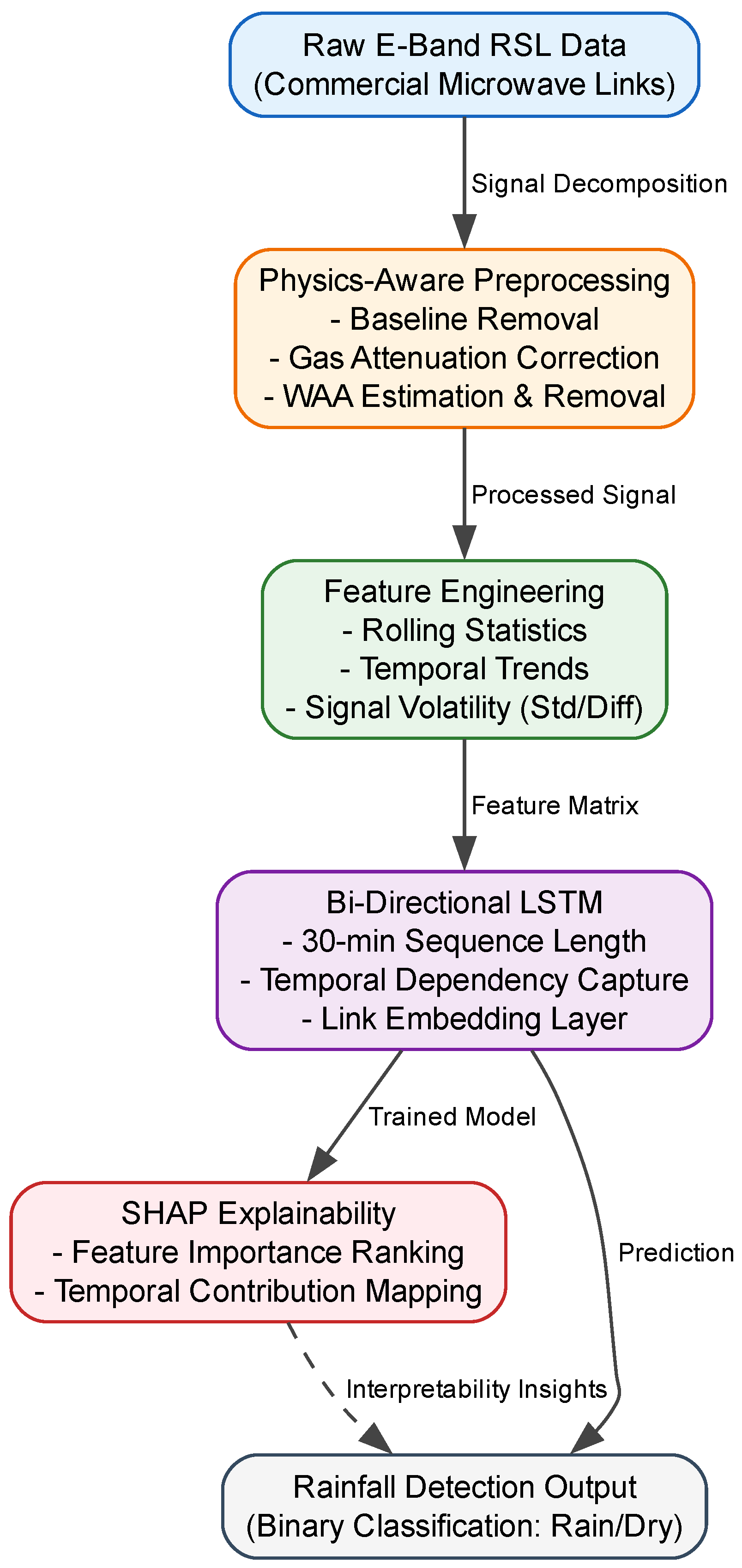
To illustrate the end-to-end processing pipeline, from raw signal inputs through physics-aware decomposition and feature engineering to the deep learning model and explainability outputs, Figure 1 outlines the general framework of the methodology.

To isolate the rain-induced signal from parasitic components, we adopt the decomposition framework described in the introduction. Within this framework, the communication signal is interpreted as an environmental observable, enabling its use as part of a distributed microwave sensing system. The total loss $L_t$ is expressed as (Equation (1)):

$$L_t=B+A_{gas}+A_{rain}+A_{WAA}+\epsilon$$

(1)

The baseline B is calculated using a one-week centered moving median filter, providing a stable reference that accounts for long-term hardware drift and antenna misalignment [5]. Gaseous attenuation $A_{gas}$ is incorporated using the Liebe MP model (1993), accounting for local atmospheric pressure, temperature, and humidity [5].

In practice, the rain-induced attenuation used in the machine learning pipeline (attenuation_rain) is computed as (Equation (2)):

$$A_{rain}=\max (0, L_t-B-A_{gas}-A_{WAA})$$

(2)

and subsequently clipped to non-negative values to ensure physical interpretability.

The most critical step in the physical modeling phase is the initial estimation of the wet antenna attenuation $A_{WAA}$ [7]. Based on the methodology proposed by Fencl et al. (2020) [5], the median attenuation during dry periods immediately following rainfall is used to estimate a constant WAA offset for each link. This serves as a baseline for the subsequent data-driven classification of WAA states.

3.3. Advanced WAA Detection and Signal Dynamics

Traditional WAA correction often fails because it does not account for the temporal evolution of the drying radome [7]. In this work, we employ an “Advanced WAA Detection” strategy based on physically interpretable signal dynamics. We define the “drying phase” as the period where the antenna radome is wet but active rainfall has ceased.

A time step is classified as WAA if it meets the following physical criteria:

• Ground truth rainfall intensity is zero.
• Rainfall was detected in the previous 1–3 min.
• The signal shows a monotonically decreasing trend (drying).
• The rolling standard deviation of the signal is below a specific threshold (smooth dynamics) [7].

It should be emphasized that ground-truth rainfall information is used exclusively during preprocessing for labeling and analysis purposes. The trained model does not rely on ground-truth inputs during inference and operates solely on signal-derived features. This approach allows the model to distinguish between stochastic, high-volatility attenuation caused by raindrops and the smooth, deterministic relaxation of the drying radome surface.

3.4. Feature Engineering for Temporal Sensing

To enable the deep learning model to act as a physical signal interpreter, we construct a feature vector that encodes both the instantaneous state and the temporal context of the link. This approach follows established methodologies in dynamic feature engineering aimed at mitigating signal instabilities and concept drift in industrial sensor data [28].

These features are calculated on a sliding window basis, providing the Bi-LSTM model with a temporal “image” of the signal’s behavior over the preceding 30 min.

3.5. Bi-LSTM Model Architecture and Training

The core of the sensing framework is a bi-directional LSTM network [22]. Unlike standard LSTMs, the Bi-LSTM processes the sequence in both forward and backward directions, allowing the model to utilize information from both the “past” and the “future” context for any given time step.

The architecture consists of:

• Input Layer: 30 min sequence of the features defined in

  Table 2. Physics-Aware Features Used for Rainfall Detection.

  Feature Name	Description	Physical Motivation
  attenuation_rain	Estimated rain-induced attenuation	Direct measure of path-integrated liquid water [5]
  loss_diff	1st-order temporal difference	Captures rapid onset and cessation of rain [22]
  loss_rolling_std	Rolling standard deviation (15 min)	Quantifies signal volatility associated with scattering (this study)
  loss_trend	Rolling mean trend (15 min)	Distinguishes between drying (WAA) and rain intensity shifts (this study)
  increase_streak	Persistence of signal increase	Identifies cumulative growth of rain events (this study)
  diff_pos/diff_neg	Positive/negative temporal dynamics	Separates wetting and drying rates (this study)
  range_15	Max–min amplitude range	Captures peak intensity fluctuations [2]
  hour	Time-of-day information	Accounts for diurnal baseline and humidity variations (this study)

  .
• Embedding Layer: A learned embedding representation associated with each link identifier is used to capture global hardware-related characteristics. Although embeddings are defined for all links, no temporal samples from validation links are used during training. As a result, embeddings associated with unseen links act as weak priors and do not introduce information leakage.
• LSTM Layers: Two bidirectional layers with 128 hidden units each, enabling modeling of long-term dependencies and temporal patterns [20].
• Dense Layers: A fully connected head with dropout (0.4) to prevent overfitting.
• Output Layer: Sigmoid activation providing the probability of rainfall.

Training was performed using binary cross-entropy loss and the Adam optimizer. The classification threshold was determined by maximizing the F1-score on the validation set via grid search. To address class imbalance, a positive class weight (pos_weight $=12.0$) was applied within the BCEWithLogitsLoss function. To improve robustness, Gaussian noise augmentation (NOISE_LEVEL $=0.15$) was injected into the input sequences during training.

3.6. Cross-Link Evaluation and Generalization

A critical requirement for practical deployment is the ability of a model to generalize to previously unseen conditions without re-training [29]. To ensure rigorous generalization, avoid bias associated with link-specific deployment conditions, and address transferability, we implemented a time-block shuffling validation strategy.

The complete dataset encompassing all 12 links (1a–6b) was sorted chronologically and partitioned into 10 distinct continuous temporal blocks. From these, 7 blocks were assigned for training, while the remaining 3 blocks served as an independent validation set. This approach guarantees temporal independence while ensuring that both subsets reflect the full heterogeneity of link lengths (0.39–4.87 km), signal-to-noise ratios, and meteorological conditions.

This experimental design prevents information leakage and enables a rigorous assessment of general transferability across heterogeneous network configurations rather than merely extrapolating to shorter/lower-SNR links. While this approach does not explicitly isolate strict cross-link transfer, it enables evaluation across heterogeneous link configurations and SNR regimes in a statistically consistent manner.

3.7. Baseline Methods and Benchmarking

Four baseline methods provide a point of comparison:

• Static Threshold: Rainfall is detected if $A_{rain}>2$ dB.
• k–R Model: The physical inversion using ITU-R P.838 parameters ($A=0.89·R^{1.12}$ for 73 GHz sublinks and $A=1.15·R^{1.06}$ for 83 GHz sublinks) [2].
• Logistic Regression: A linear classifier using the same feature set.
• Unidirectional LSTM (Uni-LSTM): A temporal baseline used to isolate the contribution of bidirectional processing.

3.8. Interpretability Analysis with SHAP

To understand the internal logic of the Bi-LSTM model, we apply SHapley Additive exPlanations [8]. The utility of SHAP in validating the architectural superiority and transparency of 1D deep learning models for signal-based diagnostics has been previously demonstrated in complex engineering tasks [30]. SHAP decomposes each prediction into contributions of individual features based on game-theoretic principles [31]. Global feature importance analysis is used to identify dominant predictors, while local dependence analysis provides insight into model response to specific signal dynamics.

3.9. Reproducibility

To ensure full transparency and reproducibility, the complete analytical pipeline, covering preprocessing, feature engineering, model training, and explainability, is provided in the Supplementary Materials (Listings S1–S6).

The source data are publicly available via the Zenodo repository, as stated in the Data Availability section. The hardware configuration (NVIDIA Quadro RTX 6000 GPU, see Appendix A) and computational environment (Python 3.12.3, PyTorch 2.12.0; Appendix B,

Table A1. Versions of Python libraries used in the computational environment.

Package	Description	Version
Core Scientific Stack
numpy	Numerical computations and array operations	v2.4.4
pandas	Data manipulation and tabular processing	v3.0.3
matplotlib	Generation of scientific visualizations and performance curves	v3.10.9
seaborn	Statistical data visualization	v0.13.2
Machine Learning & AI
torch	Deep learning framework (with CUDA 13.0 support)	v2.12.0+cu130
scikit-learn	Evaluation metrics, scalers, and baseline models	v1.8.0
shap	Explainable AI using SHapley Additive exPlanations	v0.51.0
joblib	Serialization of trained models and preprocessing pipelines	v1.5.3
Data I/O
pyarrow	Backend for high-performance Parquet data storage	v24.0.0
fastparquet	Alternative engine for Parquet file manipulation	v2026.3.0

) are fully documented.

All experiments were conducted with fixed random seeds and deterministic GPU settings (cuDNN) to minimize stochastic variability. As a result, the reported metrics are reproducible, with only minor numerical variation expected due to low-level system differences.

4. Results

4.1. Performance Comparison Across Validation Sets

The quantitative performance of the Bi-LSTM model compared to baseline methods is summarized in

Table 3. Comparative Performance Metrics Across All Links.

Link ID	Length (km)	F1 Static	F1 k–R	F1 Logistic Regression	F1 Uni-LSTM	F1 Bi-LSTM	Precision	Recall
1a	4.87	0.5532	0.6972	0.2713	0.6486	0.7744	0.6800	0.8991
1b	4.87	0.3826	0.6890	0.2188	0.5919	0.7700	0.6748	0.8965
2a	1.41	0.4921	0.5648	0.3796	0.7251	0.8081	0.7358	0.8961
2b	1.41	0.4877	0.5531	0.4692	0.7180	0.8101	0.7376	0.8982
3a	0.91	0.3050	0.3905	0.2535	0.5142	0.7112	0.6283	0.8192
3b	0.91	0.3021	0.3296	0.2804	0.4970	0.7196	0.6717	0.7750
4a	0.82	0.5059	0.5151	0.4492	0.5789	0.6901	0.5879	0.8353
4b	0.82	0.4835	0.5211	0.4380	0.6454	0.7256	0.6360	0.8446
5a	0.57	0.4890	0.5018	0.4591	0.7305	0.7422	0.6326	0.8978
5b	0.57	0.4943	0.5103	0.5103	0.7089	0.7562	0.6485	0.9069
6a	0.39	0.1857	0.2001	0.2529	0.7295	0.7555	0.6513	0.8993
6b	0.39	0.1793	0.1997	0.2186	0.7220	0.7520	0.6525	0.8873

for all evaluated links (1a–6b). The evaluation focuses on the F1-score, which provides a balanced measure of precision and recall. The physics-aware feature set used in the analysis is described in Table 2.

As shown in Table 3, the Bi-LSTM model consistently outperforms both the static threshold and the physical k–R models, achieving F1-scores above 0.74 even in challenging short-link regimes. The improvement is particularly pronounced in recall (exceeding 0.88), indicating an enhanced ability to detect low-intensity rainfall events that are often missed by traditional methods.

Importantly, the Uni-LSTM baseline, while substantially improving over non-sequential methods, consistently achieves lower F1-scores compared to the Bi-LSTM model. This confirms that bidirectional temporal context provides a measurable advantage in distinguishing rainfall from wet antenna attenuation, particularly under low signal-to-noise ratio conditions.

This behavior highlights the capability of sequence-based deep learning to extract meaningful temporal patterns. While classical methods struggle on shorter paths (such as 6a and 6b) due to limited path-integrated attenuation, where rain signals mix with instrumental noise and WAA [5,18], the Bi-LSTM model leverages temporal context over sliding windows and link-specific embedding layers to reliably differentiate rain from dry periods across heterogeneous link configurations.

It should be emphasized that the analysis encompasses independent temporal validation blocks representing challenging low-SNR regimes, particularly on shorter paths. Despite this, the model maintains robust discriminative performance across link lengths ranging from 0.39 to 4.87 km.

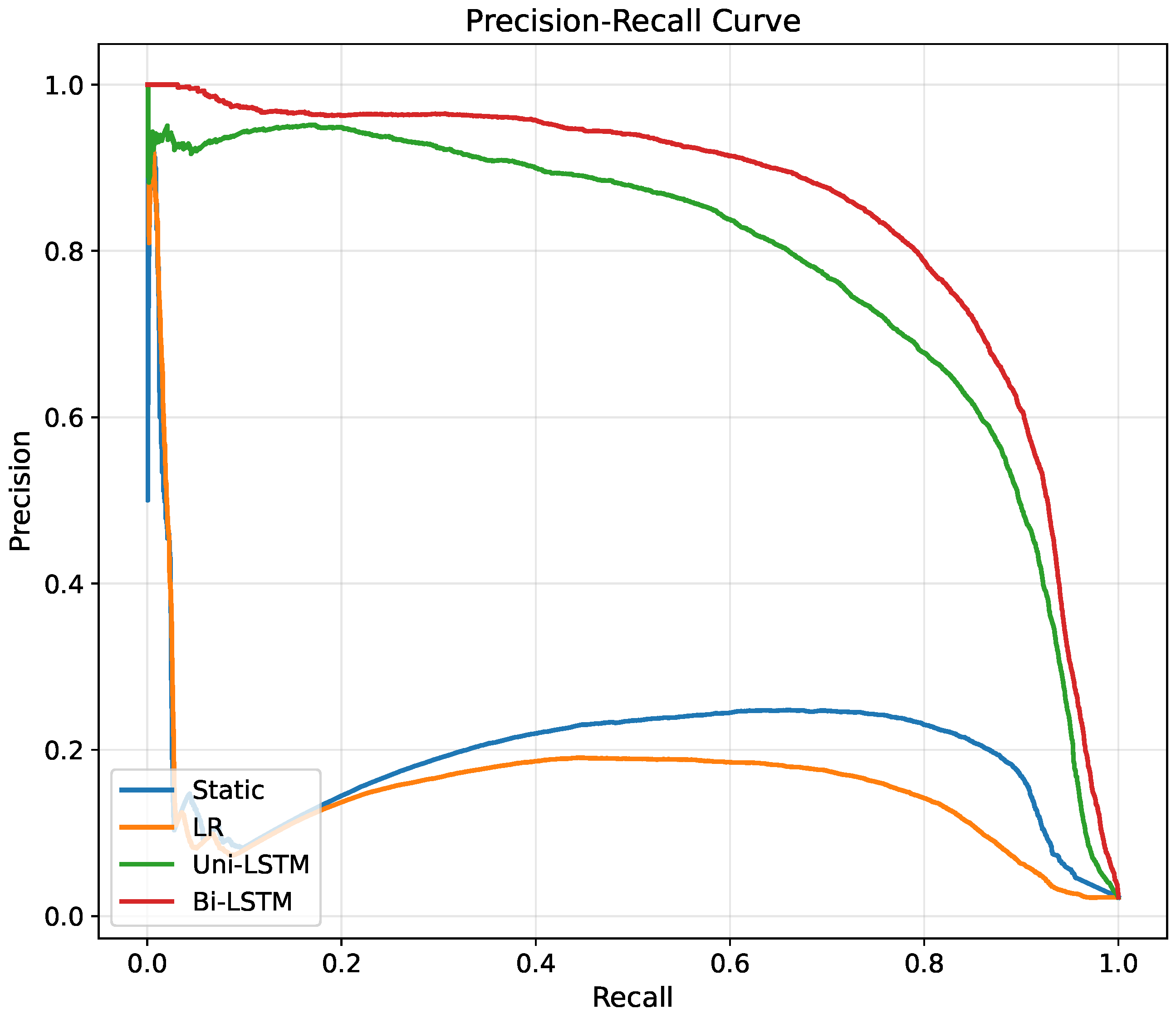
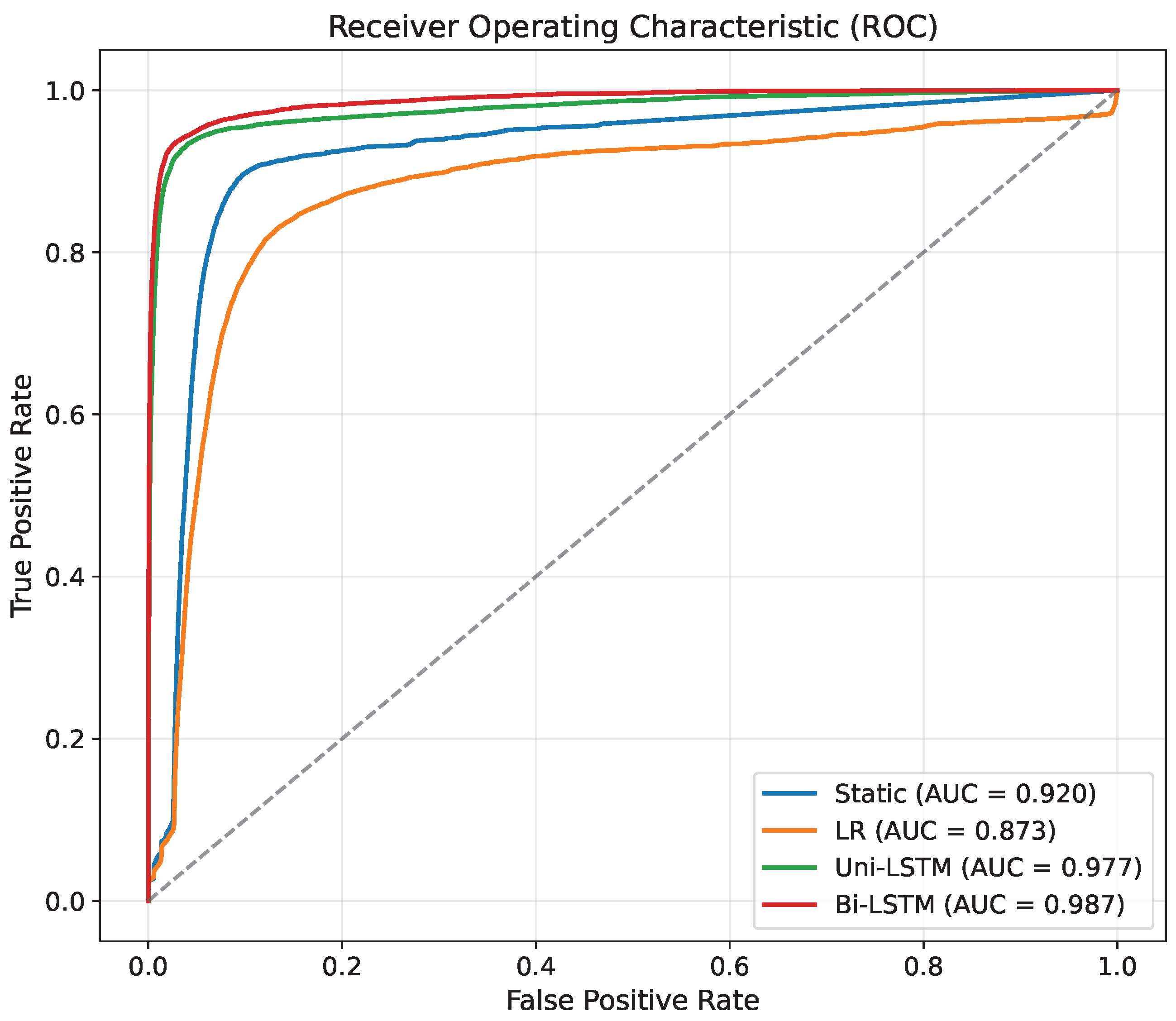
The performance trends observed in Table 3 are consistent with the ranking behavior shown in the Precision–Recall and ROC curves presented in Figure 2 and Figure 3.

As shown in Figure 2 and Figure 3, the Bi-LSTM model achieves strong performance in both Precision–Recall and ROC spaces, indicating a favorable trade-off between sensitivity and specificity across varying rainfall intensities. It should be noted that the classification threshold for the Bi-LSTM model was optimized to maximize the F1-score on validation data, whereas the ROC curve reflects threshold-independent ranking performance.

While the static baseline achieves competitive AUC values due to its direct physical interpretation, Logistic Regression generally underperforms compared to sequence-based approaches and is comparable to or below static baselines, reflecting its limited capacity to capture complex temporal dependencies. The Logistic Regression baseline achieves moderate performance, with F1-scores ranging from approximately 0.2 to 0.5, reflecting its ability to capture simple linear relationships in the data. In contrast, Uni-LSTM and Bi-LSTM significantly improve ranking performance, with gains exceeding 0.05–0.10 AUC compared to non-temporal baselines, and the Bi-LSTM achieving the highest AUC overall. This demonstrates that incorporating temporal context, particularly in a bidirectional manner, is critical for robust rainfall detection.

These results highlight a clear advantage of sequence-based models, where temporal modeling enhances both ranking capability and operational detection performance, especially in low-intensity rainfall regimes.

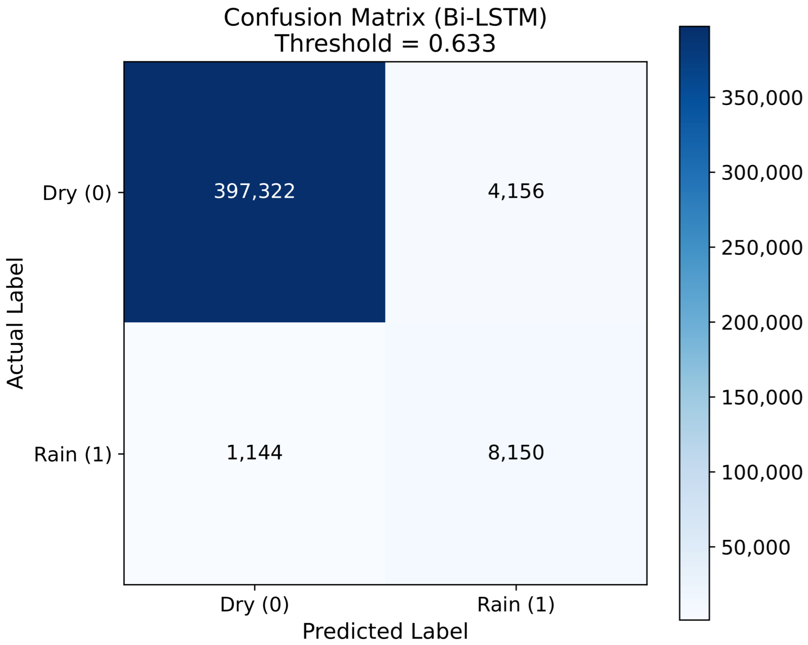
The confusion matrix in Figure 4 confirms that the model maintains a high true positive rate (recall) while effectively limiting false positives associated with wet antenna attenuation during the antenna drying phase. Analysis of shorter, noise-dominated links confirms that the Bi-LSTM successfully adapts its internal thresholds, keeping false alarm rates low and demonstrating resilience to instrumental uncertainty in low-SNR conditions across all link lengths. The confusion matrix reflects performance aggregated across all links and temporal validation blocks, including low-SNR short links where failure modes are most pronounced.

4.2. Rain Event Dynamics and Temporal Alignment

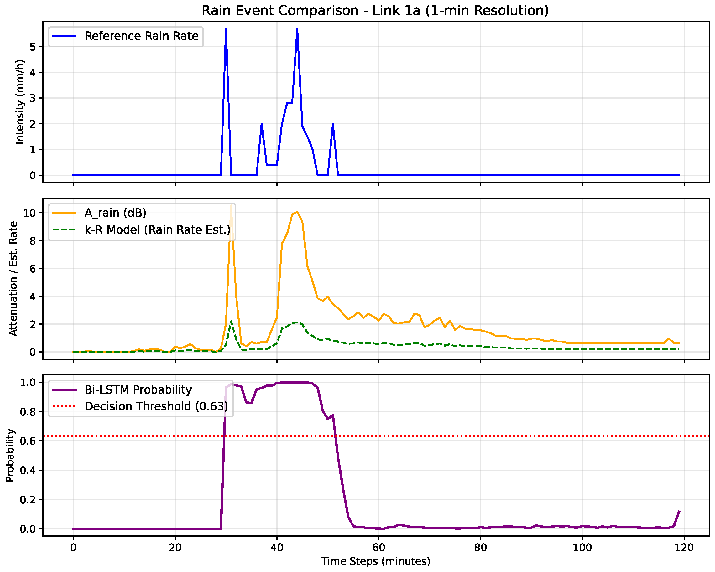
To demonstrate the performance of the proposed framework on a representative rainfall event at 1 min resolution, Figure 5 illustrates the time series of the reference rain rate, the physics-derived attenuation together with the classical k–R model estimation, and the output probability generated by the Bi-LSTM model alongside the calibrated decision threshold.

4.3. Feature Importance and Interpretability Analysis

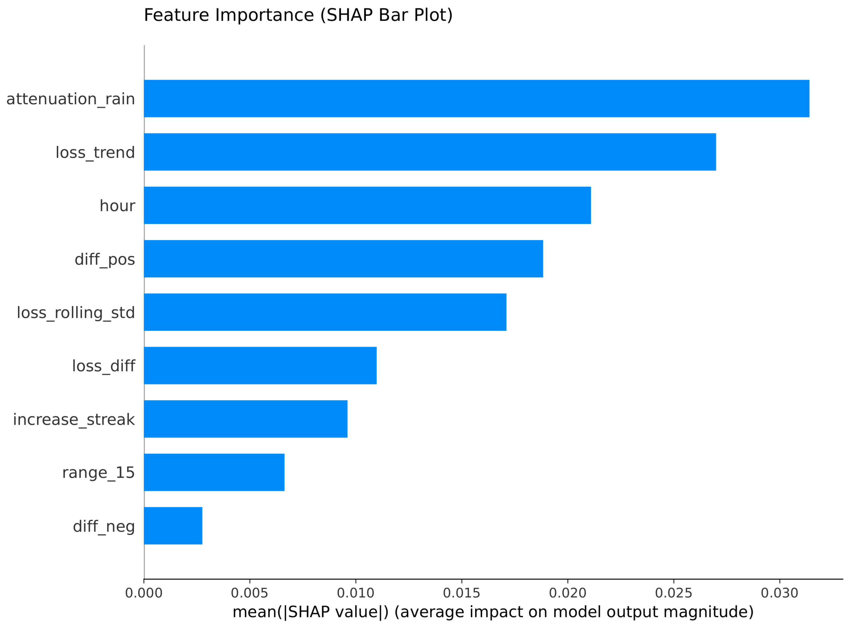
The SHAP analysis provides a clear ranking of the features that drive the model’s decisions. The global importance ranking is shown in Figure 6.

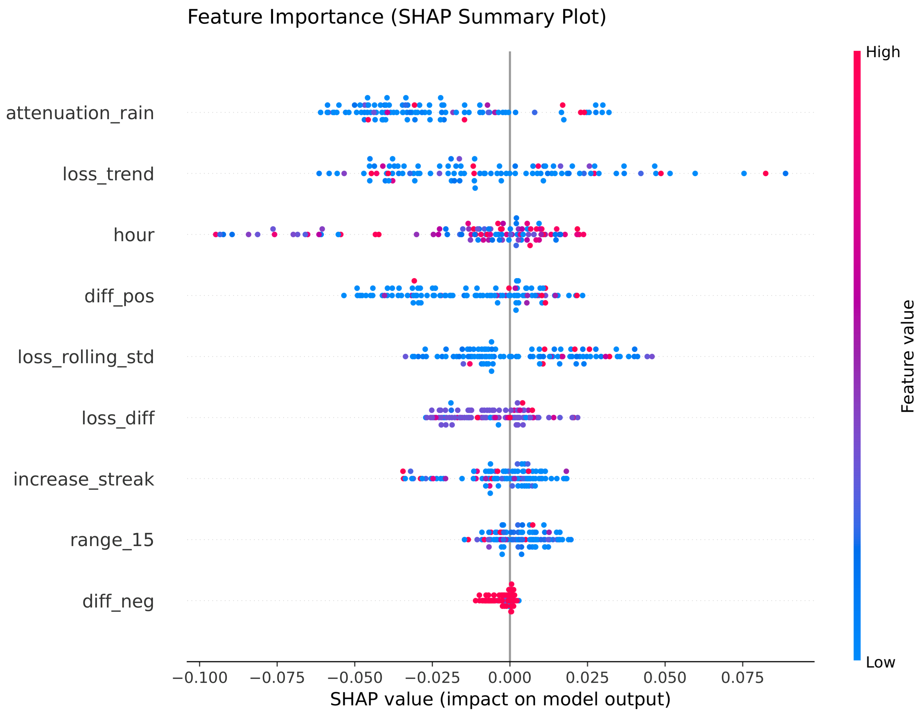
Features related to direct rain-induced attenuation (attenuation_rain) and temporal signal dynamics, specifically trend evolution (loss_trend) and signal volatility (loss_rolling_std), dominate the decision process. The distribution of SHAP values (Figure 7) confirms that the model has learned physically consistent relationships. High volatility and positive signal trends are associated with a higher probability of rain, while smooth, decreasing trends are correctly identified as no-rain (likely WAA) [7].

The beeswarm plot shows that high values of attenuation_rain, loss_trend, and increase_streak have a positive impact on the prediction (pushing the output toward “Rain”), consistent with the stochastic nature of precipitation.

4.4. Noise Robustness Stress Test

The robustness of the proposed microwave sensing framework was evaluated by injecting Gaussian noise directly into the raw attenuation signal across all links in the hold-out validation blocks. This setup reflects realistic instrumental uncertainty, where measurement noise primarily affects the received signal level. The results, summarizing the impact on classification performance across all evaluated links (1a–6b), are presented in

Table 4. Noise Robustness Test Results (F1-Score) across all links.

Link ID	Scenario	F1 Score	Performance Loss
1a	Clean	0.774	0.0%
	Noise (0.5 dB)	0.775	+0.1%
	Noise (1.0 dB)	0.772	−0.3%
1b	Clean	0.770	0.0%
	Noise (0.5 dB)	0.775	+0.6%
	Noise (1.0 dB)	0.761	−1.2%
2a	Clean	0.808	0.0%
	Noise (0.5 dB)	0.809	+0.1%
	Noise (1.0 dB)	0.802	−0.7%
2b	Clean	0.810	0.0%
	Noise (0.5 dB)	0.814	+0.5%
	Noise (1.0 dB)	0.807	−0.4%
3a	Clean	0.711	0.0%
	Noise (0.5 dB)	0.710	−0.1%
	Noise (1.0 dB)	0.703	−1.1%
3b	Clean	0.720	0.0%
	Noise (0.5 dB)	0.719	−0.1%
	Noise (1.0 dB)	0.721	+0.1%
4a	Clean	0.690	0.0%
	Noise (0.5 dB)	0.684	−0.9%
	Noise (1.0 dB)	0.676	−2.0%
4b	Clean	0.726	0.0%
	Noise (0.5 dB)	0.727	+0.1%
	Noise (1.0 dB)	0.729	+0.4%
5a	Clean	0.742	0.0%
	Noise (0.5 dB)	0.741	−0.1%
	Noise (1.0 dB)	0.729	−1.7%
5b	Clean	0.756	0.0%
	Noise (0.5 dB)	0.753	−0.4%
	Noise (1.0 dB)	0.747	−1.2%
6a	Clean	0.756	0.0%
	Noise (0.5 dB)	0.750	−0.8%
	Noise (1.0 dB)	0.735	−2.8%
6b	Clean	0.752	0.0%
	Noise (0.5 dB)	0.754	+0.3%
	Noise (1.0 dB)	0.755	+0.4%

.

It should be emphasized that the noise injection strategy differs from classical additive-noise sensitivity analyses. Rather than perturbing the entire feature space, noise was introduced exclusively at the level of the raw attenuation signal prior to feature engineering. As a result, derived features, such as rolling statistics, temporal trends, and persistence measures, retain their structure, enabling the model to leverage temporal context to mitigate high-frequency perturbations.

The results across all tested blocks indicate a high level of robustness. For both moderate-length and short links, the change in F1-score remains limited (generally within $\pm 3\%$), demonstrating that additive noise does not significantly degrade classification performance. The model retains predictive capability by relying on temporal consistency and embeddings [22].

For computational tractability, SHAP analysis was performed using a fixed link embedding, ensuring consistent interpretability while isolating the effect of temporal signal features.

4.5. Physical Separation of Rainfall and WAA Signatures

Finally, the physical distinction between rainfall and WAA was analyzed using the signal volatility metrics identified by SHAP.

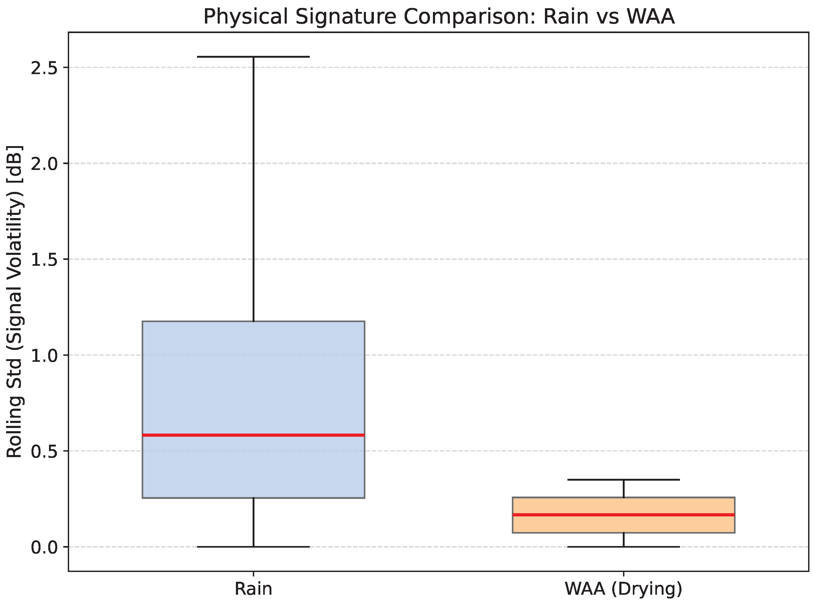
Rainfall events exhibit significantly higher variance and rolling standard deviation compared to antenna drying periods. The clear separation between these distributions validates the effectiveness of the advanced WAA detection strategy across all link lengths.

As shown in Figure 8, the “Advanced WAA” samples are characterized by very low volatility and monotonic decay, whereas “Rain” samples exhibit rapid fluctuations [7]. The Bi-LSTM model effectively exploits this separation to reduce false positives during the radome drying phase.

5. Discussion

5.1. Impact of Link Length on Microwave Sensing Performance

The most prominent result of this study is the strong dependence of sensing performance on link length in traditional methods [5]. While classical approaches exhibit significant performance degradation for shorter links (0.39–0.57 km; sublinks 5a–6b), where attenuation is limited, the proposed sequence-based deep learning framework achieves consistently high F1-scores across all evaluated links (Table 3), maintaining values above 0.74–0.75 even in low-SNR regimes. This behavior effectively mitigates the fundamental physical limitation imposed by short link lengths. While performance is significantly improved on short links, the results should be interpreted as relative improvements under the adopted temporal validation framework rather than complete elimination of physical sensing limits.

Although specific attenuation ($\mathrm{dB}/\mathrm{km}$) is high at these frequencies, the total path-integrated attenuation ($\mathrm{dB}$) for short links remains extremely limited. For example, a rainfall intensity of 5 mm/h results in less than 0.5 dB attenuation over a ∼400 m link, which is comparable to quantization noise (0.3–1.0 dB) and significantly smaller than typical wet antenna attenuation magnitudes (2–4 dB) [2].

By leveraging temporal context over sliding windows and link-specific embedding representations, the Bi-LSTM model extracts subtle and distributed signal dynamics. As a consequence, it successfully differentiates rain from non-rain states even in low signal-to-noise ratio regimes typical of short links, outperforming static thresholds and k–R models.

Importantly, this improvement is observed consistently across heterogeneous link lengths ranging from 0.39 to 4.87 km, indicating that the model learns transferable temporal patterns rather than link-specific characteristics.

From a system perspective, this finding demonstrates that advanced machine learning architectures can partially overcome the physical limitations of short backhaul links in environmental monitoring, enabling robust sensing across heterogeneous network topologies within ISAC-enabled environments [9].

5.2. Interpreting the Bi-LSTM: From Black Box to Physical Signal Processor

A recurring concern in applying deep learning to environmental sensing is the lack of interpretability [8]. However, the SHAP analysis demonstrates that the Bi-LSTM model relies predominantly on physically meaningful signal characteristics rather than spurious correlations.

The dominant contribution of direct rain-induced attenuation (attenuation_rain), signal volatility (loss_rolling_std), and temporal trends (loss_trend) indicates that the model exploits the fundamental distinction between stochastic and deterministic attenuation processes. Rainfall-induced attenuation exhibits high-frequency variability due to scattering on raindrops, whereas WAA corresponds to smoother temporal dynamics associated with antenna drying and water film evaporation [32].

These findings suggest that the Bi-LSTM operates as a temporal signal interpreter, extracting physically consistent patterns from attenuation time series rather than relying on static amplitude thresholds. This capability supports generalization across heterogeneous link conditions, as the model learns invariant temporal dynamics that are transferable across varying propagation regimes [29].

Importantly, the proposed framework does not rely solely on end-to-end data-driven learning. Instead, it integrates physics-based signal decomposition prior to model training, enabling the extraction of structured and physically consistent features. It should be emphasized that the term physics-aware refers to the incorporation of domain knowledge at the preprocessing and feature engineering stages, rather than embedding physical constraints directly within the model architecture or loss function.

5.3. WAA Modeling: Beyond Static Offsets

The separation between rainfall and WAA signatures (Figure 8) represents a significant improvement over traditional static offset approaches [7]. By incorporating temporal evolution, signal smoothness, and drying dynamics, the proposed framework provides a more physically consistent interpretation of attenuation signals.

Unlike rainfall-induced attenuation, which is inherently stochastic, WAA exhibits a quasi-deterministic decay behavior governed by antenna surface properties and environmental conditions. Explicit modeling of this behavior enables the proposed approach to reduce false positives during post-precipitation periods, which remain a major limitation in conventional CML-based rainfall detection methods.

5.4. Noise Robustness and Temporal Signal Filtering

The robustness analysis (Table 4) demonstrates that the proposed framework maintains stable performance under moderate noise perturbations applied directly to the attenuation signal.

Importantly, noise was introduced at the raw signal level (with an injection level of NOISE_LEVEL $=0.15$) prior to feature extraction, ensuring that derived temporal features retain their structural consistency. Under these conditions, the Bi-LSTM model exhibits high robustness, with performance variations not exceeding 2.8% even at 1.0 dB noise levels across all temporal validation blocks, including short links.

This behavior can be attributed to the intrinsic properties of sequence models, which aggregate information over time and can effectively filter local perturbations through temporal integration. In practical sensing scenarios, this suggests that moderate instrumental noise does not significantly degrade detection performance, provided that the underlying temporal signal structure is preserved.

Additionally, it is important to note that a purely data-driven Bi-LSTM operating directly on raw attenuation signals would likely exhibit reduced performance in this scenario. In E-band systems, raw signals are strongly influenced by non-rain components such as wet antenna attenuation, baseline drift, and hardware-related noise.

Without prior physical decomposition, a data-driven model would be required to implicitly learn these effects, which is particularly challenging under low-SNR conditions typical of short links. This can lead to overfitting, misclassification of WAA as rainfall, and reduced generalization across heterogeneous link configurations.

The proposed hybrid approach therefore provides a structured signal representation, allowing the Bi-LSTM to focus on physically meaningful temporal dynamics rather than compensating for raw signal artifacts.

5.5. Limitations and Future Work

Despite the strong performance of the proposed framework, several limitations should be acknowledged. First, while temporal modeling extends detection capabilities for short paths, microwave sensing remains fundamentally constrained by link geometry and path-integrated attenuation limits under extremely low SNR conditions.

Second, while the proposed WAA detection strategy captures key physical behaviors, it may still be sensitive to environmental edge cases such as fog, dew formation, or rapid meteorological transitions.

Third, although the evaluation encompasses a heterogeneous network of 12 sublinks, the limited number of independent physical link deployments restricts comprehensive statistical significance analysis, which should be addressed in larger-scale multi-link campaigns.

Fourth, although the temporal cross-validation setup enforces generalization across independent time blocks, further validation across diverse climatic regions and network topologies is required to assess full spatial and geographic transferability.

Future research directions include:

• Continuous Retrieval: Extension from rainfall detection to quantitative precipitation estimation using regression models.
• Multimodal Fusion: Integration of additional sensing sources, such as co-located meteorological measurements [33].
• Hybrid Physics–ML Models: Incorporation of physical constraints (e.g., the k–R relationship derived from ITU recommendations) directly into model architectures.
• Scaling to ISAC and 6G Systems: Extension of the framework to higher-frequency bands and integrated communication–sensing infrastructures [6].

6. Conclusions

This study presented a physics-aware deep learning framework for rainfall detection using E-band commercial microwave links. By leveraging existing telecommunication infrastructure, the proposed approach demonstrates how high-frequency communication signals can be repurposed as environmental sensing observables [9].

The main contributions include (i) the integration of physically motivated signal decomposition, (ii) the development of an advanced wet antenna attenuation detection strategy based on temporal dynamics, and (iii) the application of an interpretable Bi-LSTM model. It should be emphasized that the physics-aware aspect of the framework is realized through signal decomposition and feature engineering, rather than embedding physical constraints directly within the model architecture.

Experimental results show that temporal modeling significantly outperforms classical threshold-based and physical k–R approaches across all evaluated temporal validation blocks covering 12 sublinks (1a–6b). By utilizing sliding-window features, addressing severe class imbalance via loss weighting (pos_weight $=12.0$), and incorporating link-specific embeddings, the Bi-LSTM model maintains reliable performance even on very short paths ($0.39$ km), effectively mitigating conventional path-integrated attenuation limitations.

The proposed approach demonstrates robustness to moderate noise perturbations (with performance loss generally below 3%) and provides interpretable predictions consistent with microwave propagation theory and ITU-R guidelines. SHAP-based analysis confirms that the model relies on physically meaningful features, supporting its interpretation as a temporal signal processing system rather than a black-box predictor.

Overall, this framework establishes a physically consistent and interpretable methodology for exploiting E-band communication links as distributed sensing components within future ISAC-enabled networks.

References

1. Špačková, A.; Fencl, M.; Bareš, V. Information-theoretic analysis of commercial microwave link and environmental variables in rainfall estimation. Atmos. Meas. Tech. 2025, 18, 7445–7463. [Google Scholar] [CrossRef]
2. Lian, B.; Wei, Z.; Sun, X.; Li, Z.; Zhao, J. A Review on Rainfall Measurement Based on Commercial Microwave Links in Wireless Cellular Networks. Sensors 2022, 22, 4395. [Google Scholar] [CrossRef] [PubMed]
3. Zhang, P.; Liu, X.; Pu, K. Precipitation Monitoring Using Commercial Microwave Links: Current Status, Challenges and Prospectives. Remote Sens. 2023, 15, 4821. [Google Scholar] [CrossRef]
4. Wilk-Jakubowski, J.L.; Kuchcinski, A.; Wilk-Jakubowski, G.K.; Palej, A.; Pawlik, L. Digital Technologies and Machine Learning in Environmental Hazard Monitoring: A Synthesis of Evidence for Floods, Air Pollution, Earthquakes, and Fires. Sensors 2026, 26, 893. [Google Scholar] [CrossRef] [PubMed]
5. Fencl, M.; Dohnal, M.; Valtr, P.; Grabner, M.; Bareš, V. Atmospheric observations with E-band microwave links—Challenges and opportunities. Atmos. Meas. Tech. 2020, 13, 6559–6578. [Google Scholar] [CrossRef]
6. Huang, S.; Li, J.; Cao, J.; Fu, S.; Jin, Y.; Zhang, S. Performance Analysis for Integrated Sensing and Communication Systems in Rainfall Scenarios. Atmosphere 2025, 16, 1249. [Google Scholar] [CrossRef]
7. Doshi, S.C.; De Michele, C.; Cazzaniga, G.; Nebuloni, R. A Framework for Minimizing the Impact of Wet Antenna Attenuation on Rainfall Estimates Provided by Commercial Microwave Links. IEEE J. Sel. Top. Appl. Earth Obs. Remote Sens. 2026, 19, 421–437. [Google Scholar] [CrossRef]
8. He, Z.; Yang, Y.; Fang, R.; Zhou, S.; Zhao, W.; Bai, Y.; Li, J.; Wang, B. Integration of shapley additive explanations with random forest model for quantitative precipitation estimation of mesoscale convective systems. Front. Environ. Sci. 2023, 10, 1057081. [Google Scholar] [CrossRef]
9. Ostrometzky, J.; Messer, H. Opportunistic Weather Sensing by Smart City Wireless Communication Networks. Sensors 2024, 24, 7901. [Google Scholar] [CrossRef] [PubMed]
10. Messer, H.; Zinevich, A.; Alpert, P. Environmental Monitoring by Wireless Communication Networks. Science 2006, 312, 713. [Google Scholar] [CrossRef] [PubMed]
11. Leijnse, H.; Uijlenhoet, R.; Stricker, J.N.M. Microwave link rainfall estimation: Effects of link length and frequency, temporal sampling, power resolution, and wet antenna attenuation. Adv. Water Resour. 2008, 31, 1481–1493. [Google Scholar] [CrossRef]
12. Overeem, A.; Leijnse, H.; Uijlenhoet, R. Country-wide rainfall maps from cellular communication networks. Proc. Natl. Acad. Sci. USA 2013, 110, 2741–2745. [Google Scholar] [CrossRef] [PubMed]
13. Overeem, A.; Leijnse, H.; Uijlenhoet, R. Retrieval algorithm for rainfall mapping from microwave links in a cellular communication network. Atmos. Meas. Tech. 2016, 9, 2425–2444. [Google Scholar] [CrossRef]
14. Graf, M.; Chwala, C.; Polz, J.; Kunstmann, H. Rainfall estimation from a German-wide commercial microwave link network: Optimized processing and validation for 1 year of data. Hydrol. Earth Syst. Sci. 2020, 24, 2931–2950. [Google Scholar] [CrossRef]
15. E-Band (71–86 GHz) Guide: MmWave For 5G Backhaul. Tejte Blog. 2025. Available online: https://tejte.com/blog/e-band-71-86ghz-mmwave-5g-backhaul-guide/ (accessed on 15 May 2026).
16. Al-Samman, A.M.; Mohamed, M.; Ai, Y.; Cheffena, M.; Azmi, M.H.; Rahman, T.A. Rain Attenuation Measurements and Analysis at 73 GHz E-Band Link in Tropical Region. IEEE Commun. Lett. 2020, 24, 1368–1372. [Google Scholar] [CrossRef]
17. Bubniak, M.; Musil, P. Quantification of a Wet Antenna Attenuation for a Measurement of Rainfall Intensity via the Metropolitan Network of Microwave Links in 10 GHz Band. In Proceedings II of the 28st Conference STUDENT EEICT 2022: Selected Papers; The Faculty of Electrical Engineering and Communication, Brno University of Technology: Brno, Czech Republic, 2022. [Google Scholar] [CrossRef]
18. Pastorek, J.; Fencl, M.; Rieckermann, J.; Bareš, V. Precipitation Estimates from Commercial Microwave Links: Practical Approaches to Wet-Antenna Correction. IEEE Trans. Geosci. Remote Sens. 2022, 60, 4104409. [Google Scholar] [CrossRef]
19. Schleiss, M.; Rieckermann, J.; Berne, A. Quantification and Modeling of Wet-Antenna Attenuation for Commercial Microwave Links. IEEE Geosci. Remote Sens. Lett. 2013, 10, 1195–1199. [Google Scholar] [CrossRef]
20. Pudashine, J.; Guyot, A.; Petitjean, F.; Pauwels, V.R.N.; Uijlenhoet, R.; Seed, A.; Prakash, M.; Walker, J.P. Deep Learning for an Improved Prediction of Rainfall Retrievals From Commercial Microwave Links. Water Resour. Res. 2020, 56, e2019WR026255. [Google Scholar] [CrossRef]
21. Jacoby, D.; Ostrometzky, J.; Messer, H. Short-Term Prediction of the Attenuation in a Commercial Microwave Link Using LSTM-based RNN. In Proceedings of the 2020 28th European Signal Processing Conference (EUSIPCO), Amsterdam, The Netherlands, 18–21 January 2021. [Google Scholar] [CrossRef]
22. Scognamiglio, G.; Rucci, A.; Vaccaro, A.; Adirosi, E.; Sapienza, F.; Giannetti, F.; Bacci, G.; Angeloni, S.; Baldini, L.; Roversi, G.; et al. Deep Learning for Opportunistic Rain Estimation via Satellite Microwave Links. Sensors 2024, 24, 6944. [Google Scholar] [CrossRef] [PubMed]
23. Polz, J.; Chwala, C.; Graf, M.; Kunstmann, H. Rain event detection in commercial microwave link attenuation data using convolutional neural networks. Atmos. Meas. Tech. 2020, 13, 3835–3853. [Google Scholar] [CrossRef]
24. Nikraftar, Z.; Parizi, E.; Saber, M.; Boueshagh, M.; Tavakoli, M.; Esmaeili Mahmoudabadi, A.; Ekradi, M.H.; Mbuvha, R.; Hosseini, S.M. An Interpretable Machine Learning Framework for Unraveling the Dynamics of Surface Soil Moisture Drivers. Remote Sens. 2025, 17, 2505. [Google Scholar] [CrossRef]
25. Geng, H.; Wang, W.; Liu, J.; Benson, D. Landslide susceptibility modeling based on SHAP interpretability and ensemble learning: A case study in Fuyuan County, Southwest China. Front. Earth Sci. 2025, 13, 1731872. [Google Scholar] [CrossRef]
26. Palhares, V.; Grudnitsky, A.; Mandelli, S. Weather Estimation for Integrated Sensing and Communication. arXiv 2026, arXiv:2601.15145. [Google Scholar] [CrossRef]
27. Fencl, M.; Dohnal, M.; Mudroch, M.; Bareš, V. Data and Code for the Paper Atmospheric Observations with E-band Microwave Links–Challenges and Opportunities. Dataset. Zenodo, 2020. Available online: https://zenodo.org/records/4090953 (accessed on 15 May 2026). [CrossRef]
28. Pawlik, Ł. Mitigating Concept Drift in Wind Turbine Prognostics Using Dynamic Feature Engineering and Chronological Validation. IEEE Access 2026, 14, 44491–44502. [Google Scholar] [CrossRef]
29. Blettner, N.; Fencl, M.; Bareš, V.; Kunstmann, H.; Chwala, C. Transboundary Rainfall Estimation Using Commercial Microwave Links. Earth Space Sci. 2023, 10, e2023EA002869. [Google Scholar] [CrossRef]
30. Poliak, M.; Pawlik, L.; Frej, D. Explainable Deep Learning for Bearing Fault Diagnosis: Architectural Superiority of ResNet-1D Validated by SHAP. Electronics 2025, 14, 4875. [Google Scholar] [CrossRef]
31. Sen, D. Explainable Deep Learning for Time Series Analysis: Integrating SHAP and LIME in LSTM-Based Models. J. Inf. Syst. Eng. Manag. 2025, 10, 412–423. [Google Scholar] [CrossRef]
32. Tiede, J.; Chwala, C.; Herpers, C.; Paulus, A.H.; Siart, U.; Eibert, T.F. Electromagnetic Water Drop Model for Wet Antenna Attenuation Based on Near-Field Measurements. IEEE Trans. Antennas Propag. 2025, 73, 9355–9364. [Google Scholar] [CrossRef]
33. Wang, Y.; Jiang, H.; Liu, G.; Chen, Q.; Ni, M. Research on Real-Time Rainfall Intensity Monitoring Methods Based on Deep Learning and Audio Signals in the Semi-Arid Region of Northwest China. Atmosphere 2026, 17, 131. [Google Scholar] [CrossRef]
Figure 1. System architecture and processing pipeline for rainfall detection using E-band CML data.
Photonics 13 00595 g001
Figure 2. Precision–Recall curve comparing static, Logistic Regression, Uni-LSTM, and Bi-LSTM models.
Photonics 13 00595 g002
Figure 3. Receiver Operating Characteristic (ROC) curves comparing static, Logistic Regression, Uni-LSTM, and Bi-LSTM models evaluated on independent temporal validation blocks.
Photonics 13 00595 g003
Figure 4. Confusion matrix for the Bi-LSTM model evaluated on validation data subsets.
Photonics 13 00595 g004
Figure 5. Exemplary rainfall event comparison for Link 1a, showing reference rain rate, rain-induced attenuation with kR model estimates, and the Bi-LSTM detection probability.
Photonics 13 00595 g005
Figure 6. Global Feature Importance Ranking (SHAP).
Photonics 13 00595 g006
Figure 7. SHAP Value Distribution Across Features.
Photonics 13 00595 g007
Figure 8. Signal Volatility Comparison: Rain vs Wet Antenna Attenuation.
Photonics 13 00595 g008