Article

Form Error Compensation for Freeform Mirrors Made of Aluminum Silicon Alloy in Ultra-Precision Diamond Turning

1
School of Mechanical Science and Engineering, Huazhong University of Science and Technology, Wuhan 430074, China
2
Huazhong Institute of Electro-Optics, Wuhan 430223, China
3
School of Mechanical Engineering and Electronic Information, China University of Geosciences, Wuhan 430074, China
4
PGMF and School of Physics, Huazhong University of Science and Technology, Wuhan 430074, China
*
Author to whom correspondence should be addressed.
Photonics 2026, 13(6), 580; https://doi.org/10.3390/photonics13060580
Submission received: 27 April 2026 / Revised: 1 June 2026 / Accepted: 9 June 2026 / Published: 14 June 2026
(This article belongs to the Special Issue Advances in Optical Precision Manufacturing and Processing)

Abstract

A complex curved reflector made from a 40% silicon–aluminum alloy (AlSi40) can meet the requirements of optical systems operating across the infrared, near-infrared, and visible bands. It enables an athermalization design with simplified alignment and assembly, while offering high manufacturing efficiency and low costs. This makes it ideal for widespread use in high-end optical systems. As an enabling technology for the fabrication of AlSi40 freeform mirrors, error compensation in ultra-precision (UP) diamond turning is currently a research hotspot; however, current error compensation methods still have considerable room for improvement in terms of both accuracy and manufacturing efficiency. To address this issue, this study proposes an efficient and highly accurate method: a polar grid is defined in the machining coordinate system, and the corresponding surface point cloud is calculated. Using measured point clouds from reference spheres and freeform form error in the measurement coordinate system, mounting pose errors and form error with measurement error removed are determined via least squares. Machining error at grid points is then calculated via coordinate transformations and bicubic spline interpolation, and applied to correct cutter contact points (CCPs). Cutter location points (CLPs) are finally obtained using piecewise cubic spline fitting and a bisection method. With this method, average form error of four AlSi40 substrates improved from RMS 114.8 nm to 47.9 nm, and for four AlSi40 substrates with nickel–phosphorus (NiP)-plated surfaces, from RMS 71.3 nm to 31.1 nm. The compensated accuracy meets near-infrared stellar tracker requirements without polishing, greatly enhancing freeform mirror manufacturing efficiency.

1. Introduction

Freeform surfaces can significantly improve the imaging quality and reduce the size and weight of optical systems [1,2,3]. Therefore, in the last 10 years, freeform optics has enabled compact and high-performance imaging systems and is expected to become the preferred design for advanced optical systems in the coming decades [4,5,6,7,8,9,10,11,12,13]. AlSi40 offers high elastic modulus (102 GPa), low density (2540 kg/m3), high thermal conductivity, and can be polished to sub-nanometer roughness after NiP plating. It can meet the requirements for optical systems operating in the infrared, near-infrared, visible, and even ultraviolet bands, enables athermalization design with simplified alignment and assembly, and features high manufacturing efficiency and low costs. Therefore, it has broad application prospects in high-end optical systems [14,15,16,17,18,19,20,21,22].
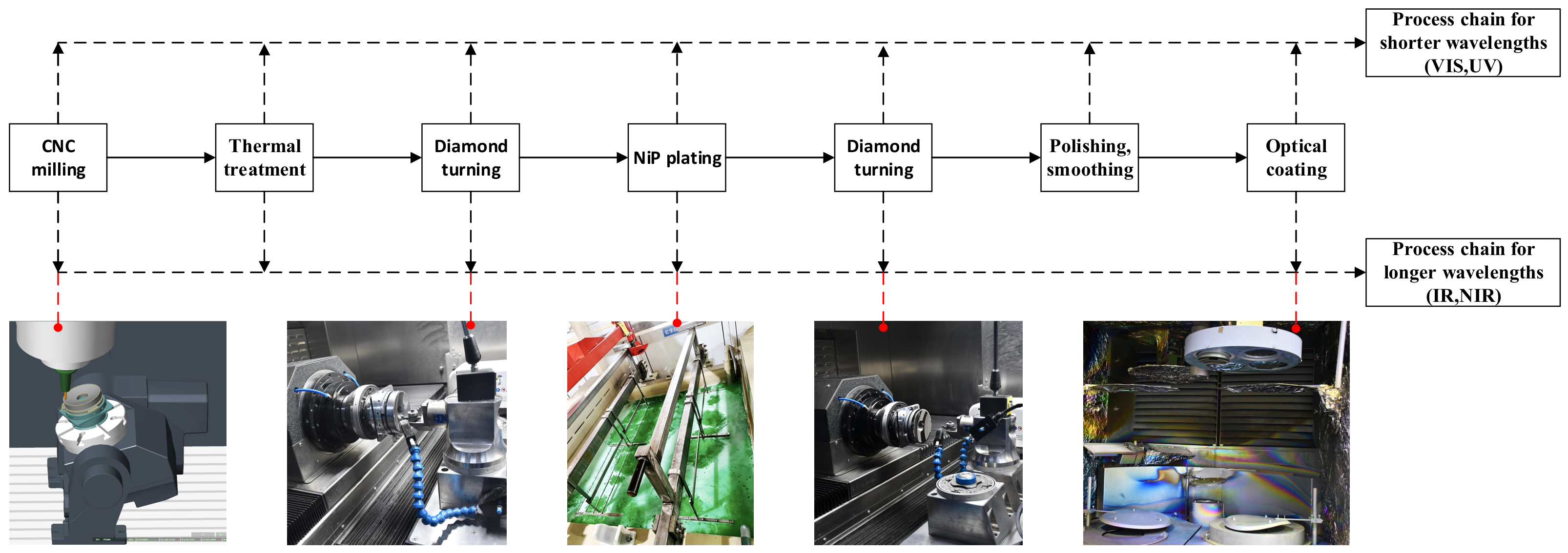
As shown in Figure 1, the main manufacturing process for AlSi40 mirrors comprises: milling, heat treatment, UP diamond turning of the substrate, NiP plating, UP diamond turning of the NiP-plated surface, polishing, and coating. The precision of UP diamond turning of the substrate affects the uniformity of the NiP-plated layer thickness and the stability of the mirror, while the UP diamond turning accuracy of the NiP-plated surface influences the manufacturing precision and efficiency of the optical surface of the mirror. Therefore, as an enabling technology for the fabrication of AlSi40 mirrors and freeform surfaces, error compensation in UP diamond turning is currently a research hotspot [7,23]. Regarding error compensation and tool path optimization in UP turning, numerous scholars have systematically conducted the following research.
In terms of error compensation: Nicholas W. Horvath et al. [24] proposed correcting tool mounting errors and tool radius errors by turning a spherical surface prior to the turning of freeform mirrors; however, they did not provide any theoretical or experimental results. LEE W. B. et al. [25] investigated a method for compensating residual form errors of workpieces through tool offset in UP turning of aspherical surfaces; this method involves altering only the tool center coordinates and essentially compensates for systematic tool setting errors, and is applicable only to aspherical surfaces. Kodai Nagayama K. et al. [26] calculated tool mounting errors, tool radius errors and tracking errors by turning freeform surfaces, and compensated for these errors using a feedforward method. In actual machining, these errors interact to affect the surface profile of the workpiece, and it is difficult to completely decouple them through a single test cut. Furthermore, this method cannot compensate for out-of-model errors, such as machine tool geometric errors. R.A. Parker et al. [27] proposed a method for compensating tool setting errors and tool wear based on interferometry. Peng et al. [28] proposed a method for calculating tool setting errors and tool radius errors in UP turning based on the least squares method. Nagayama K. et al. [29] proposed a method to compensate for tool waviness by directly measuring it using a white light interferometer. Ruibin Liang et al. [30] proposed a test-cutting method, which involves measuring the test-cut spherical workpiece using a white-light interferometer to calculate the tool waviness error and thereby apply compensation. Zhang et al. [31] developed a neural network-based method for compensating for servo errors in UP turning. Takeshi Hashimoto et al. [32] investigated the compensation of time delay errors in the c-axis of a fast tool servo under high rotational speeds. Similarly, the aforementioned methods cannot compensate for out-of-model errors. Furthermore, regarding the measurement and compensation of tool waviness errors, previous studies have not adequately accounted for the pose errors matching between the tool and workpiece in the measurement coordinate system and the machining coordinate system. Laura Hopper et al. [33] proposed a method for measuring and compensating the geometric errors of a four-axis UP lathe using a confocal sensor. He et al. [34] compensated for geometric and tracking errors in the machine tool by turning freeform surfaces, mapping these errors to the tool path for correction. Chen et al. [35,36] introduced a method for measuring rotationally symmetric higher-order freeform surfaces using CGH and compensating the machining error by mapping them onto the tool path. WANG et al. [37] introduced an on-machine measurement method for compensating form errors by fitting them using Zernike polynomials. Yu et al. [38] proposed an iterative compensation method for machining error of freeform surfaces using CGH measurement. The aforementioned research relies primarily on a strategy that maps surface shape errors onto tool paths for multiple iterative corrections. As this method does not account for tool compensation, it introduces inherent computational errors, and the multiple iterations limit improvements in compensation efficiency; furthermore, the use of the computer-generated holography (CGH) measurement method suffers from limitations, including long production cycles and low measurement efficiency.
In terms of tool path optimization (including calculation of CCP and CLP): Zhu Z et al. [39] proposed a novel adaptive tool servo (ATS) diamond turning technique, the primary objective of which is to improve machining efficiency rather than to compensate for machining error. He S et al. [40] proposed a new spiral tool path generation method based on a nonuniform rational B-spline (NURBS) parameter space for the UP diamond turning of freeform surfaces. You K et al. [41] proposed a universal location-point-drive tool path generation method. Ao S et al. [42] proposed a smooth tool path interpolation algorithm in the non-cutting area for ultra-precision turning of discontinuous multi-freeform surfaces. Guo Y et al. [43] proposed a multi-objective optimization method for tool path generation based on a novel surface analysis model. The primary objective of the above methods is to optimize machining efficiency and minimize machining error, rather than to compensate for them. Marco Buhmann et al. [44] presented a method for generating tool paths by estimating normal vectors through fitting planes to neighboring point clouds. This method can be used for surface error compensation; however, as it relies on local plane fitting to calculate the normal vector rather than using an exact analytical solution, it introduces a fundamental computational error.
With regard to error compensation for complex machining objects, such as freeform surfaces, existing methods [24,25,26,27,28,29,30,31,32,33,34,35,36,37,38,39,40,41,42,43,44] still suffer from several significant issues: Firstly, regarding the measurement and compensation of tool waviness errors, previous studies have not adequately accounted for the pose errors matching between the tool and workpiece in the measurement coordinate system and the machining coordinate system. Secondly, existing research has already demonstrated the ability to effectively address typical sources of error, such as tool offset, tool radius errors and trajectory-following errors. However, during actual machining processes, the machining accuracy of surface profiles is also influenced by other error factors not incorporated into current models; existing methods are not yet capable of effectively compensating for such out-of-model errors; Thirdly, regarding surface form error (SFE) compensation, current approaches primarily rely on strategies that map SFE onto the tool path for iterative correction; this method contains a fundamental error and requires multiple iterations, thereby limiting improvements in compensation efficiency and accuracy. Fourthly, with regard to the measurement of SFE, computer-generated holography (CGH) suffers from limitations, including long production cycles and low measurement efficiency. Compared with the CGH method, using a profilometer to measure freeform surfaces offers the advantage of significantly higher efficiency. However, when mounting a freeform surface on the profilometer, the mounting pose errors of the surface in the measurement coordinate system cannot be accurately determined. To address the above issue and meet the demand for high-efficiency and high-precision manufacturing of an AlSi40 mirror for a near-infrared stellar tracker optical system, this study proposes a compensation method using form error measurement data obtained from a non-contact profilometer.

2. Materials and Methods

2.1. Parameters of the Stellar Tracker Optical System and Its Mirrors

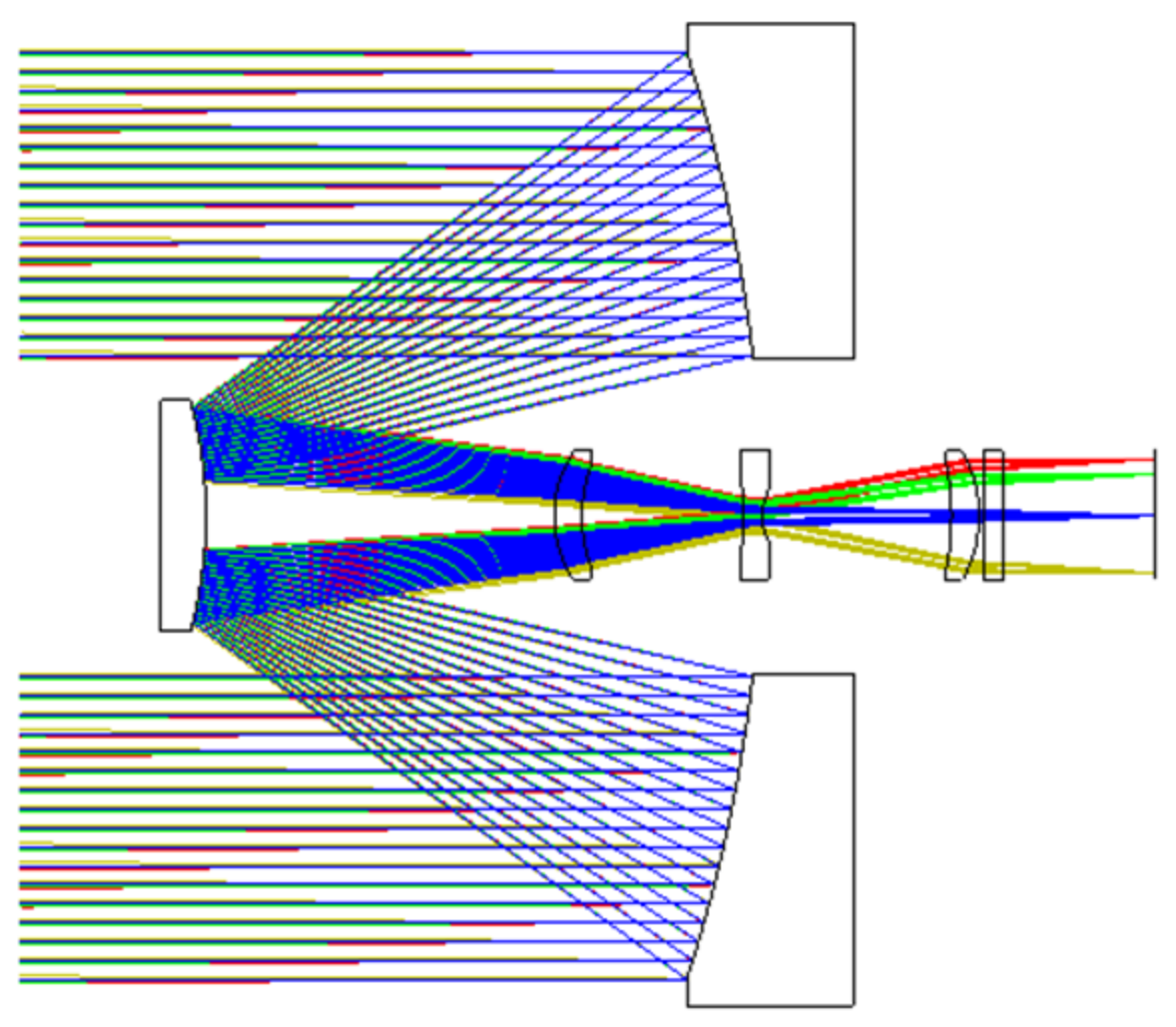
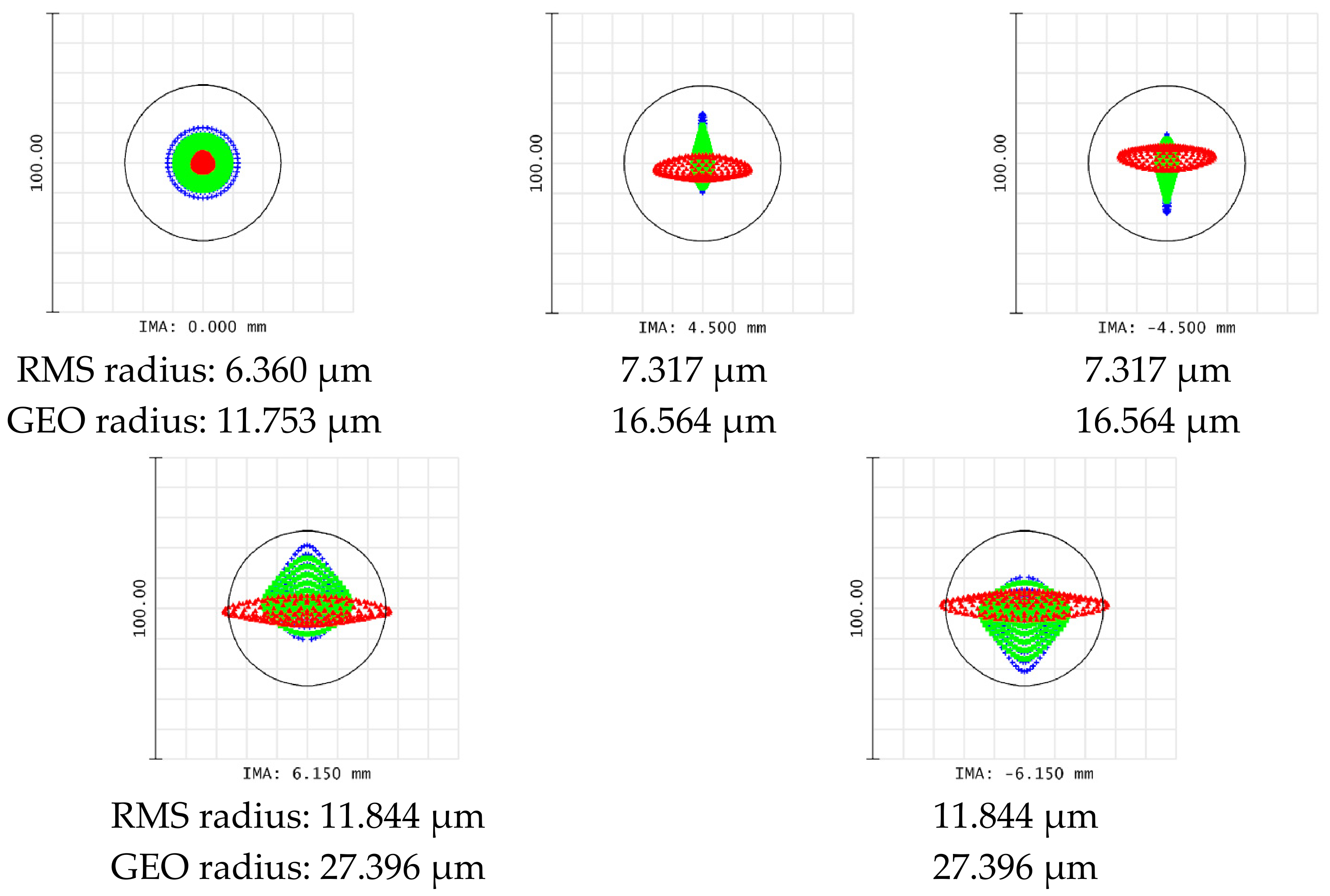
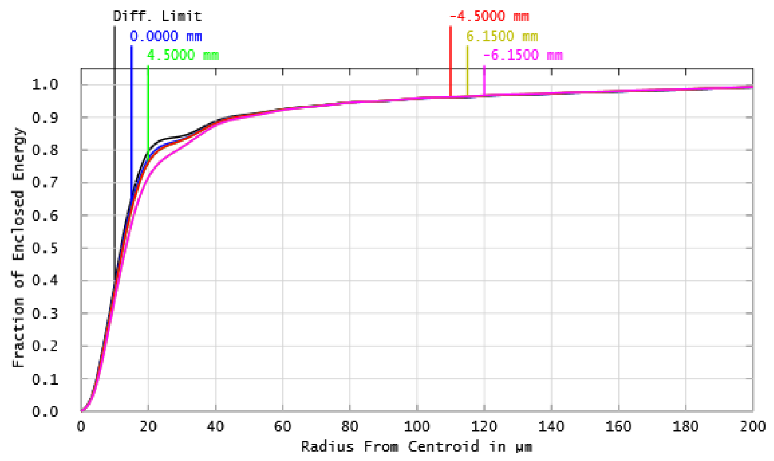
The design parameters and layout of the near-infrared stellar tracker optical system are shown in Table 1 and Figure 2, respectively. The operating wavelength range is 1360~1700 nm, with a focal length of 1500 mm and a pupil diameter of 98 mm; the pixel size and number of pixels are 30 μm × 30 μm and 320 × 256 respectively. Both the primary mirror (M1) and secondary mirror (M2) employ XY polynomial freeform surfaces, the surface equations for which are shown in Equation (1); the parameters of M1 and M2 are given in Table 2. The point spread function of the system is shown in Figure 3. The RMS diameter of the diffraction spot in each field of view is less than 20 μm, satisfying the diffraction limit requirement. The diameter of the diffraction spot containing 80% of the energy in each field of view is shown in Table 3, and the energy concentration is shown in Figure 4. Across the entire field of view, the diameter of the imaging spot containing more than 80% of the energy is less than 60 μm, concentrated within a 2 × 2-pixel number, indicating a very high degree of energy concentration.
z = ( x 2 + y 2 ) / R 0 1 + 1 ( k + 1 ) ( 1 / R 0 ) 2 ( x 2 + y 2 ) + m = 0 p n = 0 p C ( m , n ) x m y n
In the equation, z represents the surface sag, x and y are the corresponding lateral coordinates, R 0 is the radius of curvature at the vertex of the surface, k is the conic coefficient of the surface, C ( m , n ) is the coefficient of the XY polynomial, and m and n represent the powers of x and y, respectively.
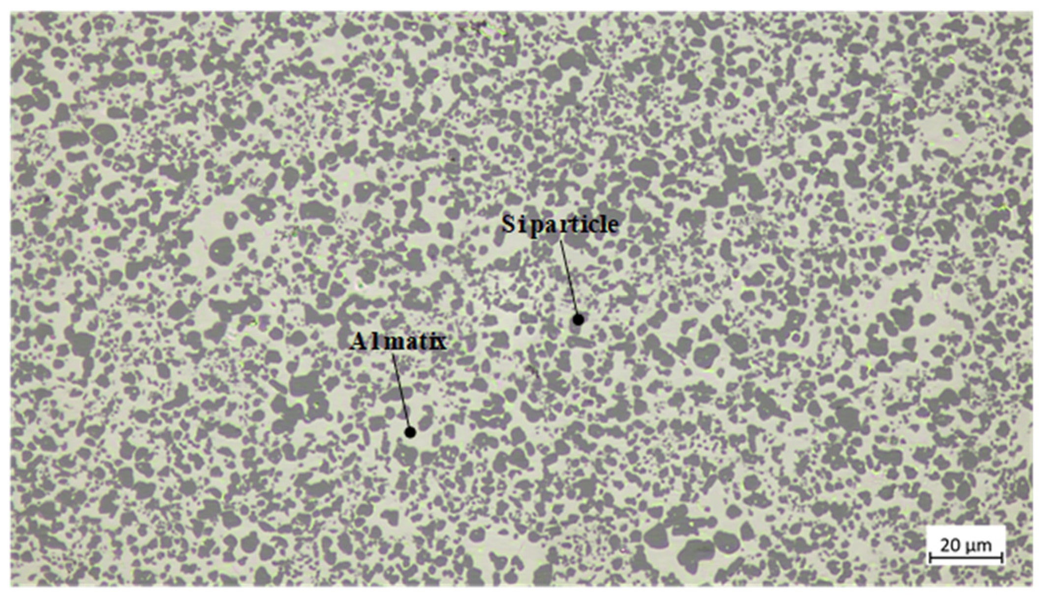
The metallographic image and technical parameters of the workpieces used in this study are shown in Figure 5 and Table 4, respectively. Workpiece No. 1 is made of AlSi40, while workpiece No. 2 is made of AlSi40 plated with NiP. The blanks were provided by the Institute of Metal Research (IMR), Chinese Academy of Sciences.

2.2. The Error Compensation Process and Methodology

To address the current inability of profilometers to accurately determine the mounting error of a freeform surface rotating about the z-axis in the measurement coordinate system, this study employs four reference spherical surfaces. Based on the least squares method, the mounting error of the freeform surface rotating about the z-axis of the measurement coordinate system is calculated using the measured point clouds of the reference spherical surfaces in the measurement coordinate system. The remaining mounting errors of the freeform surface on the profilometer are then calculated using the form error of the freeform surface. Subsequently, the measurement error induced by the mounting pose errors is removed to obtain the accurate SFE, which is then used for error compensation.
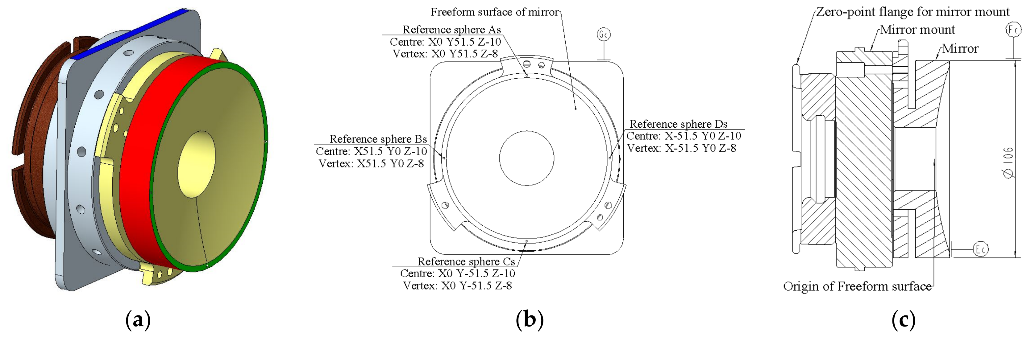
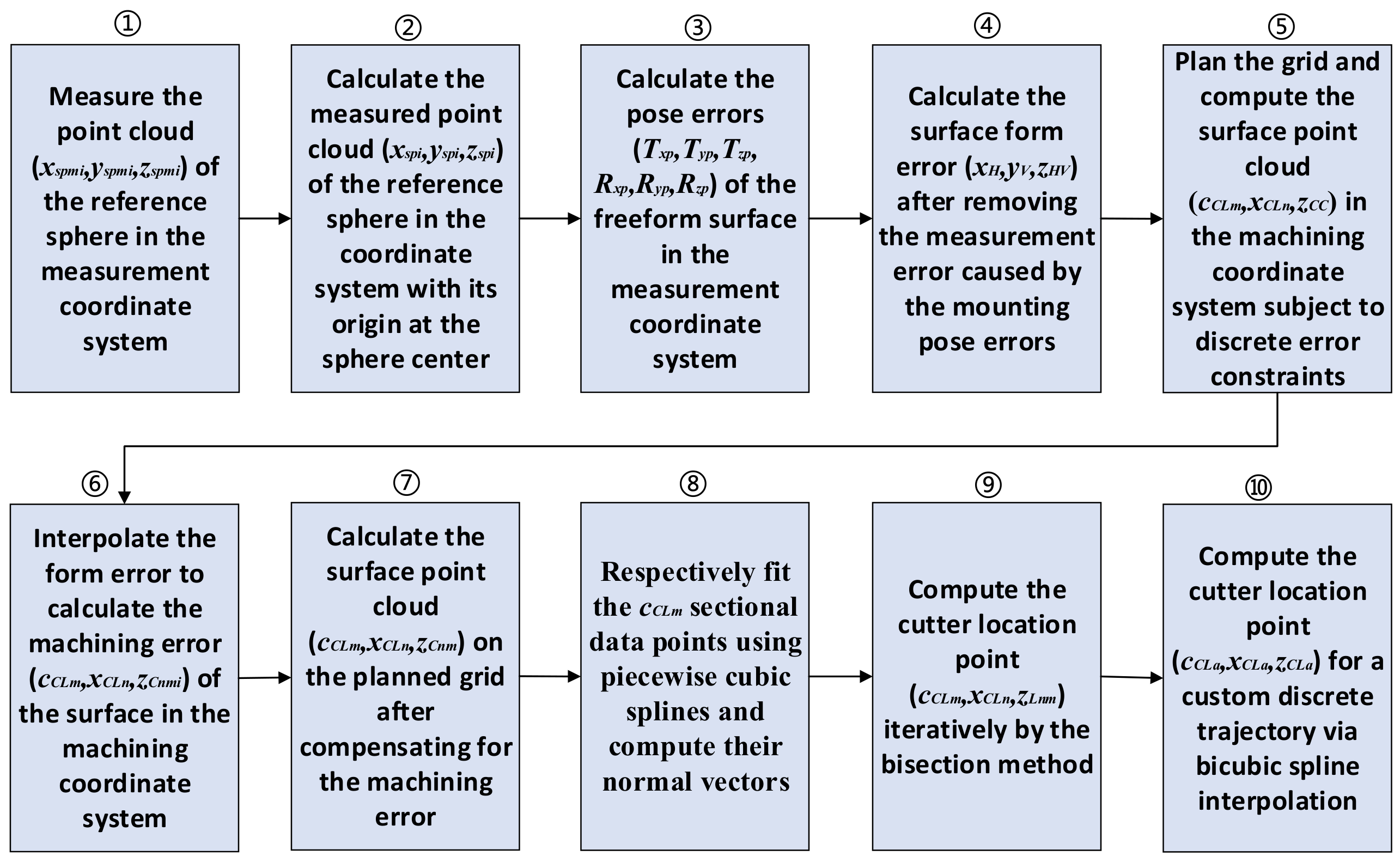
Taking M1 in this study as an example, the mirror is first mounted on a fixture, which is then connected to the flange of the zero-point positioning system; it is subsequently mounted via the flange onto the machine tool for machining or onto the profilometer for measurement. The reference features Ec, Fc and Gc, as well as the reference spheres As, Bs, Cs and Ds used to determine the position and orientation of M1, are shown in Figure 6. The end face Ec and outer cylindrical surface Fc were machined using the horizontal lathe (IL500), whilst the side face Gc was machined using the milling machine (Pyramid Nano). Subsequently, a machining coordinate system was established on the milling machine using the end face Ec, outer cylindrical surface Fc and side face Gc, and four reference spherical surfaces (As, Bs, Cs, Ds) were machined. The radius of curvature for all four reference spheres is 2 mm. The coordinates of the reference spheres are shown in Figure 6. The end face Ec, the outer circumference Fc and the four reference spheres (As, Bs, Cs, Ds) are used to help define the measurement coordinate system, thereby ensuring that surface milling, UP turning and measurement share a common datum. The method proposed in this study for compensating for form errors during the UP turning of freeform mirrors is shown in Figure 7.

3. Theory and Algorithms

3.1. Measurement of Reference Spherical Point Clouds and Calculation of Position Errors

The mathematical model and procedure for reference sphere sag measurement and its position error calculation are as follows.

3.1.1. Least Squares Estimation Equation for Positional Errors of the Reference Sphere

In the coordinate system with the origin at the center of the reference sphere, the sphere equation can be written as Equation (2).
x s p 2 + y s p 2 + z s p 2 + A x s p + B y s p + C z s p + D = 0 T s p x = A / 2 , T s p y = B / 2 , T s p z = C / 2 , R s p = A 2 4 + B 2 4 + C 2 4 D
where x s p , y s p , z s p denote the theoretical coordinates of the reference sphere in its sphere-centered coordinate system, and T s p x , T s p y , T s p z represent the positional errors of the center of the reference sphere in the x, y and z directions, respectively. A , B , C and D are the coefficients of the reference spherical equation, and R s p is the radius of curvature of the reference sphere.
From Equation (2), the least squares error function Equation (3) can be derived. By solving for the partial derivatives of the error function Es with respect to each degree of freedom and setting them to zero, we obtain Equation (3).
H { P } = { Q } H = i = 1 N m s ω i x s p i 2 i = 1 N m s ω i x s p i y s p i i = 1 N m s ω i x s p i z s p i i = 1 N m s ω i x s p i i = 1 N m s ω i x s p i y s p i i = 1 N m s ω i y s p i 2 i = 1 N m s ω i y s p i z s p i i = 1 N m s ω i y s p i i = 1 N m s ω i x s p i z s p i i = 1 N m s ω i y s p i z s p i i = 1 N m s ω i z s p i 2 i = 1 N m s ω i z s p i i = 1 N m s ω i x s p i i = 1 N m s ω i y s p i i = 1 N m s ω i z s p i i = 1 N m s ω i , P = A B C D , Q = i = 1 N m s ω i ( x s p i 3 + x s p i y s p i 2 + x s p i z s p i 2 ) i = 1 N m s ω i ( x s p i 2 y s p i + y s p i 3 + y s p i z s p i 2 ) i = 1 N m s ω i ( x s p i 2 z s p i + y s p i 2 z s p i + z s p i 3 ) i = 1 N m s ω i ( x s p i 2 + y s p i 2 + z s p i 2 )
where ω i is the weighting factor, and N m s is the number of measurement nodes on each reference sphere. x s p i , y s p i and z s p i represent the actual coordinates of the measured points on the reference sphere in the coordinate system centered at the sphere center.

3.1.2. Steps for Calculating Position Errors of the Reference Sphere

(1)
Mount the workpiece on the profilometer and align it, then measure the point clouds ( x s p m i , y s p m i , z s p m i ) j i = 1 , 2 , N m s , j = 1 , 2 , 3 , 4 of the four reference spherical surfaces in the measurement coordinate system in turn. The measured point clouds of the reference spheres in the measurement coordinate system, together with the theoretical coordinates of their centers, ( X s p , Y s p , Z s p ) j j = 1 , 2 , 3 , 4 , are substituted into Equation (8) to compute the point clouds of the reference spheres in their respective sphere-center coordinate systems, expressed as ( x s p i , y s p i , z s p i ) j i = 1 , 2 , N m s , j = 1 , 2 , 3 , 4 .
(2)
The point clouds of the reference spheres in their respective sphere-center coordinate systems are substituted into Equation (3) to sequentially calculate the coefficients ( A , B , C , D ) j j = 1 , 2 , 3 , 4 of the four reference spheres. For nodes with relatively uniform spacing, ω i = 1 / N m s is adopted, where N m s is the number of measurement nodes on each reference sphere.
(3)
The coefficients ( A , B , C , D ) j j = 1 , 2 , 3 , 4 are sequentially substituted into Equation (2) to calculate the position errors ( T s p x , T s p y , T s p z ) j j = 1 , 2 , 3 , 4 of the centers of the four reference spheres.

3.2. Calculation of Pose Errors of Freeform Surface in the Measurement Coordinate System

When machining a freeform surface, the expressions for the surface in the optical coordinate system do not match those in the machining coordinate system; therefore, a coordinate transformation is required.
Let T o 2 m be the homogeneous coordinate transformation matrix from the optical coordinate system to the machining coordinate system. For a point with coordinates x o , y o , z o in the optical system and x p , y p , z p in the machining system, the transformation relationship is given by T o 2 m as per [45]. Similarly, for a point defined by Cartesian coordinates (xr, yr, zr) and cylindrical coordinates (cc, xc, zc), the corresponding transformation relationship can also be derived from [45].
With coordinate transformations as an auxiliary tool, the pose errors of the freeform surface in the measurement coordinate system are calculated as follows:
(1)
Use Equation (4) to calculate the actual coordinates ( X s p m , Y s p m , Z s p m ) j j = 1 , 2 , 3 , 4 of the centers of the four reference spheres in the measurement coordinate system.
(2)
Similarly, from Equations (2) and (3), we can obtain the positional errors ( T p x , T p y , T p z ) of the centroid formed by the centers of the four reference spheres in the measurement coordinate system.
(3)
From Equation (5), the mounting pose error R z p of the workpiece’s optical surface when rotated about the z-axis in the measurement coordinate system can be obtained.
X s p m = X s p + T s p x Y s p m = Y s p + T s p y Z s p m = Z s p + T s p z
where X s p m , Y s p m , Z s p m denote the actual coordinates of the center of the reference sphere in the measurement coordinate system; X s p , Y s p , Z s p denote its theoretical coordinates; and T s p x , T s p y , T s p z denote its position errors.
R z p = j = 1 4 ( arctan ( Y s p m T p y X s p m T p x ) arctan ( Y s p X s p ) ) j 4
Based on Equations (3)–(5), once R z p has been obtained, let us assume that T x p , T y p , T z p , R x p , R y p represent, respectively, the mounting pose errors of the workpiece’s optical surface due to translational motion along the x-axis, translational motion along the y-axis, translational motion along the z-axis, rotational motion about the x-axis, and rotation about the y-axis. Since T x p , T y p , T z p , R x p , R y p are small quantities, based on the Taylor series expansion [46] and the laws of rigid body kinematics [45], Equation (6) can be obtained.
d x ˜ s i = T x p + z s i R y p y s i R z p d y ˜ s i = T y p z s i R x p + x s i R z p d z ˜ s i = T z p + y s i R x p x s i R y p
where d x ˜ i , d y ˜ i , d z ˜ i denote the measurement error of the surface node in the measurement coordinate system caused by the mounting pose errors T x p , T y p , T z p , R x p , R y p , R z p (excluding the surface machining error). Let d x s i , d y s i , d z s i denote the positional errors of the surface nodes in the measurement coordinate system (including measurement error and machining error). By solving for the partial derivatives of the error function Ep with respect to each degree of freedom and setting them to zero, the equations for T x p , T y p , T z p , R x p , R y p can then be derived as shown in Equation (7).
i N m T x p + i z s i R y p i y s i R z p = i d x s i i N m T y p i z s i R x p + i x s i R z p = i d y s i i N m T z p + i y s i R x p i x s i R y p = i d z s i i ( y s i 2 + z s i 2 ) R x p i x s i y s i R y p i x s i z s i R z p i z s i T y p + i y s i T z p = i y s i d z s i i z s i d y s i i ( x s i 2 + z s i 2 ) R y p i x s i y s i R x p i y s i z s i R z p + i z s i T x p i x s i T z p = i z s i d x s i i x s i d z s i

3.3. Construction of Piecewise Cubic Spline Interpolation Function

3.3.1. Clamped Cubic Spline Interpolation Function

Given n data points x 1 , z 1 , x 2 , z 2 , x n , z n , let h i = x i + 1 x i , Δ i = z i + 1 z i ( i = 1 , n 1 ) .
According to [46], the clamped cubic spline s ( x ) defined by x 1 , z 1 , x 2 , z 2 , x n , z n can be expressed on the interval x i , x i + 1 as:
s ( x ) = a i + b i ( x x i ) + c i ( x x i ) 2 + d i ( x x i ) 3        i = 1 , 2 , , n 1
According to [46], the coefficients a i , b i , c i and d i of the clamped cubic spline s ( x ) can be derived.

3.3.2. Makima Piecewise Cubic Spline Function

Let δ i = Δ i / h i , Cleve Moler [47] defines the Makima derivative at point x i .

3.3.3. Matrix Representation of the Piecewise Cubic Spline Interpolation Function

For computational convenience, the expression of s ( x ) can be rewritten into the matrix-vector product forms as shown in Equations (9) and (10). Let
x = ( x x i ) 3 ( x x i ) 2 ( x x i ) 1 z m = z i z i + 1 b i b i + 1        i = 1 , 2 , n 1
The expression of s ( x ) on x i , x i + 1 can be equivalently rewritten as:
s ( x ) = [ ( x x i ) 3 ( x x i ) 2 ( x x i ) 1 ] 2 h i 3 2 h i 3 1 h i 2 1 h i 2 3 h i 2 3 h i 2 2 h i 1 h i 0 0 1 0 1 0 0 0 z i z i + 1 b i b i + 1         = x P m z m        i = 1 , 2 , n 1
Denote x = [ 3 ( x x i ) 2 2 ( x x i ) 1 0 ] .
The first derivative s ( x ) of the piecewise cubic spline interpolation function s ( x ) on x i , x i + 1 can be equivalently rewritten as:
s ( x ) = [ 3 ( x x i ) 2 2 ( x x i ) 1 0 ] 2 h i 3 2 h i 3 1 h i 2 1 h i 2 3 h i 2 3 h i 2 2 h i 1 h i 0 0 1 0 1 0 0 0 z i z i + 1 b i b i + 1          = x P m z m        i = 1 , 2 , , n 1

3.3.4. Bicubic Spline Interpolation Function

To extend the univariate piecewise cubic spline interpolation to bicubic spline interpolation, generalizations are made in terms of grid partition and function definition as follows.
  • Grid partition
Let the domain defined by R = ( x , c ) x [ x 1 , x n ] , c [ c 1 , c m ] be a grid region on the xc-plane of the cylindrical coordinate system. Two one-dimensional partitions are taken on the x-axis Δ x : x 1 < < x n and the c-axis Δ c : c 1 < < c m , respectively.
Thus, a grid partition Δ x × Δ c on R is derived, dividing R into (m − 1)(n − 1) sub-grids R i j : [ x i , x i + 1 ] × [ c j , c j + 1 ] . Let
h i = x i + 1 x i        i = 1 , , n 1 g j = c j + 1 c j        j = 1 , , m 1
The intersection points of the grid lines, denoted by x i , c j i = 1 , 2 , n , j = 1 , 2 , m , are referred to as the nodes of the partition; clearly, this partition comprises a total of mn nodes.
  • Representation of the bicubic spline interpolation function on a sub-grid
Let R = ( x , c ) x [ x 1 , x n ] , c [ c 1 , c m ] be a grid region Δ x × Δ c in the xc-plane. For the bicubic spline interpolation function z ( x , c ) , 16 data points are specified at the four vertices of each sub-grid R i j : [ x i , x i + 1 ] × [ c j , c j + 1 ] ( i = 1 , 2 , n ; j = 1 , 2 , m ) , the function value z i j , the partial derivatives p i j and q i j in the two directions, and the second-order mixed derivative s i j ; that is, a fourth-order matrix is specified.
z ( x i , c j ) = z i j     i = 1 , 2 , , n ; j = , 1 , 2 , , m
C i j = z i j z i , j + 1 q i j q i , j + 1 z i + 1 , j z i + 1 , j + 1 q i + 1 , j q i + 1 , j + 1 p i j p i , j + 1 s i j s i , j + 1 p i + 1 , j p i + 1 , j + 1 s i + 1 , j s i + 1 , j + 1
Denote the 4 × 4 matrices A ( h i ) and A ( g j ) as respectively:
A ( h i ) = 2 h i 3 2 h i 3 1 h i 2 1 h i 2 3 h i 2 3 h i 2 2 h i 1 h i 0 0 1 0 1 0 0 0
A ( g j ) = 2 g j 3 2 g j 3 1 g j 2 1 g j 2 3 g j 2 3 g j 2 2 g j 1 g j 0 0 1 0 1 0 0 0
Then the bicubic spline interpolation function on R i j : [ x i , x i + 1 ] × [ c j , c j + 1 ] can be expressed as
z ( x , c ) = [ ( x x i ) 3 ( x x i ) 2 ( x x i ) 1 ] A ( h i ) C i j A T ( g j ) ( c c j ) 3 ( c c j ) 2 ( c c j ) 1

3.3.5. Steps for Calculating a Bicubic Spline Interpolation Function

The expression of the bicubic spline interpolation function z ( x , c ) on the grid R i j is completely determined by a 4 × 4 matrix C i j . The four elements in the upper-left corner of C i j are directly given by Equation (13), while the remaining twelve elements need to be obtained from the boundary conditions and continuity equations. The calculation steps are as follows:
(1) From Equation (13), determine z ( x i , c j )     ( i = 1 , 2 , , n ; j = 1 , 2 , , m ) .
(2) Setting c = cj, p i j ( i = 1 , 2 , n ; j = 1 , 2 , m ) can be determined according to Equations (8)–(11).
(3) Setting x = xi, q i j ( i = 1 , 2 , n ; j = 1 , 2 , m ) can be calculated from Equations (8)–(11).
(4) Setting c = cj, calculate the x-derivative of p i j using Equations (8)–(11), thereby obtaining s i j ( i = 1 , 2 , n ; j = 1 , 2 , m ) .
(5) Write C i j on the grid R i j . For any ( x , c ) R i j , solve for z ( x , c ) using Equations (13)–(17).

3.4. Error Compensation and Cutter Location Point Calculation for UP Turning of Freeform Surfaces

3.4.1. Mathematical Model for CCP Trajectory Planning in UP Turning of Freeform Surfaces

The main methods for discretizing points along a spiral trajectory include the equiangular discretization method, the equal arc length discretization method, and the hybrid discretization method, etc. The equiangular discretization method means that the central angle between any two adjacent points on the same revolution is equal. The equal arc length discretization method means that the arc length between any two adjacent points on the same revolution is equal. The hybrid discretization method refers to using equal arc length discretization for the outer turns and equiangular discretization for the inner turns [40]. This paper employs the equiangular discretization method to compensate for SFE.
Based on Equation (1), in machining coordinates, the discrete point cloud of the surface’s helical trajectory (i.e., the CCPs) and its relationship with the machining parameters can be expressed as Equations (18) and (19).
x C L = D p 2 f r 2 π c C L c C L = c C L i z C C = z ( x C L , c C L )
In the equation, z C C represents the height of the surface in the machining coordinate system, x C L is the distance from the cutting edge contact point to the center of the workpiece, and c C L is the angle between the line connecting the cutting edge contact point and the origin of the machining coordinate system and the x-axis. c C L i is the cumulative angle of rotation at the i-th cutting edge contact point, counted from the entry point ( c C L 0 = 0 ).
θ t = π D p / f r N s = D p 2 f r
In the equation, θ t represents the total helical rotation angle, D p represents the outer radius, f r represents the feed per revolution, and N s represents the number of helical revolutions.
For the three discrete methods described above for spiral trajectories, the relevant parameters for the CCPs are calculated as follows:
c C L i = i Δ c C L N p = 2 π / Δ c C L N t = N p N s        i = ( 0 , 1 , , N t )
where Δ c C L is the discretization angle, N p is the number of control points per spiral revolution, and N t is the total number of CCPs.

3.4.2. Discretization Error of Tool Path for UP Turning of Freeform Surfaces

Discretizing the continuous surface along a helical trajectory introduces discretization errors, including the cutting roughness along the x C L direction and the interpolation error along the c C L direction. The relevant parameters are calculated as follows:
  • Cutting roughness
According to [40], the relationship between the cutting roughness R z and the feed rate f r , the radius of curvature r t of the tool cutting edge, the surface curvature K , and the surface derivative z C C x C L is shown in Equation (21).
R z = ( 1 r t K ) L s 2 8 r t L s = min f r 1 + z C C x C L 2 , c C L [ 0 ° , 360 ° ) K = min 2 z C C / x C L 2 ( 1 + z C C / x C L ) 3 2 , c C L [ 0 ° , 360 ° )
  • Interpolation error
According to [46], the errors for linear interpolation and piecewise cubic spline interpolation are given by Equation (22):
Δ z CCl Δ c C L 2 2 max 2 z C C c C L 2 Δ z CCs Δ c c 4 24 max 4 z C C c C L 4
In the equation, Δ z CCl represents the linear interpolation error, and Δ z CCs represents the cubic spline interpolation error.

3.4.3. Error Compensation in UP Turning of Freeform Surfaces

Error Compensation and CCP Calculation
(1) According to Equations (1), (7) and (18)–(23), a polar coordinate grid is planned in the machining coordinate system and the corresponding sag of the freeform surface is calculated, yielding the point cloud x C L n , c C L m , z C C of the freeform surface in the machining coordinate system, where c C L m is the distance from the CCPs to the workpiece center, x C L n is the angle between the line connecting the CCPs to the origin of the machining coordinate system and the x-axis, and z C C is the corresponding sag.
(2) According to the algorithm and procedure in Section 3.1 of this study, the measured point clouds ( x s p i , y s p i , z s p i ) j i = 1 , 2 , N m s , j = 1 , 2 , 3 , 4 of the reference spheres of the workpiece in their respective sphere-center coordinate systems are calculated. Following the algorithm in Section 3.2, the mounting pose errors T x p , T y p , T z p , R x p , R y p , R z p of the surface in the measurement coordinate system is computed. Then, using Equation (7), the form error (xh, yv, zhv) of the surface in the measurement coordinate system, after removing the measurement error caused by the mounting pose errors, is obtained, where xh, yv, and zhv denote the x-coordinate, y-coordinate, and sag error of the surface, respectively.
(3) Using coordinate transformations, the point cloud x C L n , c C L m , z C C of the surface in the machining coordinate system is transformed into the Cartesian coordinate system; then, using Equations (8)–(11), Makima bicubic spline interpolation is performed on x C L n , c C L m , z C C , followed by a further transformation back to the machining coordinate system, yielding the machining error point clouds x C L n , c C L m , z C n m i of the surface on the planned polar coordinate grid. Here, z C n m i represents the interpolated results of the surface’s sag error.
(4) According to Equation (23), the surface point cloud x C L n , c C L m , z C n m (i.e., CCPs) after compensating for machining error is calculated, where z C n m is the sag after compensation.
c C L m = c C L m x C L n = x C L n z C n m = z C C z C n m i
Calculation of the CCP for a 0° Rake-Angle Turning Tool with Steady X Movement
The CCPs x C L n , c C L m , z C n m after compensating for machining error is expanded into m rows and n columns, as shown in Table 5. Using Equations (8)–(11), interpolation is performed on the rows c C L 1 , c C L 2 , , c C L m in Table 5 to obtain the piecewise cubic spline interpolation functions z C i ( x ) , ( i = 1 , 2 , m ) .
The unit normal vector n ^ of the piecewise cubic spline interpolation function z C i ( x ) is
n ^ = ( z C i ( x ) , 1 ) 1 + ( z C i ( x ) ) 2        i = ( 1 , 2 , m )
For a turning tool with a 0° rake angle, the method for determining the CLPs with steady X movement is as follows:
Assuming that the horizontal coordinate of any CLPs C L j on the piecewise cubic spline interpolation function z C i ( x ) is x C L j , and the CCP corresponding to C L j is C C j , then the range of the horizontal coordinate x C C j corresponding to the CCP C C j is: x C L j r t sin φ t 2 x C C j x C L j + r t sin φ t 2 , where φ t is the arc envelope angle of the turning tool ( φ t 180 ° , j = 1 , 2 , n ) . Let x C L j = x C L j r t sin φ t 2 , x C L j + = x C L j + r t sin φ t 2 , x C C j k = x C L j + x C L j + 2 ( j = 1 , k = 1 ) .
If x C L j k x C L j > ε ( k = 1 , 2 , ) , perform an iterative solution using Equation (25).
x C L j k = x C C j k r t z C i ( x C C j k ) 1 + ( z C i ( x C C j k ) ) 2     x C L j + = x C C j k     x C L j k x C L j     x C L j = x C C j k     x C L j k < x C L j x C C j k = x C L j + + x C L j 2     j = 1 , 2 , , n , k = 1 , 2 ,
If x C L j k x C L j ε ( j = 1 , 2 , n , k = 1 , 2 , ) , terminate the calculation, obtain x C C j = x C C j k , and
x C L j = x C L j c C L i = c C L i z L n i = z C i ( x C C j ) + r t 1 1 + ( z C i ( x C C j ) ) 2     j = 1 , 2 , , n , i = 1 , 2 , , m
where z L n i ( i = 1 , 2 , , m ) is the z-coordinate of the CLPs.
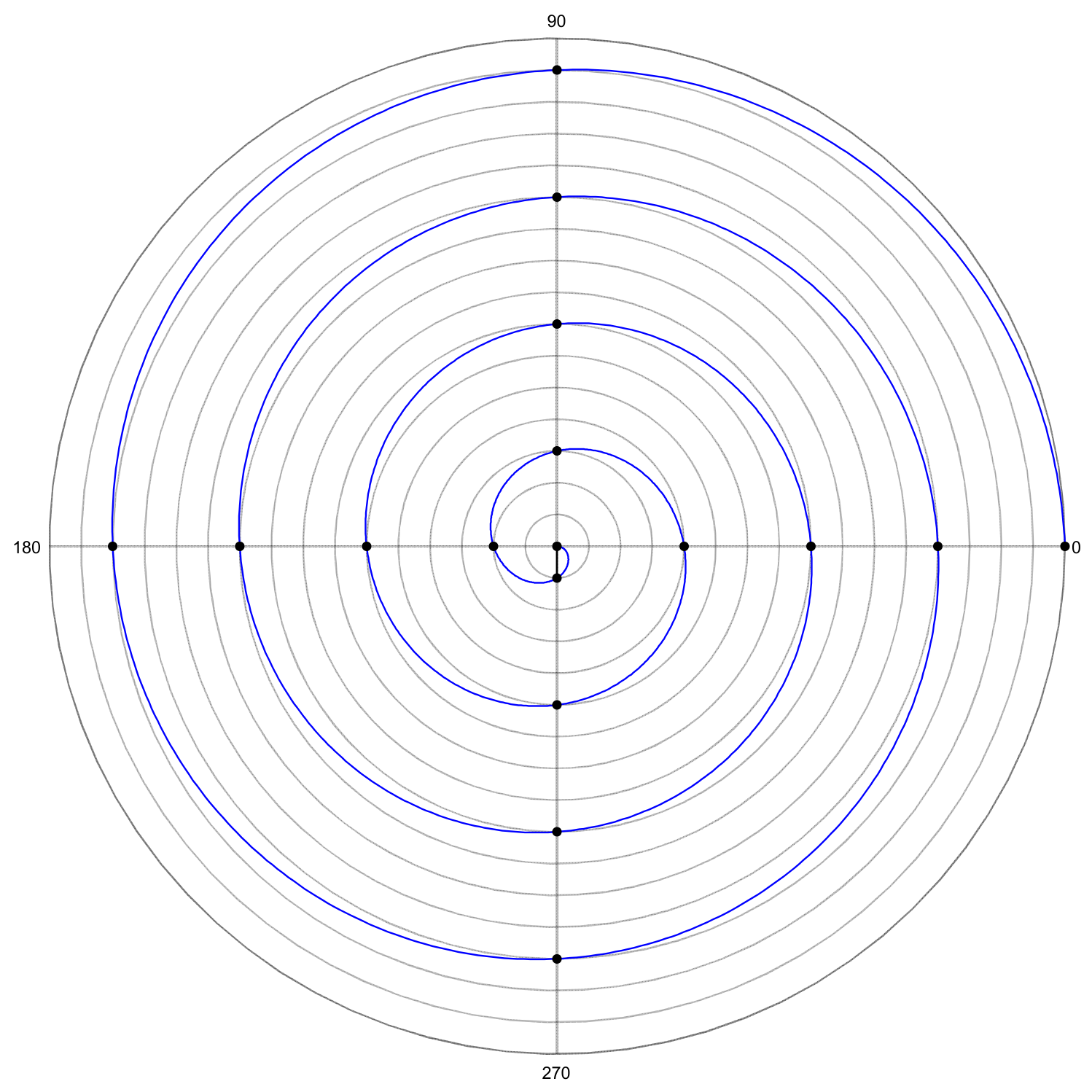
According to Equations (23)–(26), the calculation of CLPs x C L n , c C L m , z L n m m = 1 , 2 , , N p , n = 1 , 2 , , N t in the machining coordinate system can be completed, as shown in Table 6. For the custom discrete spiral trajectory x C L a , c C L a , by interpolating the x C L n , c C L m , z L n m values in Table 6 in accordance with Equations (8)–(17) and the calculation procedure for bicubic spline interpolation functions described in Section 3.3.5 of this paper, the CLPs x C L a , c C L a , z L n a of the custom discrete helical trajectory can be determined. Based on Equations (19) and (20), the total number of CCPs is N t = N p × N s , and the number of control points per helical revolution is N p . Then the number of grid nodes is N p × N t , as shown in Table 6, Figure 8 and Figure 9. The equiangularly discretized helical CLPs can be obtained in the following order:
( c C L 1 , x C L 1 , z L 11 ) ( c C L 2 , x C L 2 , z L 22 ) ( c C L N p , x C L N p , z L N p N p ) ( c C L 1 , x C L ( 1 + N p ) , z L 1 ( 1 + N p ) ) ( c C L 2 , x C L ( 2 + N p ) , z L 2 ( 2 + N p ) ) ( c C L N p , x C L ( 2 N p ) , z L N p ( 2 N p ) ) ( c C L 1 , x C L ( 1 + ( N s 1 ) N p ) , z L 1 ( 1 + ( N s 1 ) N p ) ) ( c C L 2 , x C L ( 2 + ( N s 1 ) N p ) , z L 2 ( 2 + ( N s 1 ) N p ) ) ( c C L N p , x C L N t , z L N p N t )

4. Experiments and Results

The machine tools employed in this research were a Pyramid Nano three-axis milling machine manufactured by Kern (Eschenlohe, Germany) and an IL500 three-axis horizontal diamond lathe manufactured by Innolite (Aachen, Germany). The measurement equipment used was a non-contact profilometer, model NMF350S, manufactured by DUI (Delft, The Netherlands). In the cutting experiments, two diamond ball-end mills manufactured by Yuhe Optical Precision Tools (Shenzhen, China) and four diamond turning tools with a 0° rake angle manufactured by Contour Fine Tooling (Hertfordshire, UK) were used, as listed in Table 7. The diamond ball-end mill designated Q502 has an arc radius of 0.751 mm, and Q503 has an arc radius of 0.742 mm. For the diamond turning tools, cutter SC34435 has a nose arc radius of 1.052 mm and an overall waviness of 40 nm (RMS); cutter SC34439 has a nose arc radius of 2.077 mm and an overall waviness of 35 nm (RMS); cutter SC34436 has a nose arc radius of 1.067 mm and an overall waviness of 22 nm (RMS); and cutter SC34438 has a nose arc radius of 2.009 mm and an overall waviness of 29 nm (RMS).
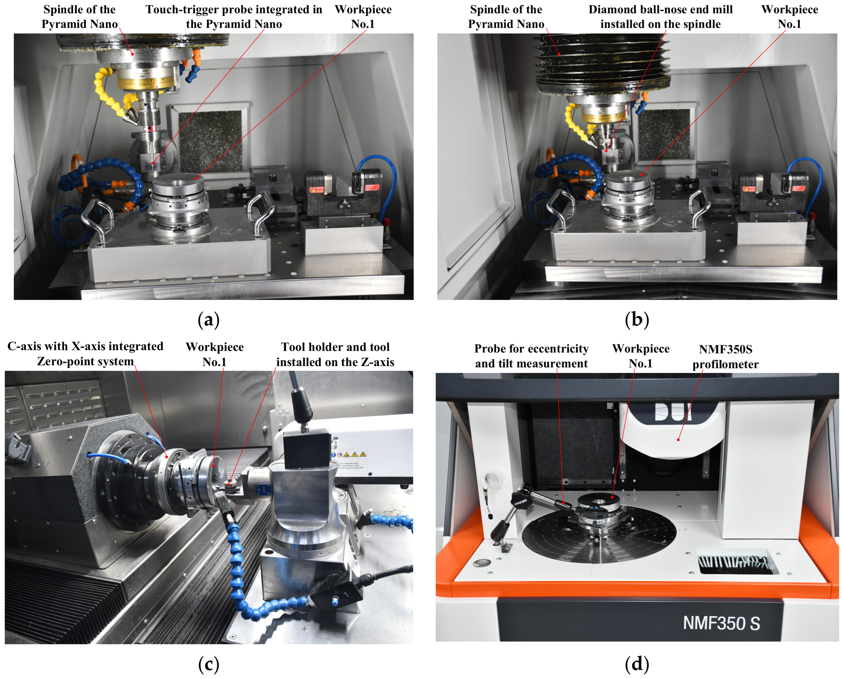
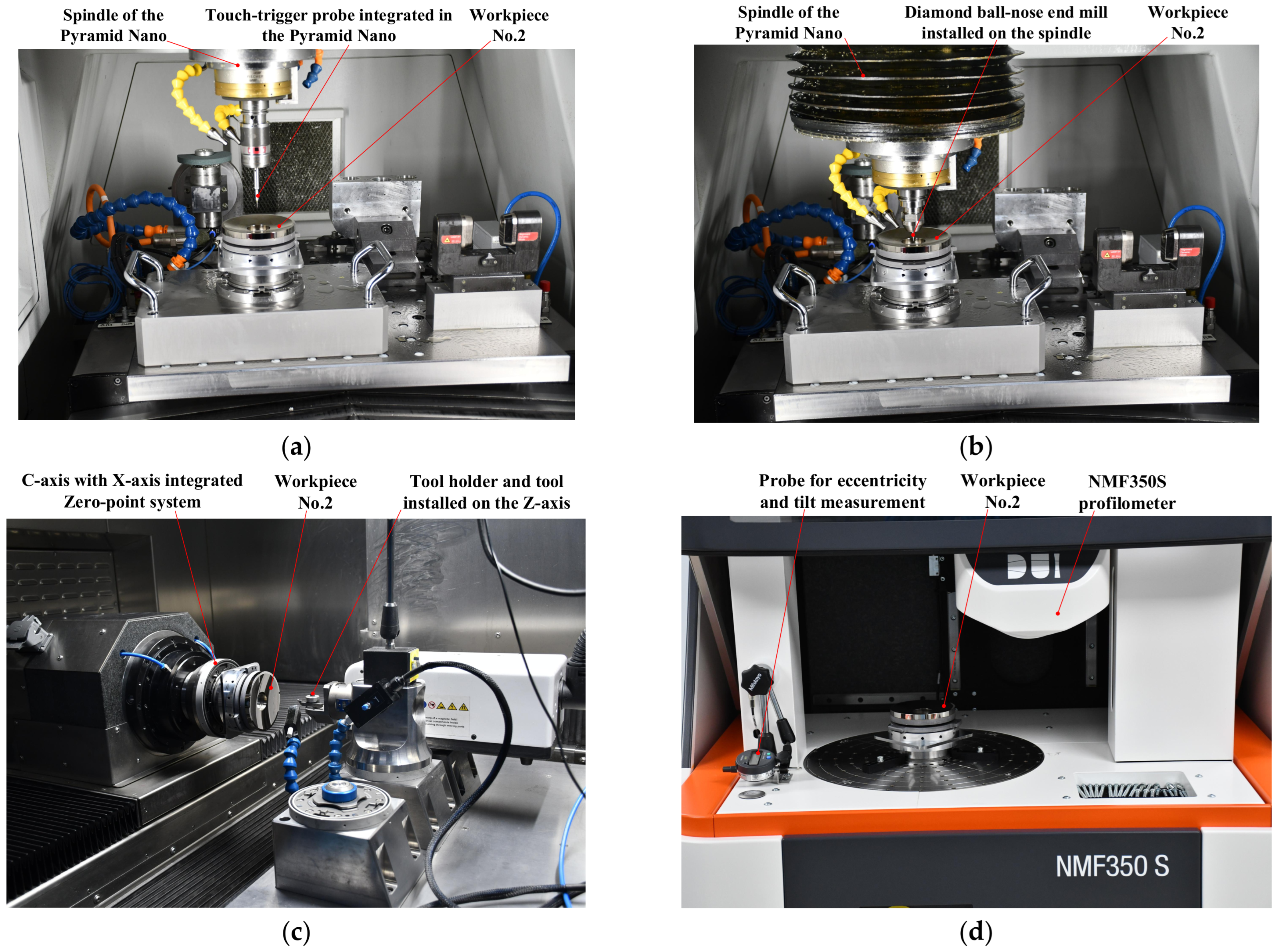
As shown in Figure 6, using the upper end face Ec, the outer cylindrical surface Fc and the fixture side face Gc of the workpiece as reference surfaces, the reference spherical surface of workpiece No. 1 was machined on the Pyramid Nano using a diamond ball-end mill (part number Q502). The freeform surface was then subjected to UP turning, measurement and compensatory machining, as shown in Figure 10.
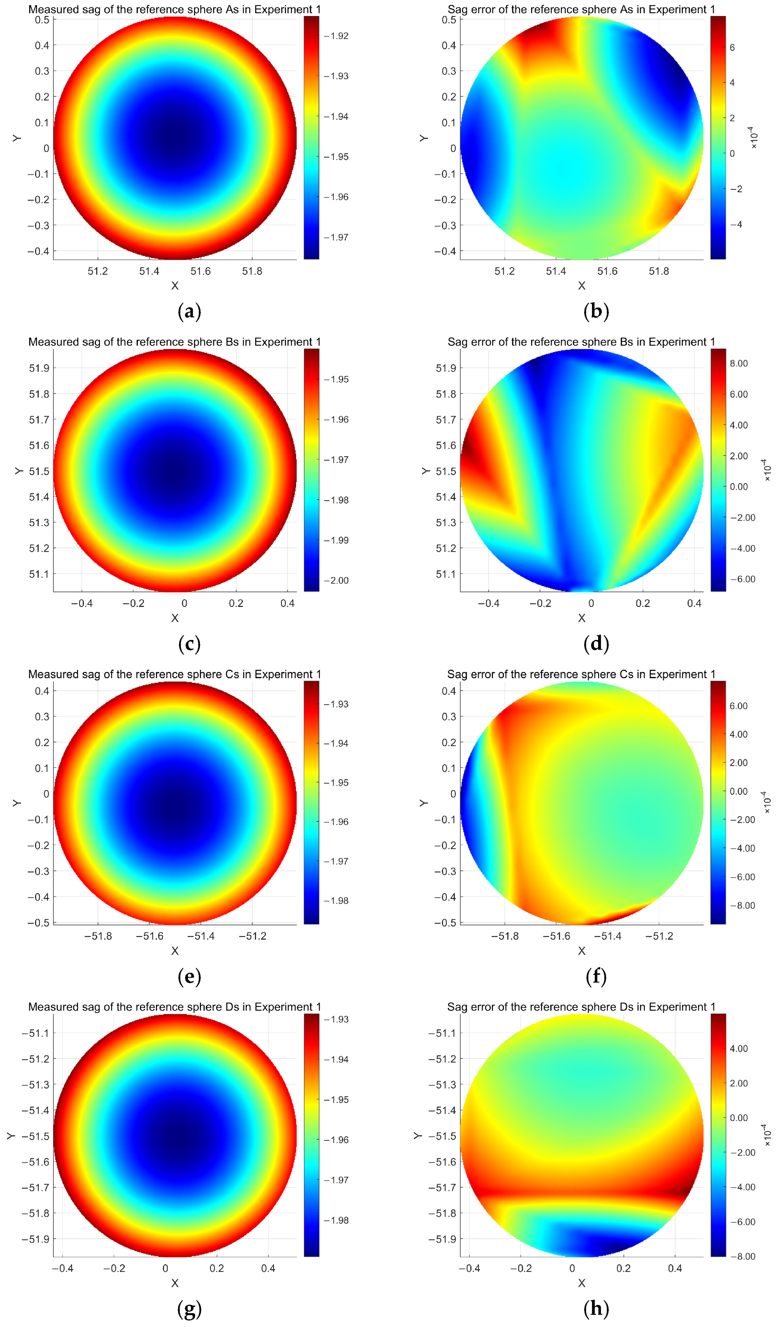
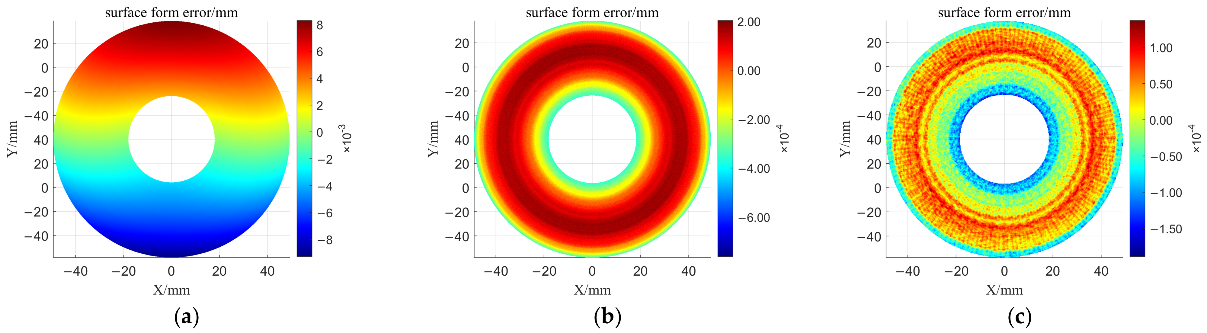
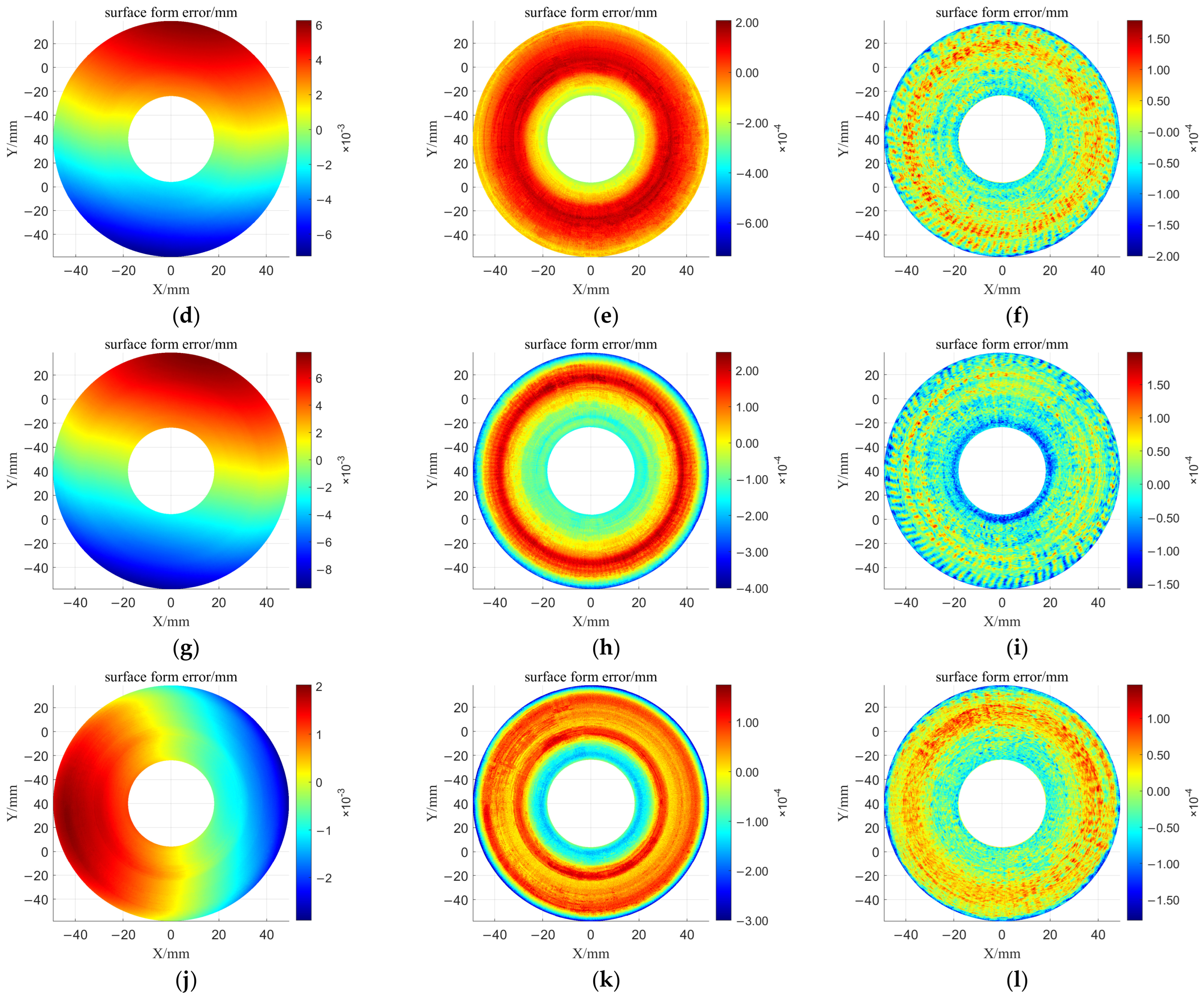
Taking Experiment 1 as an example, based on the measured point clouds of the reference spheres (as illustrated in Figure 11), the positional errors ( T s p x , T s p y ) j j = 1,2 , 3,4 for the reference spheres As, Bs, Cs, and Ds, along with the mounting error R z p of the freeform surface when rotated about the z-axis in the measurement coordinate system, can be obtained by applying the formulas and calculation procedures described in Section 3.1.1, Section 3.1.2 and Section 3.2. The corresponding results are presented in Table 8. Based on the SFE measurement results of the freeform surface without correction for mounting errors, as shown in Figure 12a, the mounting errors T x p , T y p , T z p , R x p and R y p of the freeform surface in the measurement coordinate system can be obtained using the formulae and calculation steps in Section 3.2, as shown in Table 9. Using Equation (16), the SFE of the freeform surface after correction for mounting errors can be obtained, as shown in Figure 12b. Following the theory and algorithms outlined in Section 3.3 and Section 3.4, compensatory machining is performed on the surface; the vector height errors of the freeform surface after compensatory machining are shown in Figure 12c.
This section presents the validation results for the theory and method of error compensation in UP turning of freeform mirrors proposed in this study. A total of eight sets of orthogonal experiments were conducted, with the experimental parameters and results summarized in Table 9. The average SFE of four AlSi40 substrates was improved from RMS 114.8 nm to RMS 47.9 nm, whilst that of four AlSi40 substrates with NiP-plated surfaces was improved from RMS 71.3 nm to RMS 31.1 nm.
The experimental parameters and results are presented in Table 9. Experiments 1–4 were conducted on workpiece No. 1 (made of AlSi40). In Experiment 1, the surface form accuracy before compensation was 151.8 nm (RMS), which improved to 54.1 nm (RMS) after compensation. In Experiment 2, the accuracy before and after compensation was 100.4 nm (RMS) and 49.6 nm (RMS), respectively. In Experiment 3, the corresponding values were 119.6 nm (RMS) and 44.1 nm (RMS). In Experiment 4, the accuracy before and after compensation was 87.4 nm (RMS) and 43.9 nm (RMS), respectively. The SFE distributions before and after compensation are shown in Figure 12.
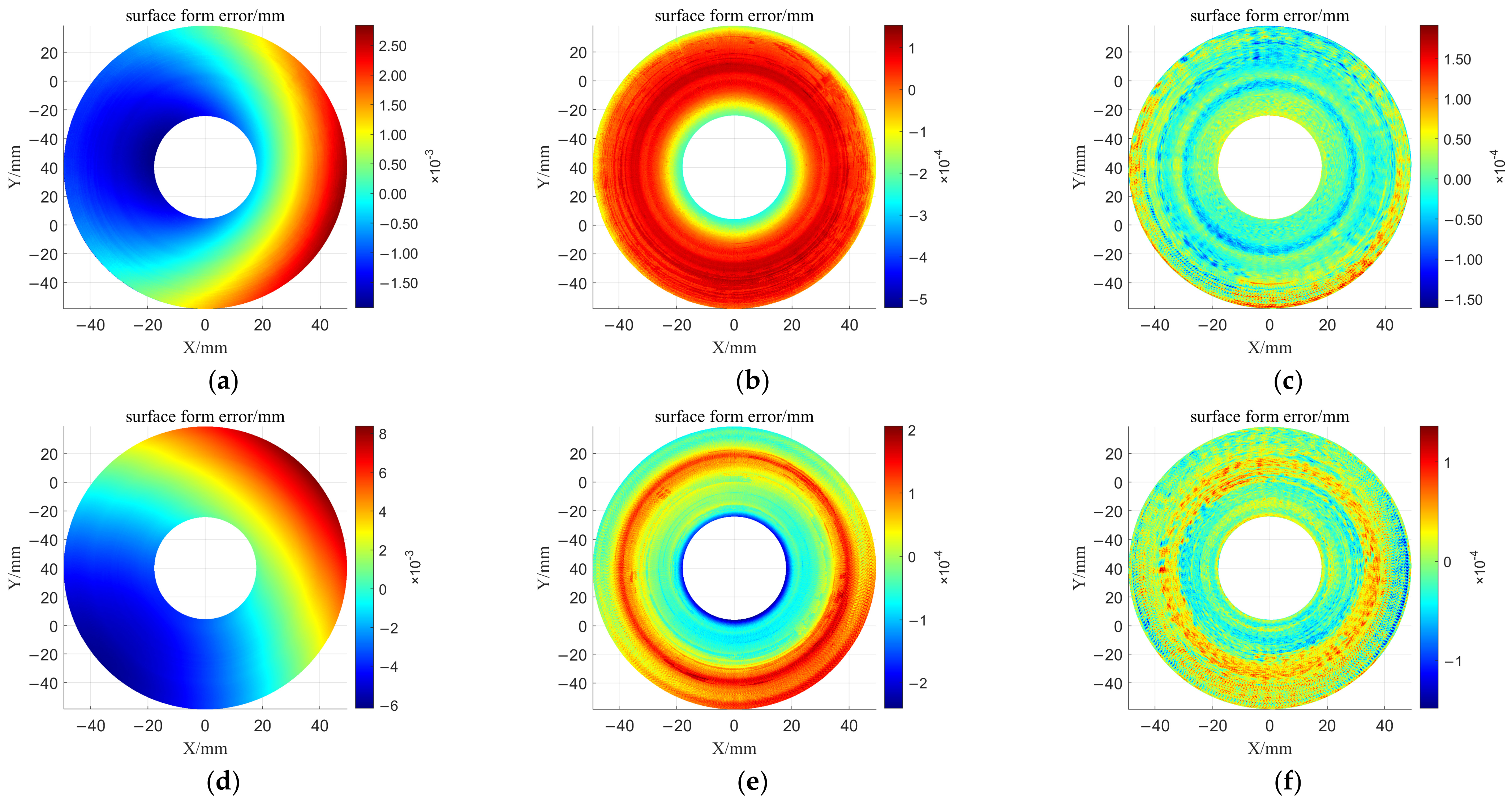
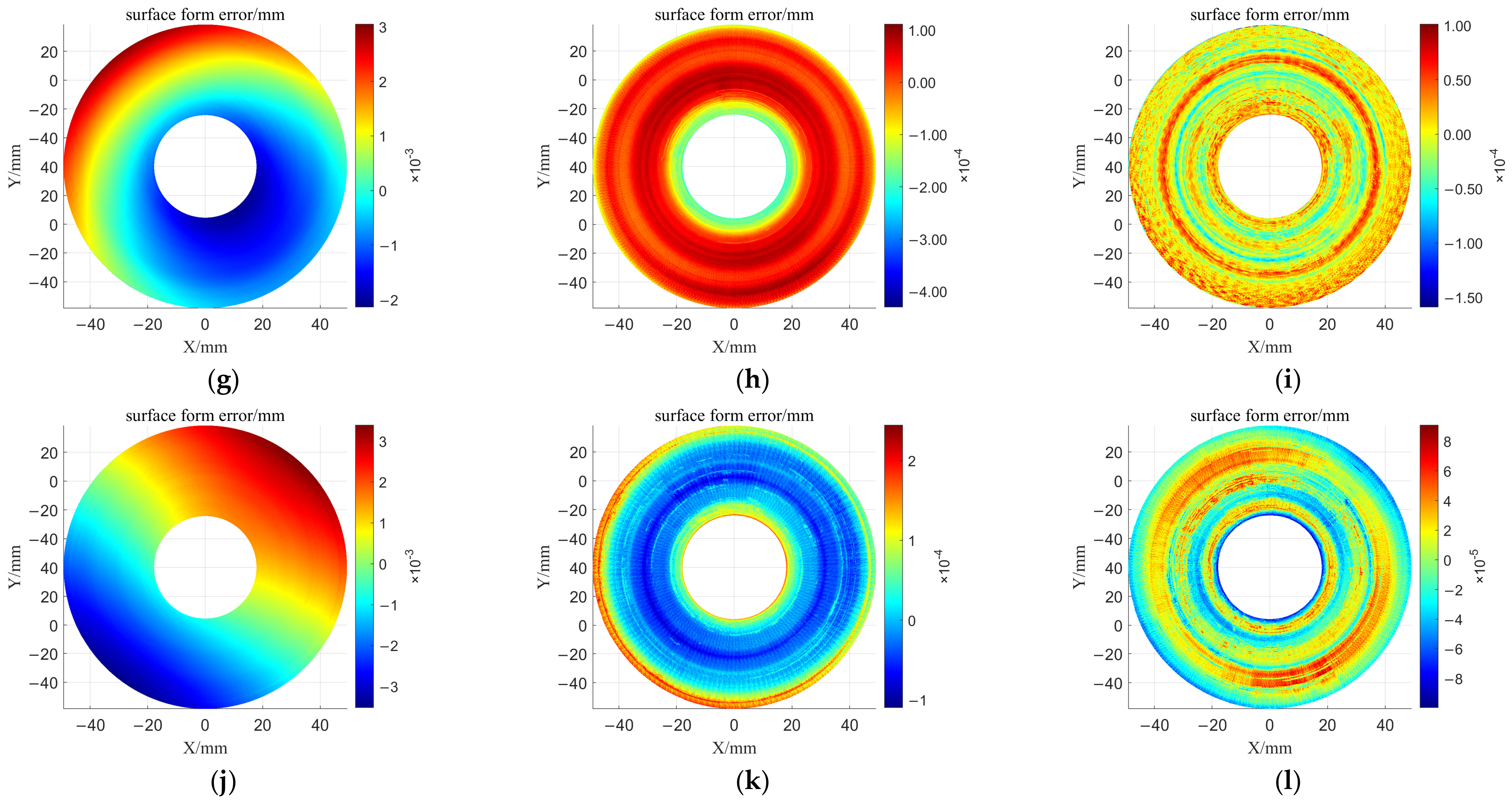
As shown in Figure 6, using the upper end face Ec, the outer cylindrical surface Fc of the workpiece, and the side surface Gc of the fixture as references, the reference spherical surface of workpiece No. 2 was machined on a Pyramid Nano using a diamond ball-end mill with the designation Q503. Subsequently, UP turning, measurement, and compensation machining of the freeform surface were performed, as illustrated in Figure 13. The experimental parameters and results are presented in Table 9. Experiments 5–8 were conducted on workpiece No. 2 (AlSi40 substrates with NiP-plated surfaces). In Experiment 5, the surface form accuracy before compensation was 82.9 nm (RMS), which improved to 36.1 nm (RMS) after compensation. In Experiment 6, the accuracy before and after compensation was 77.1 nm (RMS) and 33.1 nm (RMS), respectively. In Experiment 7, the corresponding values were 63.4 nm (RMS) and 27.2 nm (RMS). In Experiment 8, the accuracy before and after compensation was 61.9 nm (RMS) and 28.0 nm (RMS), respectively. The SFEs before and after compensation are shown in Figure 14.

5. Discussion

To address the limitations of existing compensation methods for SFE on freeform surfaces, this study presents a novel approach for error calculation and compensation using measurement data acquired from a non-contact profilometer. By designing reference spheres and utilizing the measured point clouds from reference spheres, the mounting error R z p of the freeform surface in the measurement coordinate system was calculated. Based on the sag error measurement data of the freeform surface, the mounting pose errors T x p , T y p , T z p , R x p and R y p in the measurement coordinate system were calculated using the least squares method, and the measurement error caused by these errors was corrected. Subsequently, Makima bicubic spline interpolation and coordinate transformation methods were employed to convert the SFE of the freeform surface in the measurement coordinate system into machining error in the machining coordinate system. The machining error was then compensated for in the planned mesh surface point cloud, and the CLPs were determined using an iterative solution based on the bisection method with piecewise cubic spline fitting.
As illustrated in Figure 11, the freeform surface and the reference spheres were fabricated on separate machine tools. The average RMS sag error for the reference spheres is approximately 300 nanometers, as presented in Figure 10 and Table 7. If an UP milling spindle could be integrated into a UP lathe, both the freeform surface and the reference spheres could be machined directly on the same platform, thereby mitigating the effects of uncertainty propagation. Moreover, by further reducing the waviness error of the ball-end mill, the calculation accuracy of the mounting error R z p could be further enhanced.
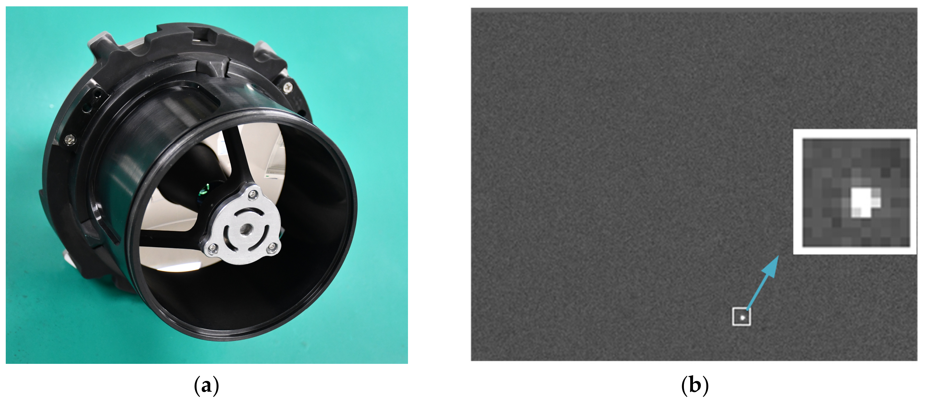
In terms of SFE compensation accuracy, the machining accuracy of the NiP-plated surfaces improved from an average RMS of 71.3 nm to 31.1 nm. Following compensation, the surface meets the accuracy requirements for optical systems used in near-infrared star tracking without the need for polishing, thereby significantly enhancing the manufacturing precision and efficiency of freeform surfaces. By further controlling tool waviness errors, it is anticipated that the accuracy of the compensation machining can be improved. In terms of optical performance, experimental verification has shown that the system’s star-tracking performance reaches +0.54 magnitudes (as shown in Figure 15).

6. Conclusions

Compared with the CGH method, using a profilometer to measure freeform surfaces offers significant advantages in terms of high efficiency. Addressing the manufacturing requirements of freeform mirrors for the near-infrared stellar tracker optical system, as well as the considerable room for further improvement in both accuracy and manufacturing efficiency of existing UP turning error compensation methods for complex surfaces reported in the literature, this study proposes and validates a novel compensation method. Through experimental validation, the following conclusions are drawn.
(1) A method is proposed that employs point clouds of the reference spherical surfaces and the form error of the freeform surface measured by a profilometer to calculate the mounting pose errors of the workpiece on the profilometer based on the least squares method. This approach resolves the current limitation of profilometers in determining the mounting pose errors of the freeform surface in the measurement coordinate system, thereby avoiding measurement error induced by mounting pose errors and improving the reliability of freeform surface form accuracy measurement.
(2) A method is proposed that generates an isometric polar coordinate grid and calculates the freeform surface point cloud corrected for machining error. The machining error in the machining coordinate system is obtained from the form error in the measurement coordinate system of the freeform surface using Makima bicubic spline interpolation and coordinate transformation. The machining error is then compensated into the generated grid surface point cloud, followed by the determination of CLPs through piecewise cubic spline fitting. This method addresses the issue of mapping error inherent in directly mapping the SFE to CLPs as reported in the existing literature.
(3) An algorithm based on the bisection method is proposed to iteratively calculate the CLPs in UP turning. This algorithm maintains consistency between the x-coordinate of the CLPs and the planned tool path, thereby ensuring steady X movement during machining and ensuring the accuracy of CLPs calculation.
(4) Using the method proposed in this study, the average SFE of four AlSi40 substrates was improved from RMS 114.8 nm to RMS 47.9 nm, whilst that of four AlSi40 substrates with NiP-plated surfaces was improved from RMS 71.3 nm to RMS 31.1 nm. Following compensation, the surface profile accuracy requirements for optical systems used in near-infrared stellar tracker can be met without the need for polishing, whilst significantly improving the manufacturing efficiency of freeform mirrors.
The measurement and compensation methods proposed in this study provide an efficient and high-precision solution for error compensation in the UP turning of complex-surface mirrors. In the future, by further controlling tool waviness errors, it is expected that compensation accuracy can be further enhanced, thereby expanding its applications in various imaging and laser systems.

Author Contributions

Experiment and verification, Y.P.; writing, manuscript, Y.P.; conceptualization, H.D.; visualization, L.M.; data curation, Q.C.; investigation, Y.Y.; resources, M.L.; supervision, F.F.; funding acquisition and methodology, D.Z. All authors have read and agreed to the published version of the manuscript.

Funding

This research was funded by the National Natural Science Foundation of China (No. 52375431 and No. 42204182) and the Huazhong Institute of Electro-Optics (No. M1-8004-2311-1).

Institutional Review Board Statement

Not applicable.

Informed Consent Statement

Not applicable.

Data Availability Statement

Data will be made available on request.

Acknowledgments

We thank the staff in our laboratory, Mingming Sha, for his help with the experiment.

Conflicts of Interest

The authors declare no conflicts of interest.

References

  1. Peng, L.; Li, X.; Li, L.; Cheng, Q.; Luo, X.; Zhou, X.; Zhang, X. Application of the Improved Grinding Technology to Freeform Surface Manufacturing. Photonics 2023, 10, 240. [Google Scholar] [CrossRef]
  2. Zhu, W.L.; Beaucamp, A. Compliant grinding and polishing: A review. Int. J. Mach. Tools Manuf. 2020, 158, 103634. [Google Scholar] [CrossRef]
  3. Wang, J.; Wang, X.; Peng, L.; Wang, J.; Liu, Z.; Li, L.; Cai, M.; Liu, B.; Li, W.; Zhang, X. Method for testing freeform surfaces based on a Shack-Hartmann sensor with plane wavefront scanning and stitching. Opt. Express 2023, 31, 36702–36724. [Google Scholar] [CrossRef] [PubMed]
  4. Fang, F.Z.; Zhang, X.D.; Weckenmann, A.; Zhang, G.X.; Evans, C. Manufacturing and measurement of freeform optics. Cirp Ann. 2013, 62, 823–846. [Google Scholar] [CrossRef]
  5. Yang, T.; Jin, G.F.; Zhu, J. Automated design of freeform imaging systems. Light Sci. Appl. 2017, 6, e17081. [Google Scholar] [CrossRef] [PubMed]
  6. Chen, S.; Xue, S.; Zhai, D.; Tie, G. Measurement of freeform optical surfaces: Trade-off between accuracy and dynamic range. Laser Photonics Rev. 2020, 14, 1900365. [Google Scholar] [CrossRef]
  7. Rolland, J.P.; Davies, M.A.; Suleski, T.J.; Evans, C.; Bauer, A.; Lambropoulos, J.C.; Falaggis, K. Freeform optics for imaging. Optica 2021, 8, 161–176. [Google Scholar] [CrossRef]
  8. Tian, Y.; Qiao, S.; Guo, S.; Hou, Y.; Shi, F. Combined polishing process of a sapphire aspherical component based on temperature-controlled magnetorheological processing. Appl. Opt. 2023, 62, 805–812. [Google Scholar] [CrossRef] [PubMed]
  9. Venditti, K.; Evans, C.; Falaggis, K.; Blum, A.; Chaudhuri, R.; Goodsell, J.; Rolland, J.P. Design for metrology for freeform optics manufacturing. Procedia CIRP 2019, 84, 169–172. [Google Scholar] [CrossRef]
  10. Rolland, J.P.; Fuerschbach, K.; Davis, G.E.; Thompson, K.P. Pamplemousse: The Optical Design, Fabrication, and Assembly of a Three-Mirror Freeform Imaging Telescope. In Proceedings of the International Optical Design Conference 2014; SPIE: Bellingham, WA, USA, 2014; pp. 172–177. [Google Scholar]
  11. Fuerschbach, K.; Davis, G.E.; Thompson, K.P.; Rolland, J.P. Assembly of a freeform off-axis optical system employing three φ-polynomial Zernike mirrors. Opt. Lett. 2014, 39, 2896–2899. [Google Scholar] [CrossRef] [PubMed]
  12. Deng, Y.; Tan, Y.; Wu, X.; Zhu, J. Local tolerance and quality evaluation for optical surfaces. Optica 2022, 9, 1039–1049. [Google Scholar] [CrossRef]
  13. Kumar, S.; Zhong, W.; Williamson, J.; Kumar, P.; Furness, T.; Lou, S.; Zeng, W.; Jiang, X. Design, fabrication, and testing of freeform mirror-based head-up display system. Opt. Laser Technol. 2025, 186, 112653. [Google Scholar] [CrossRef]
  14. Hilpert, E.; Hartung, J.; von Lukowicz, H.; Herffurth, T.; Heidler, N. Design, additive manufacturing, processing, and characterization of metal mirror made of aluminum silicon alloy for space applications. Opt. Eng. 2019, 58, 092613. [Google Scholar] [CrossRef]
  15. Feigl, T.; Perske, M.; Pauer, H.; Fiedler, T.; Zeitner, U.; Leitel, R.; Eckstein, H.C.; Schleicher, P.; Schröder, S.; Trost, M.; et al. Sub-Aperture EUV Collector with Dual-Wavelength Spectral Purity Filter. In Proceedings of the Extreme Ultraviolet (EUV) Lithography VI; SPIE: Bellingham, WA, USA, 2015; pp. 95–101. [Google Scholar]
  16. Heidler, N.; Hilpert, E.; Hartung, J.; Von Lukowicz, H.; Damm, C.; Peschel, T.; Risse, S. Additive Manufacturing of Metal Mirrors for TMA Telescope. In Proceedings of the Optical Fabrication, Testing, and Metrology VI; SPIE: Bellingham, WA, USA, 2018; pp. 92–98. [Google Scholar]
  17. Risse, S.; Kinast, J.; Gebhardt, A.; Jende, R.; Kleinbauer, K.; Müller, S.; Peschel, T.; Damm, C.; Schwarzenberg, M.; Kroedel, M.; et al. Ultraprecise Flat Mirrors for the Pointing Unit of the DESIS Instrument on Board of the ISS. In Proceedings of the Material Technologies and Applications to Optics, Structures, Components, and Sub-Systems IV; SPIE: Bellingham, WA, USA, 2019; pp. 41–52. [Google Scholar]
  18. Rohloff, R.R.; Gebhardt, A.; Schönherr, V.; Risse, S.; Kinast, J.; Scheiding, S.; Peschel, T. A Novel Athermal Approach for High-Performance Cryogenic Metal Optics. In Proceedings of Modern Technologies in Space- and Ground-Based Telescopes and Instrumentation; SPIE: Bellingham, WA, USA, 2010; pp. 1526–1539. [Google Scholar]
  19. Schürmann, M.; Risse, S.; Kämmer, H.; Franke, C.; Schlegel, R.; Müller, S.; Kaiser, N. Metal Mirrors with Metal-Dielectric HR-Coating for Ultrashort Laser Pulses Applied in Scanner Applications. In Proceedings of Laser-Based Micro- and Nanoprocessing IX; SPIE: Bellingham, WA, USA, 2015; pp. 155–165. [Google Scholar]
  20. Arcangeli, L.; Bianucci, G.; Marioni, F.; Mazzoleni, R.; Rossi, M.; Terraneo, M.; Zocchi, F.E.; Meini, M.; Galeotti, M.; Gabrieli, R.; et al. Manufacturing and Qualification of the QM Mirror for the High-Resolution Spectrometer of the FLEX Mission. In Proceedings of the International Conference on Space Optics (ICSO 2018); SPIE: Bellingham, WA, USA, 2019; pp. 3065–3071. [Google Scholar]
  21. Rahman, S.K.S.U.; Wieland, H.U.; Burstein, V.; Hübner, M. High-Performance All-Metal Telescope for Satellite-Based Laser Communication Terminals. In Proceedings of Sensors and Systems for Space Applications XV; SPIE: Bellingham, WA, USA, 2022; pp. 153–167. [Google Scholar]
  22. Scheiding, S.; Stenzel, O.; Gliech, S. Metal Mirrors with Excellent Figure and Roughness. In Proceedings of SPIE; SPIE: Bellingham, WA, USA, 2008; pp. 317–347. [Google Scholar]
  23. von Lukowicz, H.; Hartung, J.; Hilpert, E.; Damm, C.; Peschel, T.; Heidler, N. Optimization and Additive Manufacturing of a Three-Mirror-Anastigmatic Telescope. In Proceedings of the International Conference on Space Optics (ICSO 2020); SPIE: Bellingham, WA, USA, 2021; pp. 67–78. [Google Scholar]
  24. Horvath, N.W.; Davies, M.A. Concurrent Engineering of a Next-Generation Freeform Telescope: Mechanical Design and Manufacture. In Proceedings of Advanced Optics for Imaging Applications: UV Through LWIR IV; SPIE: Bellingham, WA, USA, 2019; pp. 140–147. [Google Scholar]
  25. Lee, W.B.; Cheung, C.F.; Chiu, W.M.; Chiu, W.M.; Leung, T.P. An investigation of residual form error compensation in the ultra-precision machining of aspheric surfaces. J. Mater. Process. Technol. 2000, 99, 129–134. [Google Scholar] [CrossRef]
  26. Nagayama, K.; Yan, J. Deterministic error compensation for slow tool servo-driven diamond turning of freeform surface with nanometric form accuracy. J. Manuf. Process. 2021, 64, 45–57. [Google Scholar] [CrossRef]
  27. Parker, R.A.; Hedges, A.R.; Holt, D.J.; Myler, J.K. Tool Geometry and Wear Effects in Diamond Turning. In Proceedings of Infrared Technology and Applications; SPIE: Bellingham, WA, USA, 1990; pp. 341–352. [Google Scholar]
  28. Peng, Y.; Ding, H.; Zhang, D.; Luo, M. Calculation of Tool Offset and Tool Radius Errors Based on On-Machine Measurement and Least Squares Method in Ultra-Precision Diamond Turning. Photonics 2024, 11, 1022. [Google Scholar] [CrossRef]
  29. Nagayama, K.; Yan, J. Measurement and compensation of tool contour error using white light interferometry for ultra-precision diamond turning of freeform surfaces. Int. J. Autom. Technol. 2020, 14, 654–664. [Google Scholar] [CrossRef]
  30. Liang, R.; Yu, Y.; Chen, J.; Zhang, X.; Ren, M.; Huang, N.; Zhu, L. Tool path generation with a uniform residual error distribution considering tool contour error for ultra-precision diamond turning. J. Manuf. Process. 2024, 115, 466–480. [Google Scholar] [CrossRef]
  31. Zhang, X.; Wu, H.; Yu, Y.; Jia, Z.; Wang, X.; Ren, M.; Zhu, L. Model-free tool path modification in ultra-precision diamond turning of freeform surfaces using iterative learning control. Precis. Eng. 2025, 94, 736–748. [Google Scholar] [CrossRef]
  32. Hashimoto, T.; Yan, J. Time delay compensation in high-speed diamond turning of freeform surface using independent fast tool servo with a long stroke. Precis. Eng. 2025, 93, 515–527. [Google Scholar] [CrossRef]
  33. Hopper, L.; Noste, T.; Miller, J.; Evans, C. Error Sources, Compensation, and Probe Path Optimization for On-Machine Metrology of Freeform Optics. In Proceedings of Optical Manufacturing and Testing XIII; SPIE: Bellingham, WA, USA, 2020; pp. 39–49. [Google Scholar]
  34. He, S.; Wu, J.; Xuan, J.; Du, W.; Xia, Q.; Zhang, L.; Xiong, S.; Shi, T. Freeform surface topography model for ultraprecision turning under the influence of various errors. J. Manuf. Process. 2021, 71, 429–449. [Google Scholar] [CrossRef]
  35. Chen, S.; Guan, C.; Hu, H.; Hu, H.; Xue, S.; Dai, Y. Corrective machining of monolithic multiple freeform mirrors based on holographic null test. Opt. Lasers Eng. 2023, 170, 107789. [Google Scholar] [CrossRef]
  36. Chen, S.; Hu, H.; Guan, C. Fiducial free correction of mapping distortion in null test of aspheres and freeforms. Opt. Commun. 2022, 506, 127560. [Google Scholar] [CrossRef]
  37. Wang, C.; Xu, K.; Sun, X.; Bian, X.; Zhong, H.; Zhang, Z.; Deng, W.; Zhang, X.; Yan, J. On-machine measurement and Zernike-based compensation cutting for large-aperture additive metal mirrors with ultra-high lightweight ratio. Opt. Express 2025, 33, 36930–36942. [Google Scholar] [CrossRef] [PubMed]
  38. Yu, J.; Mao, X.; Gao, R.; Li, J.; Wang, P.; Xu, Z.; Yuan, Y.; Wang, F. Unobscured off-axis three-mirror freeform all-aluminum imaging telescope. Appl. Opt. 2025, 64, 1677–1692. [Google Scholar] [CrossRef]
  39. Zhu, Z.; To, S. Adaptive tool servo diamond turning for enhancing machining efficiency and surface quality of freeform optics. Opt. Express 2015, 23, 20234–20248. [Google Scholar] [CrossRef] [PubMed]
  40. He, S.; Xuan, J.; Du, W.; Xia, Q.; Xiong, S.; Zhang, L.; Wang, Y.; Wu, J.; Tao, H.; Shi, T. Spiral tool path generation method in a NURBS parameter space for the ultra-precision diamond turning of freeform surfaces. J. Manuf. Process. 2020, 60, 340–355. [Google Scholar] [CrossRef]
  41. You, K.; Yan, G.; Fang, F.; Li, Z.; Zhang, Y. Tool path generation of turning optical freeform surfaces using arbitrary rake angle tools. Opt. Express 2020, 28, 38252–38266. [Google Scholar] [CrossRef] [PubMed]
  42. Ao, S.; Gong, H.; Huang, K. A smooth tool path generation method for ultraprecision turning discontinuous multi-freeform-surfaces with high machining efficiency. J. Mater. Process. Technol. 2021, 298, 117280. [Google Scholar] [CrossRef]
  43. Guo, Y.; Yang, X.; Kang, J.; Yao, T.; Cheng, B.; Li, M.; Xie, Q. Spiral tool path optimization method for fast/slow tool servo-assisted diamond turning of freeform surfaces with highly form accuracy. Precis. Eng. 2023, 80, 229–242. [Google Scholar] [CrossRef]
  44. Buhmann, M.; Carelli, E.; Egger, C.; Frick, K. Point cloud based tool path generation for corrective machining in ultra-precision diamond turning. Int. J. Adv. Manuf. Technol. 2022, 120, 6891–6907. [Google Scholar] [CrossRef]
  45. Spong, M.W.; Hutchinson, S.; Vidyasagar, M. Robot Modeling and Control; Wiley: New York, NY, USA, 2020. [Google Scholar]
  46. Sauer, T. Numerical Analysis; Pearson: New York, NY, USA, 2019. [Google Scholar]
  47. Ionita, C.; Moler, C. Makima Piecewise Cubic Interpolation. Blog Post, 2019, 29. Available online: https://blogs.mathworks.com/cleve/2019/04/29/makima-piecewise-cubic-interpolation/ (accessed on 20 April 2026).
Figure 1. Manufacturing Process for AlSi40 mirrors.
Photonics 13 00580 g001
Figure 2. Layout of the unobscured stellar tracker optical system.
Photonics 13 00580 g002
Figure 3. Spot diagrams for different field positions.
Photonics 13 00580 g003
Figure 4. Encircled energy.
Photonics 13 00580 g004
Figure 5. Metallographic image of the AlSi40.
Photonics 13 00580 g005
Figure 6. Schematic of the M1 machining and measurement datum (with fixture and flange). (a) Axonometric view; (b) front view; (c) left sectional view.
Photonics 13 00580 g006
Figure 7. Method for compensating for form errors in UP turning of freeform surfaces.
Photonics 13 00580 g007
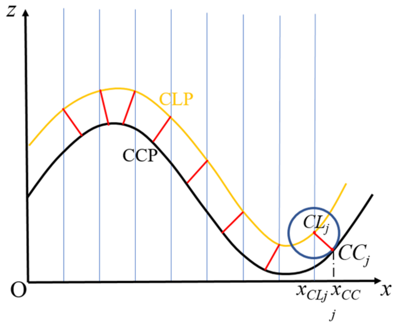
Figure 8. Schematic diagram of CCP and CLP.
Photonics 13 00580 g008
Figure 9. Schematic diagram of equiangularly discretized spiral on a polar coordinate grid.
Photonics 13 00580 g009
Figure 10. (a) Set up the machining coordinate system for workpiece No. 1 on the Pyramid Nano; (b) machining the reference spheres for workpiece No. 1; (c) machining the freeform surface of workpiece No. 1 on the IL500; (d) measuring the freeform surface of workpiece No. 1 on the NMF350S.
Photonics 13 00580 g010
Figure 11. (a) Measured point clouds of the reference sphere As in Experiment 1; (b) measured sag error of the reference sphere As in Experiment 1; (c) measured point clouds of the reference sphere Bs in Experiment 1; (d) measured sag error of the reference sphere Bs in Experiment 1; (e) measured point clouds of the reference sphere Cs in Experiment 1; (f) measured sag error of the reference sphere Cs in Experiment 1; (g) measured point clouds of the reference sphere Ds in Experiment 1; (h) measured sag error of the reference sphere Ds in Experiment 1.
Photonics 13 00580 g011
Figure 12. (a) SFE before removing measurement error in Experiment 1; (b) SFE after removing measurement error in Experiment 1; (c) SFE after compensation in Experiment 1; (d) SFE before removing measurement error in Experiment 2; (e) SFE after removing measurement error in Experiment 2; (f) SFE after compensation in Experiment 2; (g) SFE before removing measurement error in Experiment 3; (h) SFE after removing measurement error in Experiment 3; (i) SFE after compensation in Experiment 3; (j) SFE before removing measurement error in Experiment 4; (k) SFE after removing measurement error in Experiment 4; (l) SFE after compensation in Experiment 4.
Photonics 13 00580 g012aPhotonics 13 00580 g012b
Figure 13. (a) Establish the machining coordinate system for workpiece No. 2 on the Pyramid Nano; (b) machine the reference spheres for workpiece No. 2; (c) machine the freeform surface of workpiece No. 2 on the IL500; (d) measure the freeform surface of workpiece No. 2 on the NMF350S.
Photonics 13 00580 g013
Figure 14. (a) SFE before removing measurement error in Experiment 5; (b) SFE after removing measurement error in Experiment 5; (c) SFE after compensation in Experiment 5; (d) SFE before removing measurement error in Experiment 6; (e) SFE after removing measurement error in Experiment 6; (f) SFE after compensation in Experiment 6; (g) SFE before removing measurement error in Experiment 7; (h) SFE after removing measurement error in Experiment 7; (i) SFE after compensation in Experiment 7; (j) SFE before removing measurement error in Experiment 8; (k) SFE after removing measurement error in Experiment 8; (l) SFE after compensation in Experiment 8.
Photonics 13 00580 g014aPhotonics 13 00580 g014b
Figure 15. (a) Photograph of the stellar tracker optical system; (b) point-source image test result at a magnitude of +0.54.
Photonics 13 00580 g015
Table 1. Main technical specifications of the stellar tracker optical system.
ParameterSpecification
Wavelength/nm1360~1700 nm
Focal length1500 mm
Entrance pupil diameter/mm98
Pixel size30 μm × 30 μm
Pixel number320 × 256
MTF@17 lp/mm>0.3
Table 2. Technical parameters of the freeform primary and secondary mirrors.
Mirror R 0 /mmkClear Aperture/mmmn C ( m , n ) Form Error Tolerance RMS/nm
M1−154.6−19820−4.185937 × 10⁻⁸≤50
02−2.139926 × 10⁻⁷
40−9.012077 × 10⁻¹²
228.712193 × 10⁻¹¹
043.990096 × 10⁻¹¹
M2−44.77−2.51723.520−1.004846 × 10⁻⁷≤37.5
02−4.442221 × 10⁻⁶
40−3.207626 × 10⁻⁹
223.064247 × 10⁻⁸
041.430809 × 10⁻⁸
Table 3. 80% energy diffusion spot diameter in each field of view (FOV).
Field of View (FOV)Diffusion Spot Diameter/μm
044.270
−0.7 × FOV46.796
0.7 × FOV46.719
−1 × FOV57.320
1 × FOV57.333
Table 4. Parts used in this research.
PartsMaterialSurface GeometryClear ApertureMaterial Blank Supplier
workpiece No. 1AlSi40M198 mmIMR
workpiece No. 2NiP plated on AlSi40M198 mmIMR
Table 5. CCPs x C L n , c C L m , z C n m on the polar coordinate grid in the machining coordinate system.
xCL1xCL2 xCLn
cCL1zC11zC21 zCn1
cCL2zC12zC22 zCn2
cCLmzC1mzC2m zCnm
Table 6. CLPs x C L n , c C L m , z L n m on the polar coordinate grid in the machining coordinate system.
xCL1xCL2 x C L N p
cCL1zL11zL21 zLn1
cCL2zL12zL22 ZLn2
c C L N t zL1mzL2m zLnm
Table 7. Equipment and tools used in this research.
EquipmentModel NO.ManufacturerMain Technical Parameters
Milling machinePyramid NanoKern (Eschenlohe, Germany)Positioning accuracy ≤ 1.5 μm
Horizontal latheIL500Innolite (Aachen, Germany)C-axis runout < 15 nm
ProfilometerNMF350SDUI (Delft, the Netherlands)Measurement accuracy of freeform surfaces < RMS 15 nm
Diamond ball-nose end millQ502Yuhe Optical Precision Tools (Shenzhen, China)Arc radius: 0.751 mm
Diamond ball-nose end millQ503Yuhe Optical Precision Tools (Shenzhen, China)Arc radius: 0.42 mm
Diamond toolSC34435Contour Fine Tooling (Hertfordshire, UK)Rake angle: 0°, arc radius: 1.052 mm, overall waviness: 40 nm
Diamond toolSC34439Contour Fine Tooling (Hertfordshire, UK)Rake angle: 0°, arc radius: 2.077 mm, overall waviness: 35 nm
Diamond toolSC34436Contour Fine Tooling (Hertfordshire, UK)Rake angle: 0°, arc radius: 1.067 mm, overall waviness: 22 nm
Diamond toolSC34438Contour Fine Tooling (Hertfordshire, UK)Rake angle: 0°, arc radius: 2.009 mm, overall waviness: 29 nm
Table 8. Positional errors of the reference spheres and mounting pose error of the freeform surface.
No.MaterialsRotational Speed
(RPM)
Feed
(μm/r)
Tool Radius r t (mm)Sag Error of the Reference Spheres (RMS/nm)Position Errors of the Reference Spheres/mmMounting Pose Error/Rad
1AlSi402000.0061.052248, j = 1(Tspx = −0.00529, Tspy = 0.04533), j = 1Rzp = 9.5 × 10⁻⁴
312, j = 2(Tspx = −0.04951, Tspy = −0.00553), j = 2
243, j = 3(Tspx = −0.00213, Tspy = −0.05333), j = 3
229, j = 4(Tspx = 0.04824, Tspy = −0.00345), j = 4
Table 9. Summary table of experimental results.
No.MaterialsRotational Speed
(RPM)
Feed
(μm/r)
Tool Radius r t (mm)Form Error Before Removing Measurement Error (RMS/nm)Mounting Pose Errors
(mm/Rad)
Form Error After Removing Measurement Error (RMS/nm)Form Error After Compensation (RMS/nm)
1AlSi402000.0061.0524678Txp = 0.004151.854.1
Typ = −0.005
Tzp = −0.015
Rxp = 1.5 × 10⁻⁴
Ryp = −3.0 × 10⁻⁵
Rzp = 9.5 × 10⁻⁴
2AlSi402000.0082.0773583Txp = 0.002100.449.6
Typ = 0.002
Tzp = −0.016
Rxp = 1.5 × 10⁻⁴
Ryp = −3.0 × 10⁻⁵
Rzp = 8.8 × 10⁻⁴
3AlSi402500.0062.0774574Txp = −0.001119.644.1
Typ = −0.003
Tzp = −0.015
Rxp = 1.5 × 10⁻⁴
Ryp = −2.9 × 10⁻⁵
Rzp = 2.4 × 10⁻³
4AlSi402500.0081.0521247Txp = 0.00587.443.9
Typ = 0.004
Tzp = −0.019
Rxp = 1.4 × 10⁻⁵
Ryp = 1.3 × 10⁻⁵
Rzp = −1.8 × 10⁻³
5AlSi40 substrates with NiP plating2000.0062.0091218Txp = −0.00882.936.1
Typ = 0.013
Tzp = −0.018
Rxp = 7.1 × 10⁻⁵
Ryp = 9 × 10⁻⁶
Rzp = 2.9 × 10⁻³
6AlSi40 substrates with NiP plating2000.0081.0673904Txp = −0.01577.133.1
Typ = 0.014
Tzp = −0.017
Rxp = 1.9 × 10⁻⁴
Ryp = 1.1 × 10⁻⁵
Rzp = 2.1 × 10⁻³
7AlSi40 substrates with NiP plating2500.0061.0671217Txp = −0.00163.427.2
Typ = 0.002
Tzp = −0.018
Rxp = 4.5 × 10⁻⁵
Ryp = 2.7 × 10⁻⁵
Rzp = 5.7 × 10⁻³
8AlSi40 substrates with NiP plating2500.0082.0091857Txp = −0.00361.928.0
Typ = −0.003
Tzp = −0.017
Rxp = 3.5 × 10⁻⁵
Ryp = −2.5 × 10⁻⁵
Rzp = 5.6 × 10⁻³
Disclaimer/Publisher’s Note: The statements, opinions and data contained in all publications are solely those of the individual author(s) and contributor(s) and not of MDPI and/or the editor(s). MDPI and/or the editor(s) disclaim responsibility for any injury to people or property resulting from any ideas, methods, instructions or products referred to in the content.