Noise-Robust Loop-Based Deep Optical Convolutional Neural Network

Abstract

We demonstrate a loop-based deep optical convolutional neural network that reuses a single free-space optical hardware to realize network depth through repeated passes. Convolution is implemented with programmable SLM with Fourier plane kernels, nonlinearity is provided by the photorefractive phase-only response of a BSO crystal and converted to an effective intensity activation via spatial filtering, and pooling is performed optically using demagnified imaging with an iris. On MNIST, the BSO-based nonlinearity improves test accuracy from 90.8% (linear) to 95.7%, with optimal operation. We model realistic optical noises (laser fluctuation, aberration, detector misalignment, and dust) and compare them using an SSIM-normalized severity metric. Under noise at (s = 0.35) on Fashion-MNIST, accuracy drops from 88.53% (clean) to 79.5% (noisy inference); a feature-level noise-aware training strategy recovers performance to 86.87%. Together, these advances demonstrate that a compact, loop-based hybrid DOCNN, completed with simple optical nonlinearities, simplified pooling, and noise-aware learning, can improve accuracy under realistic conditions.

1. Introduction

In recent years, convolutional neural networks (CNNs) have demonstrated remarkable success in various computer vision applications, including image classification and object detection, among many others [1,2]. Despite significant efforts to reduce their computational costs [3], practical implementations still require billions of multiplication and accumulation operations [4]. This remains a critical challenge, particularly for embedded intelligence applications that demand ultra-low power consumption and fast processing. Such constraints are increasingly relevant in domains like the Internet of Things (IoT), autonomous driving, smart sensors, and quality control systems, creating a strong incentive to develop novel methods that achieve high accuracy while operating under affordable computational resource usage [5]. However, the demand for more efficient and faster data processing continues to grow due to the exponential increase in data generation and the rising complexity of computational tasks. CNNs are deep neural networks that utilize convolutional, pooling, and fully connected layers. Convolutional layers are particularly effective at automatically learning features from input data through convolution, where a kernel slides across the input image, performing element-wise multiplications and summing the results to create a feature map. Multiple kernels are used to generate multiple feature maps, each highlighting a different characteristic of the input image [6]. As dataset complexity and network depth increase, deep convolutional neural networks (DCNNs) have emerged as an extension of CNNs, achieving state-of-the-art performance in complex tasks [7], such as semantic segmentation, object recognition, natural language processing, complex image classification, and medical image analysis tasks. However, this advancement comes at the cost of higher computational complexity and resource-intensive processing. In fact, the computational complexity of convolutions scales with image size and network depth, following $O\left(n^2{k}^2\right)$ for an $nn$ image and $kk$ kernel [8]. Driving research into alternative computing paradigms, optical computing has emerged as a promising alternative. Optical systems inherently offer high-speed parallel processing capabilities while consuming virtually no power [9]. This efficiency is primarily due to free-space optical computation, where light propagates through air or vacuum without significant energy loss or heating effects associated with electronic circuits. Free-space optics enables simultaneous parallel processing of vast amounts of data because multiple beams of light can operate independently without mutual interference. Optical operations like convolution and correlation can be executed passively with lenses, which eliminates the need for energy-intensive electronic switching and substantially lowers computational costs [10]. These characteristics result in minimal power usage and negligible heat generation. However, leveraging these benefits in practical applications requires overcoming several technical challenges, including the development of efficient optical components and achieving the seamless integration of optical with electronic systems [11]. Optical deep convolutional neural networks (ODCNNs) apply convolution operations in the optical frequency domain, utilizing free-space optical convolution principles and by employing Fourier optics via the 4f system. Recently, a multilayer all-optical Fourier neural network has been demonstrated to achieve 92.51% accuracy on MNIST data and 80.67% on Fashion-MNIST data by encoding convolution weights into spatial light modulators (SLMs) [12]. However, challenges such as misalignment, diffraction effects, and lens imperfections hinder scalability and performance, necessitating further advancements. In CNN architecture, feature map dimensions are typically down-sampled via pooling layers to reduce the computation complexity and overfitting. An optronic CNN was introduced [13], where computations occur optically while data transmission and control remain electronic. To enable optical pooling, the authors proposed to combine the 4f optical correlator with pinhole and Gaussian filter masks. However, this approach faces limitations, including system complexity, significant light loss, and inflexible pooling functions, because changing the pooling size or type requires physically replacing or reconfiguring the optical masks, limiting adaptability and increasing operational complexity. Furthermore, high-precision mask fabrication presents challenges, as imperfections introduce distortions that degrade performance. Furthermore, we also integrate an all-optical nonlinear activation solution based on enabling complex feature extraction and greatly enhancing network expressivity. Without such nonlinearities, multilayer architectures would effectively collapse into single-layer models, severely restricting their computational power and complexity. Conventional deep learning frameworks commonly use nonlinear functions such as Rectified Linear Units (ReLUs) and sigmoid functions to introduce nonlinearity [14]. However, developing all-optical equivalents has remained a significant challenge in Optical Neural Networks (ONNs) due to the scarcity of efficient nonlinear optical mechanisms [15]. Researchers have explored implementing all-optical nonlinear activation functions using saturable absorption in materials such as graphene and zinc selenide within diffractive neural networks, enabling tunable responses like sigmoid. However, these methods require high-intensity laser setups, involve complex optical configurations, and suffer from high power consumption and scalability limitations for integrated photonic platforms [16]. A nonlinear optical correlator in a 4f configuration exploiting the Kerr effect through four-wave mixing has been demonstrated for optical processing and matrix multiplication, but its dependence on high-intensity fields and obstruction masks poses challenges for integration and scalability [17]. In free space optical computation, the presence of noise sources, such as misalignment, laser fluctuation, lens aberration, etc., further affects inference accuracy when training is conducted in the digital domain. Recent work has addressed noise in optical neural networks (ONNs) to improve robustness. The physics-constrained ONN framework embeds optical system parameters into the loss function during digital training, reducing sensitivity to hardware imperfections. Its performance depends on accurate system modeling and degrades under unmodeled noise conditions [18]. Similarly, Training and Inference of ONNs with Noise and Low-Bit Control targets chip-based ONNs by applying quantization-aware training and noise modeling for low-bit precision. This improves resilience to phase-shifter noise and control limitations but is validated mainly on small datasets and does not address free-space distortions [19]. This paper introduces a loop-based Deep Optical Convolutional Neural Network (DOCNN) designed to enhance CNN operations optically and to mitigate the effects of noise. By repeatedly utilizing the same free-space 4f optical correlator within the network, our approach significantly reduces effect of noises and achieves more precise optical computations. Additionally, we propose a novel optical pooling layer concept that employs a single lens positioned directly after the convolutional layer. This design simplifies system alignment, minimizes optical power loss, and increases flexibility by eliminating the necessity for fixed physical masks. The use of photorefractive materials, such as Bismuth Silicon Oxide (BSO), which exhibits nonlinear refractive index changes arising from light-induced charge transport and the formation of space-charge fields. And we also propose a new method to have noise-aware training to improve classification accuracy for noisy optical CNN. Here, we first present the proposed OCNN framework, detailing its core layers: optical convolution, optical nonlinearity, and optical pooling, along with simulation results. Next, we provide a theoretical analysis of noise in OCNNs and its impact on performance. Building on this, we introduce a loop-based deep OCNN architecture to enhance computational depth and efficiency. Finally, we propose a noise-aware training strategy and evaluate its effectiveness in improving the robustness and accuracy of both OCNN and deep OCNN models.

2. OCNN: Methods and Simulation

This section describes the methods and simulation framework used to implement and evaluate our OCNN. We first introduce the 4f optical correlator that performs the feature extraction layer through Fourier-domain filtering and outline the light propagation model used in simulation. We then present an all-optical nonlinear activation based on the intensity-dependent photorefractive phase response of a BSO crystal combined with spatial filtering to produce an effective transmission nonlinearity. Finally, we describe a simplified optical pooling strategy based on lens-induced demagnification to down-sample feature maps and reduce downstream computational cost.

2.1. Optical Convolution Operation

The 4f optical system is a transfer setup comprising two focal length f lenses, designed to perform a Fourier transform on an input optical field. By converting an input image from the spatial domain to the frequency domain, this system facilitates manipulation of the frequency spectrum in the Fourier plane, enabling desired output responses. The application of 4f systems for matrix multiplication has been successfully demonstrated in prior research [20]. Our convolution layer architecture is based on an identical 4f correlator design, consisting of two lenses with a same focal length, separated by a distance of $2f$. The input and output planes are positioned in the front focal plane of the first lens and in the back focal plane of the second lens, respectively, allowing for optical convolution operations. Under the Fresnel approximation, a lens establishes a Fourier transform relationship between the electric-field distributions at its front and back focal planes. By placing trained kernels in the Fourier plane, various Fourier domain filtering operations can be performed. In the mask plane, a pointwise multiplication occurs between the Fourier transform of the input object and the Fourier domain filter as light passes through the transmittance mask. The modified frequency distribution is then subjected to an inverse Fourier transform by the second lens, reconstructing the spatial-domain convolution output at its back focal plane. We employed a He-Ne laser as light source, two 15 cm focal length lenses, and two SLMs positioned at the input and Fourier planes to display the images and the kernels, respectively. The main LCD-SLM parameters are summarized in

Table 1. LCD-SLM parameters used in the optical setup.

Parameter	Value
Device type	Transmissive Epson ${0.74}^{\prime \prime }$ LCD-SLM, HD Kit LCD L3C07U-85G13 (bbs bild- u. lichtsysteme GmbH, Bad Wiessee, Germany)
Resolution	$1920\times 1080$ pixels
Pixel pitch	$8.5\mathrm{\mu }$m $\times 8.5\mathrm{\mu }$m
Active area	$16.32\mathrm{mm}\times 9.18\mathrm{mm}$
Modulation	Amplitude modulation
Controller	HD LCD controller, DVI input, 12-bit digital control
Use in setup	Input image plane and kernel plane

.

A camera is placed in the output plane to capture the convolution results. One of the key advantages of this optical correlation setup is the real-time Fourier transform computation and a large space-bandwidth product. Furthermore, because of the inherent parallelism of optical processing, the computation time for the Fourier transform remains independent of the input image size. This allows any image size to be Fourier transformed at the speed of light [21]. To model wave propagation in the 4f optical correlator, we used the Fresnel integral approximation, which describes near-field diffraction by approximating the propagation of a slowly varying wavefront. Each lens was represented using the thin-lens model, applying a quadratic phase transformation to the incident field. The paraxial approximation, which assumes that light rays make small angles with the optical axis, was adopted to simplify the propagation equations and enable Fourier transform behavior in the lens planes. For simulation, we assumed a coherent monochromatic light source with wavelength $\lambda =633$ nm, ensuring consistency with typical free-space optical setups.

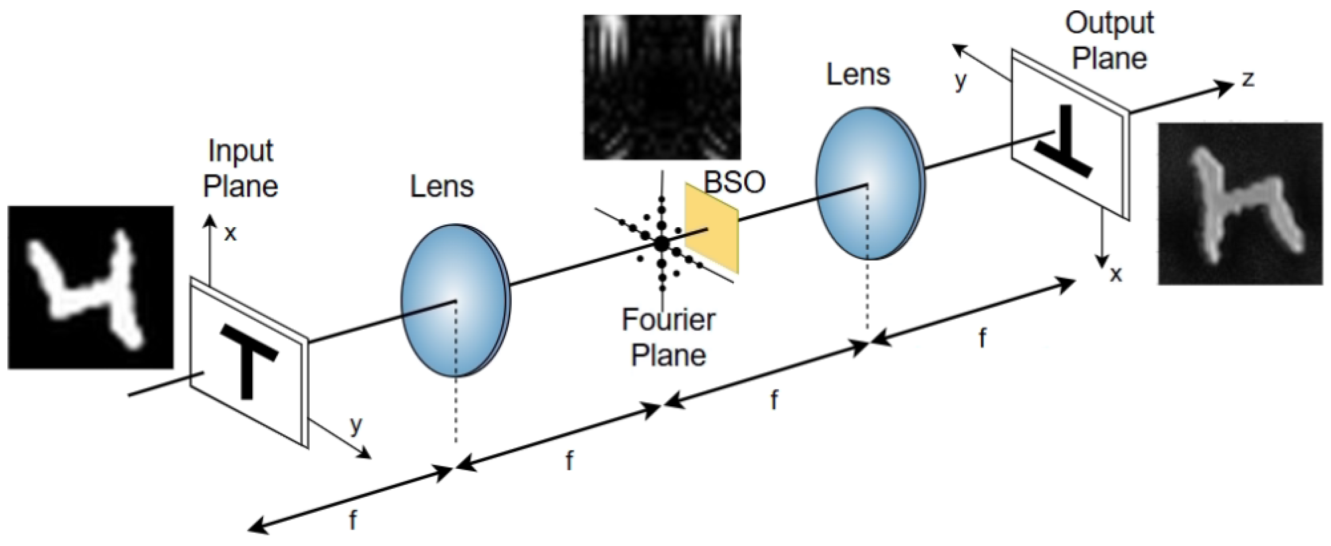
As shown in Figure 1, the optical convolution operation between the input image and the filter image is achieved using a 4f optical system. Initially, the input plane containing the input image is illuminated and passed through the first lens, which performs a Fourier transformation. In the Fourier domain, a filter or mask representing the convolution kernel is placed at the Fourier plane to modulate the transformed image’s spatial frequencies. The result of point wise multiplication of input image and kernel is then passed through a second lens, performing an inverse Fourier transform to produce the convolved image at the output plane. Figure 1 illustrates the process with representative images at each stage. Another fundamental component of digital CNNs is the nonlinear activation function. In our proposed approach, our aim is to implement this nonlinearity in the optical domain by incorporating photorefractive materials into the network, thereby enhancing the network’s ability to process intricate patterns and data relationships. The following section provides a detailed explanation of the all-optical nonlinear activation mechanism.

2.2. Optical Non-Linear Function

Deep neural networks require nonlinear activation functions to extract higher-order features. In digital CNNs, this nonlinearity is applied pointwise (e.g., ReLU, sigmoid) [14]. Without a nonlinear activation, the stacking layers collapse to a single linear transform. Achieving all-optical nonlinearity is challenging because most optical components are intrinsically linear at low power, and practical nonlinear materials are limited [15]. In our system, nonlinear activation is obtained from the intensity-dependent photorefractive phase response of a bismuth silicon oxide (BSO) crystal. Under illumination, photoionization and charge transport create a space-charge field that saturates with intensity. Under an applied bias, this behavior is modeled as $E_{sc}(x,y)=E_0/(1+I(x,y)/I_d)$, where $E_0$ is the applied electric field and $I_d$ is the dark-irradiance scale. Through the linear electro-optic effect, this field induces an index change and therefore a phase shift $\varphi (x,y)=k\Delta nL=-{\displaystyle \frac{1}{2}}k{n}^3{r}_{41}L{E}_{sc}(x,y)$, where $k=2\pi /\lambda$, n is the refractive index, $r_{41}$ is the electro-optic coefficient, and L is the crystal thickness. The BSO therefore acts as a phase-only nonlinear element, with $U_{out}(x,y)=U_{in}(x,y)exp\left[i\varphi (x,y)\right]$. At visible wavelengths in our operating regime, BSO is well approximated as nearly lossless: the field amplitude $\left|U\right|$ and total power are conserved, and any measured power variation arises from spatial redistribution rather than absorption [22]. To convert this phase nonlinearity into an effective intensity-dependent transmission suitable for an activation function, we use phase-to-amplitude conversion by spatial filtering. Specifically, the BSO crystal is placed near the Fourier plane of the 4f correlator, immediately after the kernel SLM, and a finite circular iris is introduced in the subsequent image plane. The intensity-dependent BSO phase reshapes the diffraction pattern, and the iris clips the redistributed field. As a result, the collected output power becomes a nonlinear function of the input intensity. The main BSO crystal parameters used for nonlinear activation are summarized in

Table 2. Main BSO crystal parameters used for the nonlinear activation.

Parameter	Value
Material	Bismuth silicon oxide (BSO)
Crystal size	$12\mathrm{mm}\times 12\mathrm{mm}\times 5\mathrm{mm}$
Crystal orientation	[110] ± 2%
Surface quality	40/20 scratch-dig
Clear aperture	>$85\%$
Coating	AR at 632.8 nm

.

In the simulation model, the BSO response was described using $n=2.54$, $r_{41}=5.0\times {10}^{-12}\mathrm{m}/\mathrm{V}$, $E_0=2.0\times {10}^6\mathrm{V}/\mathrm{m}$, and $I_d=120\mathrm{W}/{\mathrm{m}}^2$ at 632.8 nm.

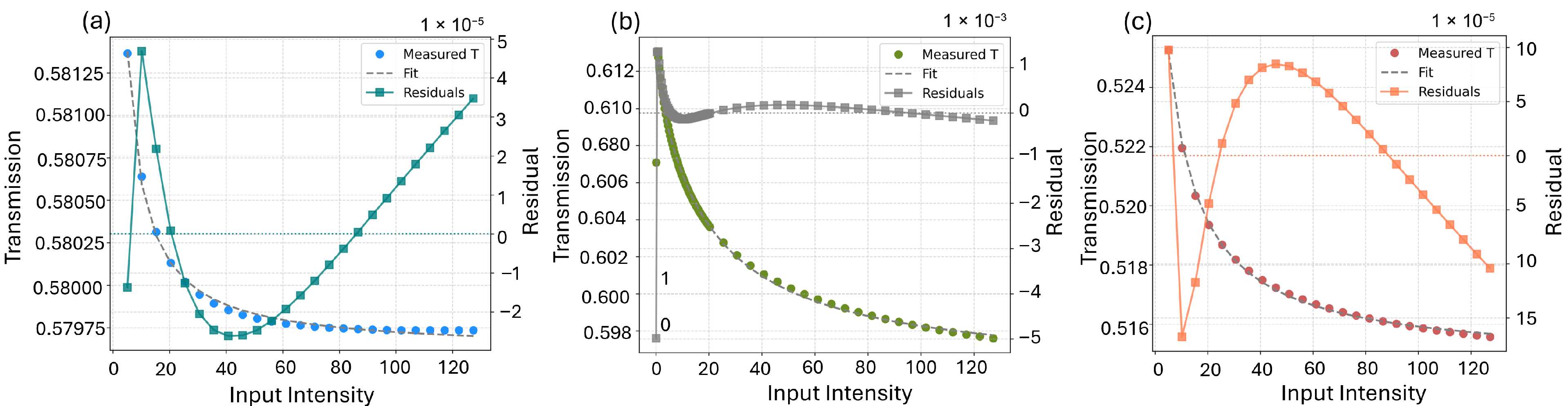
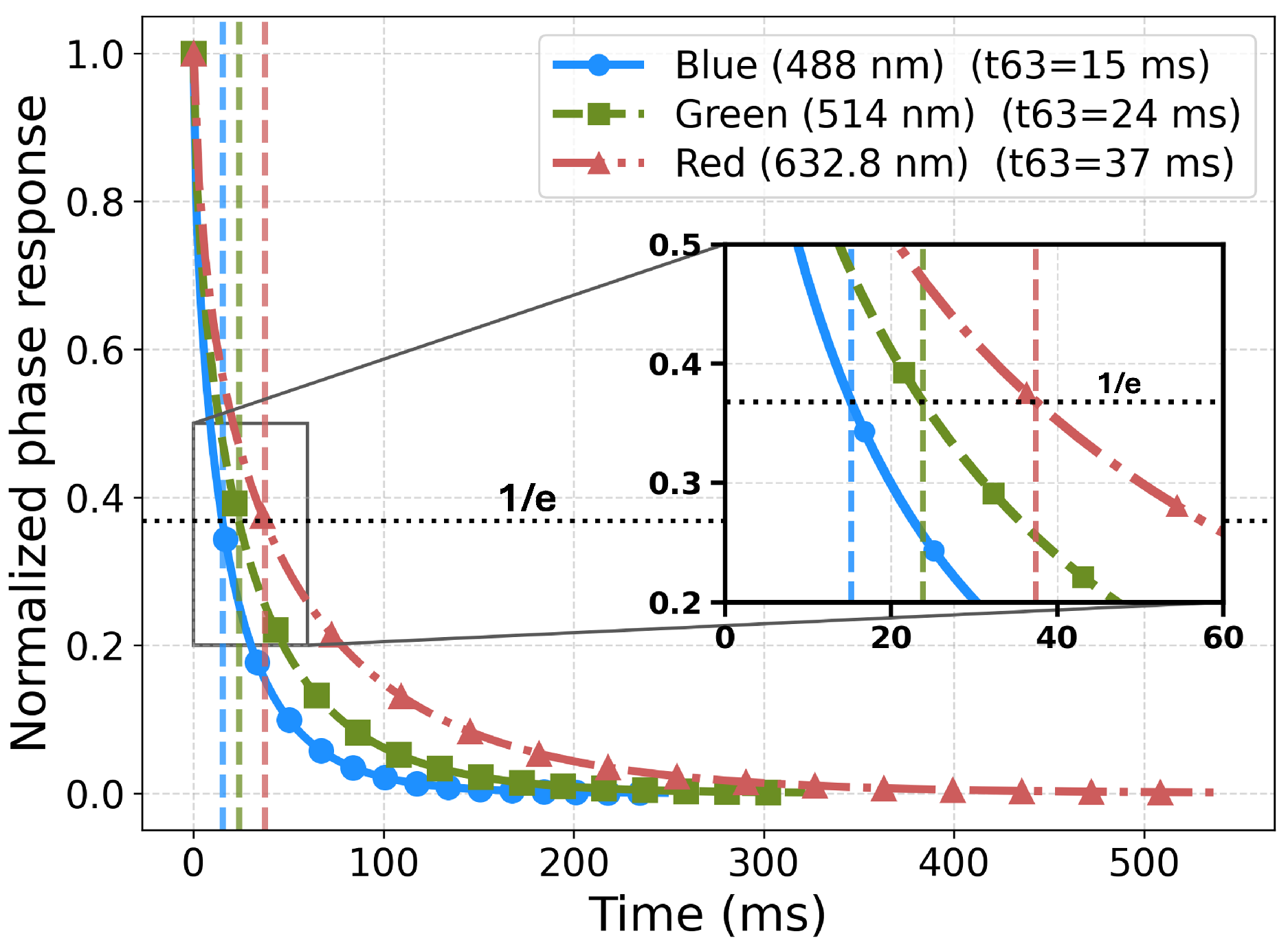
The measured transmission is defined as $T=P_{out}/P_{in}$, where $P_{out}$ is measured after the iris. Importantly, this $T\left(I\right)$ describes a system-level nonlinearity, namely the combination of BSO phase modulation and aperture filtering, rather than intrinsic absorption in the BSO crystal. If the iris is fully open or removed, the transformation is approximately unitary and $P_{out}\approx P_{in}$, nearly independent of intensity. For compact characterization, the transmission is fitted using the saturating model $T\left(I\right)=T_{min}+(T_{max}-T_{min})I/(I+I_0)$, where $I_0$ captures the effective photorefractive intensity scale. Figure 2 shows $T\left(I\right)$ at 488, 514, and 632.8 nm for the 5 mm BSO crystal. The curvature is strongest at shorter wavelengths, consistent with higher photorefractive sensitivity [23,24]. We also quantify the temporal dynamics of phase buildup. The evolution of the space-charge field is modeled as a first-order process, $E_{sc}\left(t\right)=E_{sc}^{\infty }+(E_0-E_{sc}^{\infty })exp[-t/\tau \left(I\right)]$, with $\tau \left(I\right)={\tau }_{\mathrm{dark}}/(1+I/I_d)$. We report $t_{63}$, defined as the time required to reach 63% of the final phase response, corresponding to $(1-1/e)$.

Figure 3 shows the normalized temporal phase response of the BSO crystal at representative visible wavelengths. The extracted $t_{63}$ response times are 15 ms at 488 nm, 24 ms at 514 nm, and 37 ms at 632.8 nm, where $t_{63}$ is the time required to reach 63% of the final phase response. Since the OCNN simulations are performed at 632.8 nm, the relevant BSO settling time is approximately $37\mathrm{ms}$. This corresponds to a 63%-settling update rate of approximately $1/t_{63}\approx 27\mathrm{Hz}$. If the BSO response is approximated as a first-order process, the equivalent small-signal 3-dB bandwidth is $1/\left(2\pi t_{63}\right)\approx 4.3\mathrm{Hz}$. The additional latency and resource cost introduced by the BSO nonlinear activation are summarized in

Table 3. Additional latency and resource cost introduced by the BSO nonlinear activation.

Parameter	Linear OCNN	BSO-Based OCNN
Nonlinear element	None	BSO crystal + iris
latency	SLMs	SLMs + BSO response
$t_{63}$ at 632.8 nm	–	≈37 ms
Approx. BSO bandwidth	–	≈4.3 Hz

. In the present optical engine, the BSO settling time is not the main bottleneck because it is comparable to the update time of the SLMs used in the system. However, for future systems using faster modulators and detectors, the BSO response may become the dominant bandwidth limitation. This response time can be improved by optimizing the operating wavelength, optical intensity, bias field, crystal thickness, and controlled heating conditions.

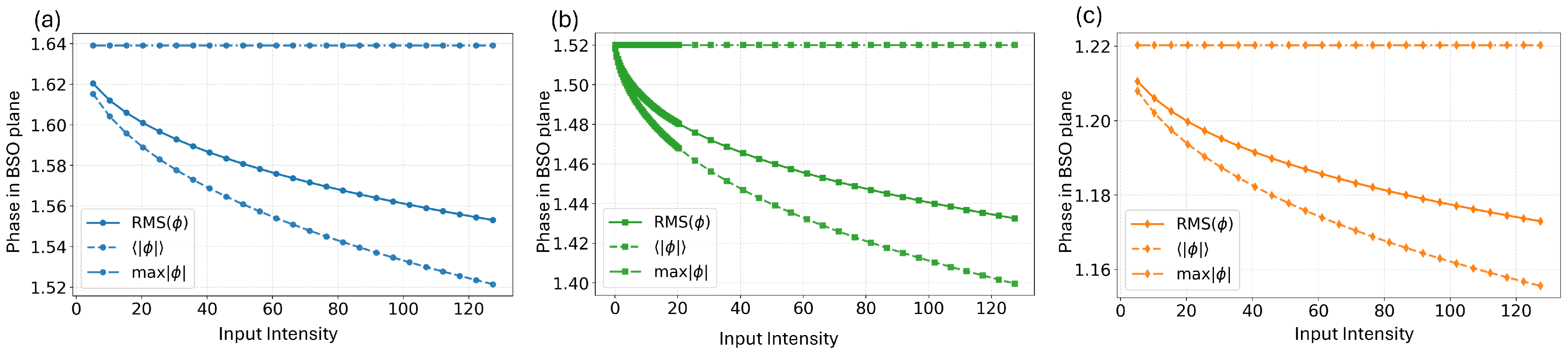
To directly connect the observed transmission nonlinearity with the underlying phase response, Figure 4 reports the BSO-plane phase metrics, including RMS $\varphi$, mean $\left|\varphi \right|$, and maximum $\left|\varphi \right|$, as functions of input intensity. Together, Figure 2, Figure 3 and Figure 4 show that the BSO element provides an intensity-dependent phase response and that, when combined with a finite iris, this phase modulation is converted into an effective amplitude nonlinearity.

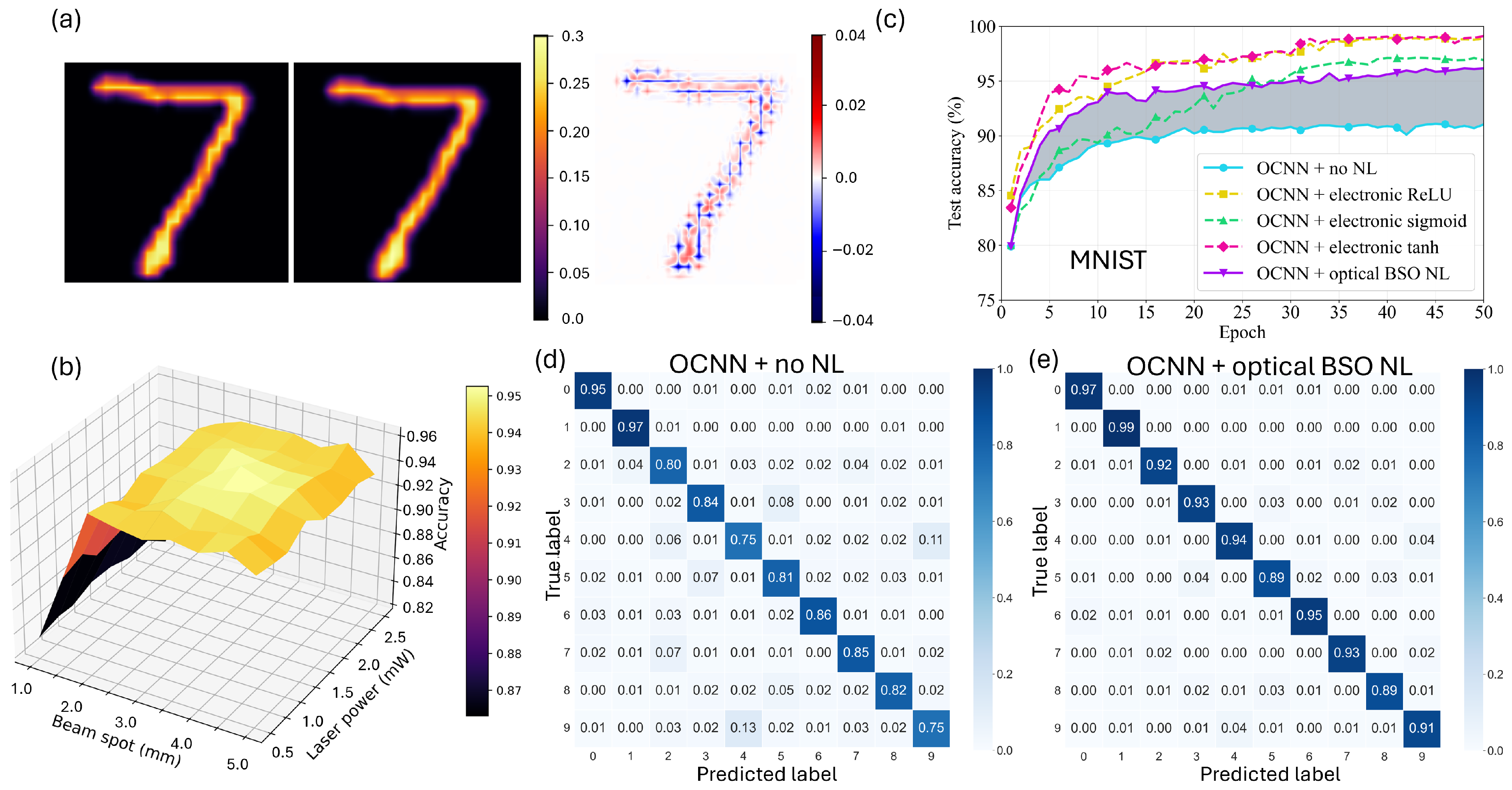
To quantify the role of optical nonlinearity in classification, we compared two OCNNs on MNIST: a linear OCNN and the proposed BSO-based nonlinear OCNN. The nonlinear model produces sharper and higher-contrast feature maps, as shown in Figure 5a, which improves class separability for the following classifier.

To further compare the proposed optical nonlinearity with conventional electronic nonlinear activation functions, we evaluated five cases under the same optical convolution front-end and training protocol: an OCNN without nonlinear activation, OCNN with electronic ReLU, OCNN with electronic sigmoid, OCNN with electronic tanh, and OCNN with the proposed optical BSO nonlinearity. The electronic nonlinearities provide the highest classification accuracy, with ReLU and tanh reaching final test accuracies of 97.65% and 97.80%, respectively. The proposed BSO nonlinearity reaches a lower final accuracy of 95.05% and a best test accuracy of 95.70%, but still clearly improves performance compared with the OCNN without nonlinear activation, which reaches 90.85%. Therefore, the purpose of the BSO layer is not to outperform ideal electronic activations but to demonstrate a physically implemented optical nonlinear transformation that reduces dependence on electronic post-processing and supports progress toward more fully optical neural-network architectures.

Both the linear and BSO-based OCNNs were trained end-to-end for 35 epochs using the same training protocol. A sweep of the BSO beam-spot radius and input optical power reveals a clear optimum operating region, as shown in Figure 5b. Outside this region, the classification accuracy decreases because insufficient illumination weakens the photorefractive response, whereas excessive optical power drives the BSO response toward saturation. The test curves in Figure 5c show test accuracy versus epoch for the same optical CNN with different non linear functions. The BSO-based OCNN converges faster and reaches a lower loss than the linear OCNN baseline. At the optimum operating point of $P=1.67\mathrm{mW}$ and $r_{\mathrm{rms}}=3.5\mathrm{mm}$, the BSO-based OCNN achieves a final test accuracy of 95.7%, compared with 90.8% for the linear OCNN. This improvement is also reflected in the confusion matrices in Figure 5d,e show the confusion matrices for optical CNN without non linear function and optical CNN with optical non linear function, respectively. In the linear OCNN, the cascaded 4f convolution, propagation, aperture, and readout stages remain approximately linear before the electronic classifier. This limits the separability of classes whose optical features overlap after convolution. In contrast, the BSO crystal introduces an intensity-dependent photorefractive phase shift, and the following iris converts the resulting phase redistribution into an effective amplitude nonlinearity.

Therefore, weak, intermediate, and strong spatial-frequency components are not transmitted with the same linear scaling. This nonlinear redistribution produces sharper and more discriminative optical feature maps, increases inter-class separability, and reduces the dependence of the classifier on purely linear intensity scaling.

Unlike a digital ReLU, which applies an electronic pointwise threshold after numerical convolution, the proposed BSO activation performs a physical intensity-dependent phase modulation followed by iris-based phase-to-amplitude conversion. Therefore, the most direct ablation is the comparison between the same optical system with and without the BSO response, as presented in Figure 5.

2.3. Optical Pooling Layer

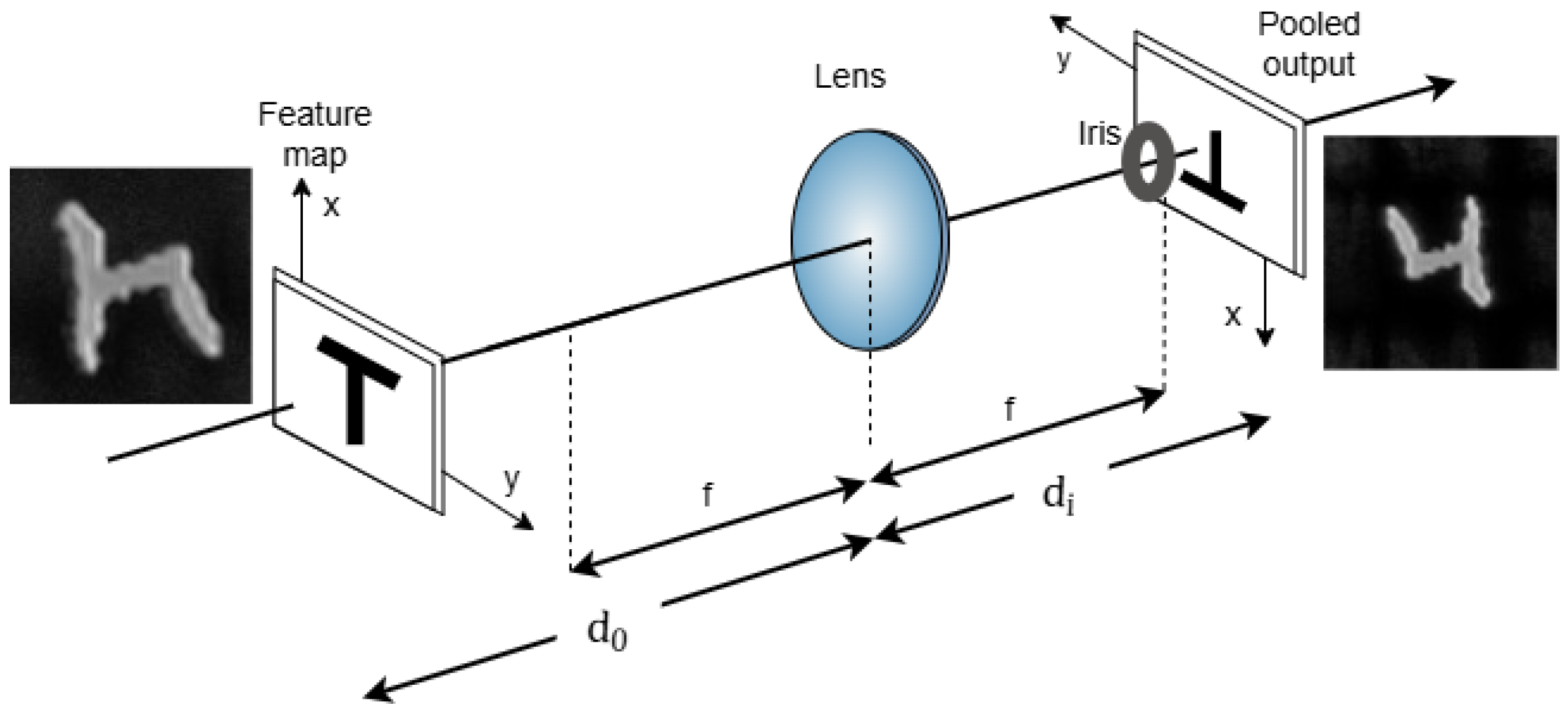
The pooling is a standard operation in convolutional neural networks used to reduce the spatial dimensionality of feature maps, reducing the number of parameters and the computational burden of subsequent layers while improving the robustness to small spatial variations [25]. In digital CNNs, pooling is typically implemented through local operators, such as average pooling or maximum pooling [15]. We implement an all-optical pooling layer that is functionally analogous to average pooling, realized as spatial-frequency low-pass filtering followed by down-sampling (anti-aliased pooling). Our pooling stage consists of a single convex lens that images the input feature map onto a reduced-size output plane. The feature map is placed at a distance $d_o$ from the pooling lens, and the pooled image is formed at a distance $d_i$. Under the thin-lens and paraxial approximations, the imaging geometry is governed by ${\displaystyle \frac{1}{f}}={\displaystyle \frac{1}{d_o}}+{\displaystyle \frac{1}{d_i}}$ and $M={\displaystyle \frac{h_i}{h_o}}=-{\displaystyle \frac{d_i}{d_o}}$, where f is the focal length of the pooling lens, M is the magnification, and $h_o$ and $h_i$ are the heights of the object and the image, respectively. By operating in the demagnification regime $\left|M\right|<1$, the lens performs optical downsampling by compressing the spatial extent of the feature map. To explicitly enforce anti-aliasing prior to down-sampling, we place a circular aperture stop (iris) at the back focal plane of the pooling lens. This iris limits the transmitted spatial-frequency bandwidth, implementing a tunable low-pass filter that removes high spatial frequencies that would otherwise be aliased after demagnification and sampling. The subsequent demagnified imaging onto the detector then performs the down-sampling. Together, aperture stop and demagnification realize a low-pass and down-sample operation that is directly analogous to average pooling in digital CNNs.

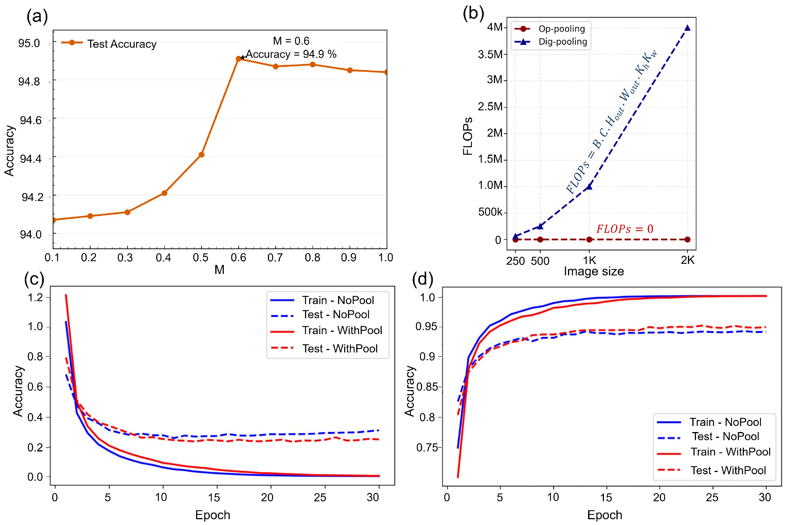
Figure 6 illustrates the optical pooling configuration and representative feature maps before and after pooling. The pooling strength is continuously controlled by the magnification M, which can be tuned by adjusting $d_o$ and $d_i$ while satisfying the lens equation. To evaluate the impact of optical pooling on classification performance, we swept M and measured MNIST test accuracy (Figure 7a). The highest test accuracy 94.9% occurs at $M=0.6$, indicating an optimal tradeoff between preserving discriminative spatial detail and reducing spatial resolution. Although pooling does not significantly increase peak accuracy for MNIST, it improves generalization trends consistent with the role of pooling in conventional CNNs (Figure 7c,d) [26].

Finally, this pooling operation is performed entirely in the optical domain without intermediate digital computation. Unlike digital average pooling, whose operation count scales with feature-map size, the optical pooling layer introduces no additional digital FLOPs during inference, since the low-pass filtering and down-sampling are realized by passive propagation through a lens and Fourier-plane aperture (Figure 7b).

3. Noise in Optical CNN: Theory and Analysis

Real free-space optical processors deviate from ideal, noise-free simulations because of source instabilities, aberrations, misalignment, dust contamination, and other hardware imperfections. During inference, these physical noises can distort the optical feature maps produced by the 4f correlator and reduce the classification accuracy. In this section, we introduce a physically interpretable noise model for the proposed OCNN, quantify the effect of each noise mechanism, and evaluate the sensitivity of the network to different aberration.

We model the dominant degradations expected at the camera intensity plane of a free-space optical implementation. We let $h(x,y)$ denote the input image displayed on the input SLM, $g(x,y)$ denote the learned convolution kernel implemented in the Fourier plane, and $I_0(x,y)$ denote the camera-plane intensity feature map. In the ideal case, the 4f processor implements Fourier-domain filtering, and the nominal feature map can be written in the intensity-domain model as $I_0(x,y)=h(x,y)\otimes g(x,y)$, where $\otimes$ denotes convolution. We consider four physical noise mechanisms: laser power fluctuation, wavefront aberration, misalignment, and dust. Laser fluctuation is modeled as a multiplicative noise, $I_1(x,y)=(1+n_1)I_0(x,y)$, where $n_1$ represents relative intensity noise and is sampled as a zero-mean fluctuation. Wavefront aberration is modeled using a pupil-plane phase error, $P_{\mathrm{ab}}(\rho ,\theta )=P(\rho ,\theta )exp[i2\pi W(\rho ,\theta )/\lambda ]$, where $P(\rho ,\theta )$ is the circular pupil function and $W(\rho ,\theta )$ is the wavefront error. In the normalized noise comparison, spherical aberration is used as the representative wavefront-aberration case because the Zernike sensitivity analysis below shows that it is the most damaging mode.

Misalignment is modeled as a subpixel zero-padded shift of the camera-plane intensity, $I_3(x,y)=I_2(x-\Delta x,y-\Delta y)$, where $(\Delta x,\Delta y)$ represents lateral displacement between the optical feature map and the detector sampling grid. Dust contamination is modeled as a multiplicative attenuation mask, $I_{\mathrm{out}}(x,y)=I_3(x,y)m_{\mathrm{dust}}(x,y)$, where $m_{\mathrm{dust}}\in [0,1]$ is fixed in the sensor coordinates. Fully opaque particles correspond to $m_{\mathrm{dust}}=0$ inside the particle footprint, while partial opacity gives $0<m_{\mathrm{dust}}<1$.

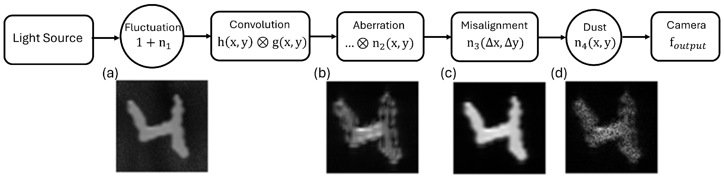
This intensity-domain model is a compact system-level approximation of the full coherent wave-optics perturbation process. It is designed to reproduce the dominant detector-plane signatures and to enable controlled robustness studies. Figure 8 summarizes the noise injection pathway and illustrates the characteristic effect of each mechanism on the feature map. Laser fluctuation changes the overall intensity level (Figure 8a), wavefront aberration redistributes the optical field (Figure 8b), misalignment shifts the feature map relative to the classifier sampling grid (Figure 8c), and dust introduces localized attenuation (Figure 8d).

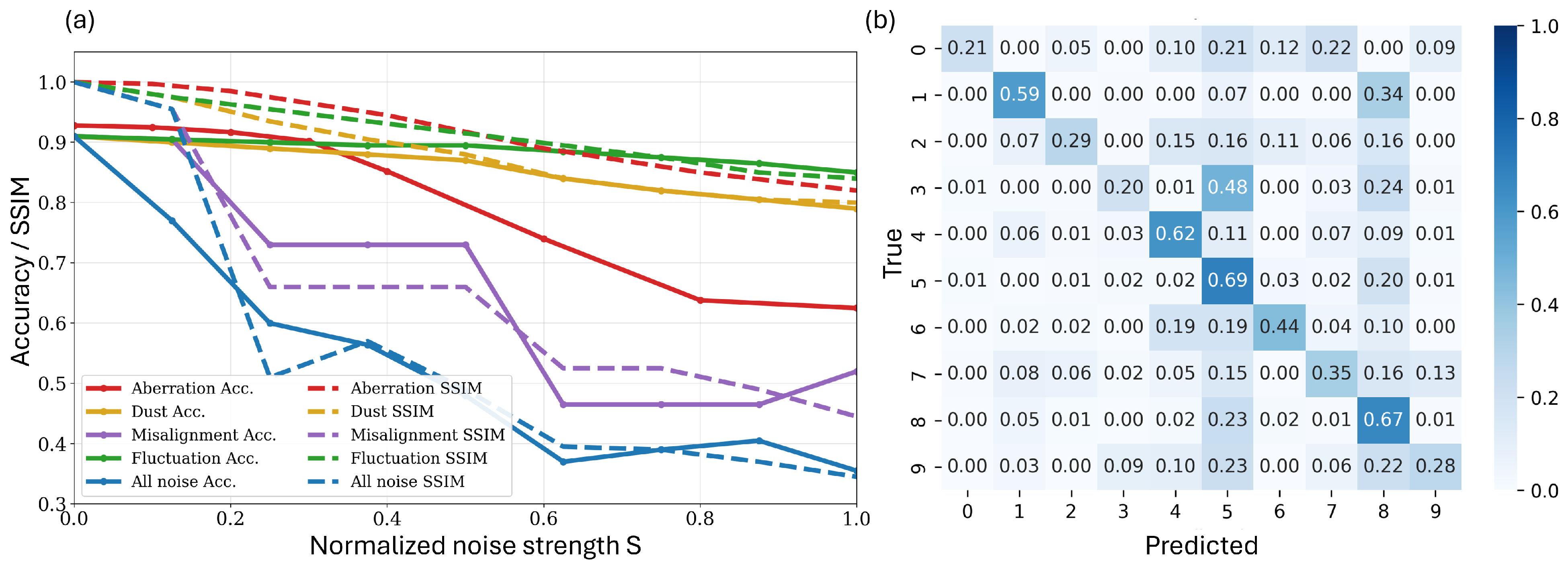
To quantify robustness, the network was first trained end-to-end under clean conditions, and the physical noise sources were then injected only during inference. We evaluated both classification accuracy and feature-map fidelity. Feature-map fidelity was quantified using the Structural Similarity Index Measure (SSIM), which compares luminance, contrast, and structural similarity between the clean and degraded optical feature maps. Because the native parameters of the noise sources have different physical units, direct comparison using their raw values is not meaningful. Therefore, each perturbation was evaluated using a normalized strength parameter $s\in [0,1]$, where $s=0$ corresponds to the clean condition and $s=1$ corresponds to the maximum tested strength for that perturbation. For spherical aberration [27], the normalized strength corresponds to the RMS wavefront-error sweep, with $s=1$ equivalent to $0.5\lambda$. For other noise sources, the native parameter $\theta$ was swept and the SSIM between the clean feature map and the degraded feature map was computed. A reference value ${\theta }^{*}$ was then defined at a common reachable degradation level, $\mathrm{SSIM}\left({\theta }^{*}\right)=0.73$, which was the lowest SSIM level reached by all considered noise mechanisms over the tested parameter ranges. The normalized noise strength was defined as $s={\displaystyle \frac{1-\mathrm{SSIM}\left(\theta \right)}{1-\mathrm{SSIM}\left({\theta }^{*}\right)}}$. Figure 9a shows the test accuracy and mean SSIM versus normalized noise strength s. Solid curves represent classification accuracy, while dashed curves represent mean SSIM. Laser fluctuation has the weakest influence on accuracy because it mainly changes the overall optical intensity while largely preserving spatial structure.

Dust and spherical aberration produce stronger degradation because they remove or redistribute local spatial information in the optical feature map. Misalignment causes moderate degradation as the shifted feature map becomes increasingly mismatched with the classifier sampling grid. When all noise sources are applied simultaneously at the same normalized strength, the performance degradation is stronger than for any individual noise source, confirming the compounding effect of realistic optical perturbations. Figure 9b shows the normalized confusion matrix for the all-noise condition at $s=0.9$. This operating point represents a severe but calibrated degradation level, where spherical aberration, dust, detector misalignment, and laser fluctuation are applied using their SSIM-calibrated native parameters. The normalized noise-comparison analysis uses spherical aberration as a representative wavefront-error case. However, wavefront sensitivity is generally mode-dependent; therefore, we also performed a separate Zernike-aberration analysis. The aberrated pupil was modeled as $P_{\mathrm{ab}}(\rho ,\theta )=P(\rho ,\theta )exp[i2\pi W(\rho ,\theta )/\lambda ]$, where $W(\rho ,\theta )=a_j{Z}_j(\rho ,\theta )$ is the wavefront error represented by a normalized Zernike mode. The RMS wavefront-error amplitude was swept from 0 to $0.5\lambda$ for defocus, astigmatism, coma, and spherical aberration.

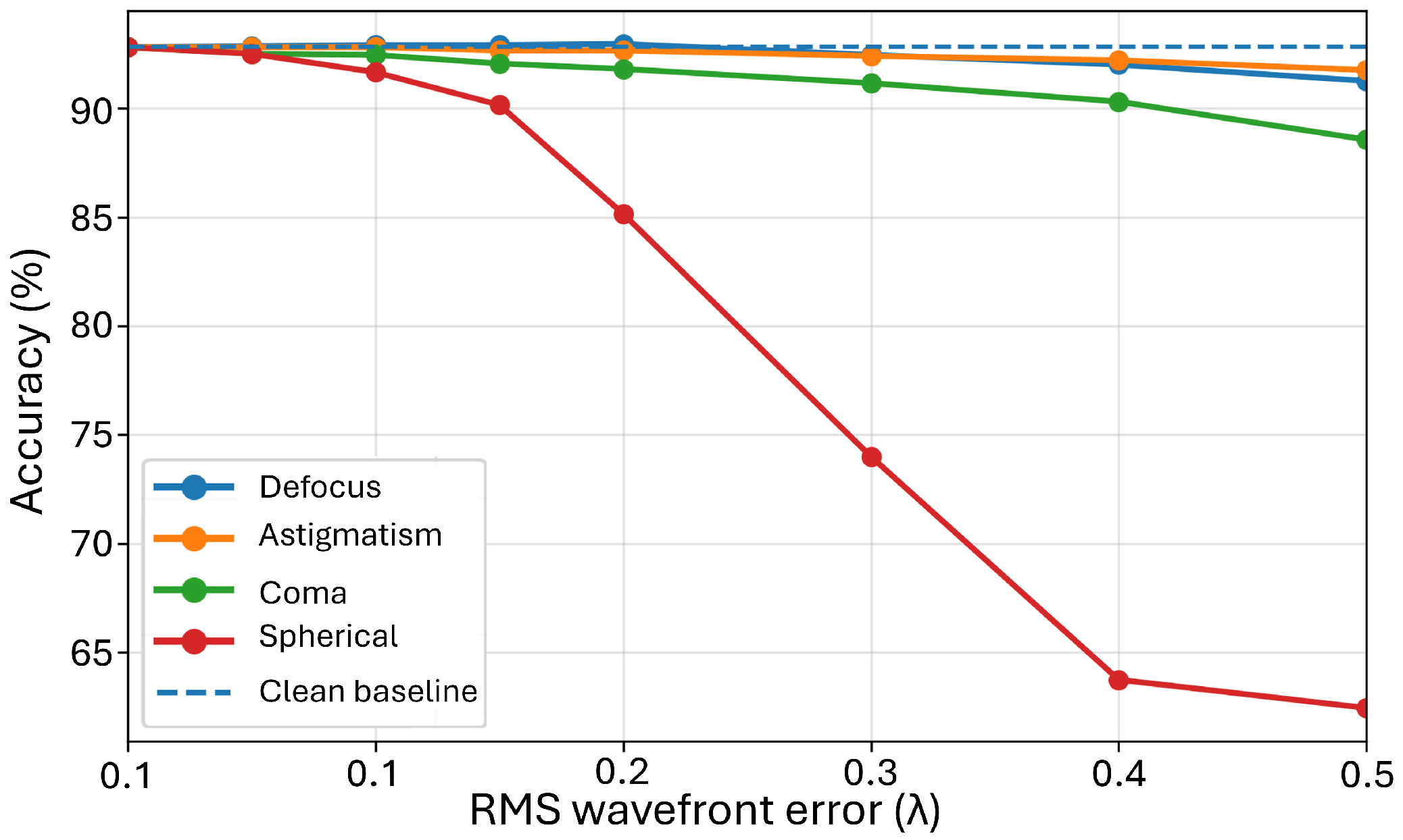
Figure 10 shows the resulting test accuracy as a function of RMS wavefront error. The OCNN is relatively robust to defocus, astigmatism, and coma over the studied range, with only a moderate accuracy reduction up to $0.5\lambda$. In contrast, spherical aberration produces the strongest degradation, reducing the test accuracy from the clean baseline to approximately 65% at $0.5\lambda$. These results show that a defocus-only model underestimates the effect of higher-order wavefront distortions and that robustness depends strongly on the aberration mode. Together, these results show that realistic optical noise reduces both feature-map fidelity and classification accuracy in a mechanism-dependent manner. The analysis motivates two complementary strategies for robust optical CNNs: careful optical tuning to reduce wavefront aberrations, detector misalignment, and contamination, and noise-aware training so that the classifier adapts to expected physical variability. In the next section, we build on this foundation to introduce a loop-based deep OCNN architecture that implements multiple optical convolutions, optical nonlinear activation, and pooling operations efficiently.

4. Loop-Based DOCNN and Performance Evaluation

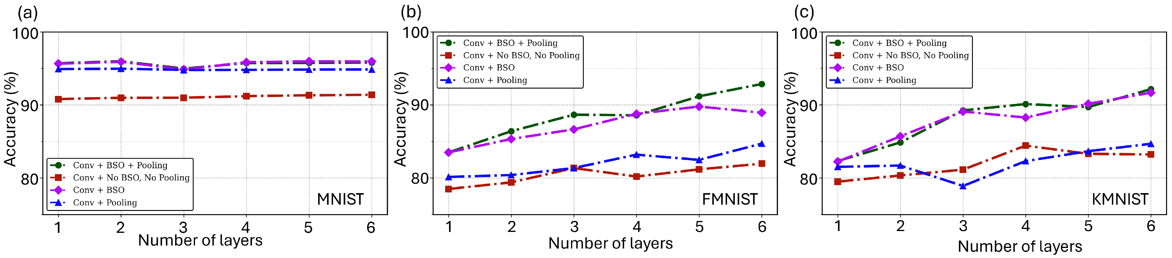
Deep convolutional neural networks (DCNNs) achieve strong performance in vision tasks by stacking multiple layers to build hierarchical feature representations, progressing from edges and textures to more abstract structures. In conventional electronic hardware, however, the computational and memory cost of repeated convolutions grows rapidly with depth, increasing latency, and power consumption. To address this bottleneck in free-space optical inference, we propose a loop-based deep optical CNN (DOCNN) that achieves depth by reusing a single optical processing block across multiple passes, rather than physically cascading many distinct optical layers. The DOCNN is built around one reconfigurable 4f correlator that implements a learned convolutional operation, followed by the optical nonlinearity and the optical pooling stage. To extend the optical correlator from a single convolutional layer to multiple subsequent layers, we iteratively record the output of each convolutional layer $\left(t\right)$, denoted as $ou{t}_t$, and use it as input for the next layer, so that $i{n}_{(t+1)}=ou{t}_t$. Repeating this procedure for N passes produces an $N-layer$ DOCNN while reusing the same fixed optical hardware. After the final pass, the measured intensity is converted to a tensor, normalized, and fed to a lightweight two-layer fully connected classifier in the electronic domain. To investigate the contribution of individual optical components in a deep OCNN, we conducted the performance evaluation in four architectural forms: (1) $4f$ convolutional stages without nonlinearity or pooling, (2) $4f$ convolutional stages with only optical nonlinearities, (3) 4f convolutional stages with only optical pooling layer, and (4) 4f convolutional stages with photorefractive nonlinearities and optical pooling layer. Each configuration was tested with network depths ranging from one to six layers for different dataset (MNIST, FMNIST, KMNIST). Figure 11 shows the classification accuracy of different architectures in different datasets. In general, the accuracy tends to improve as the depth of the network increases, highlighting the importance of deep feature hierarchies. However, the effect of depth varies across datasets. For the MNIST dataset (Figure 11a), increasing the number of layers leads to only marginal improvement, likely because the dataset is relatively simple and does not require deeper representations. In contrast, for the more complex FMNIST and KMNIST datasets, accuracy improves more noticeably with greater depth. This suggests that deeper layers are able to extract more informative and discriminative features, which enhances classification performance. As illustrated in Figure 11, the blue curves show that, in all datasets, the pooling does not significantly improve classification accuracy. However, incorporating a pooling layer remains essential to reduce the dimensionality of the image. Furthermore, the pooling operation is performed entirely in the optical domain, eliminating the need for intermediate digital computation.

The best results are achieved with the full configuration, 4f convolutional stages, BSO nonlinearities, and optical pooling stage, which consistently outperformed the other variants at all depths (Figure 11).

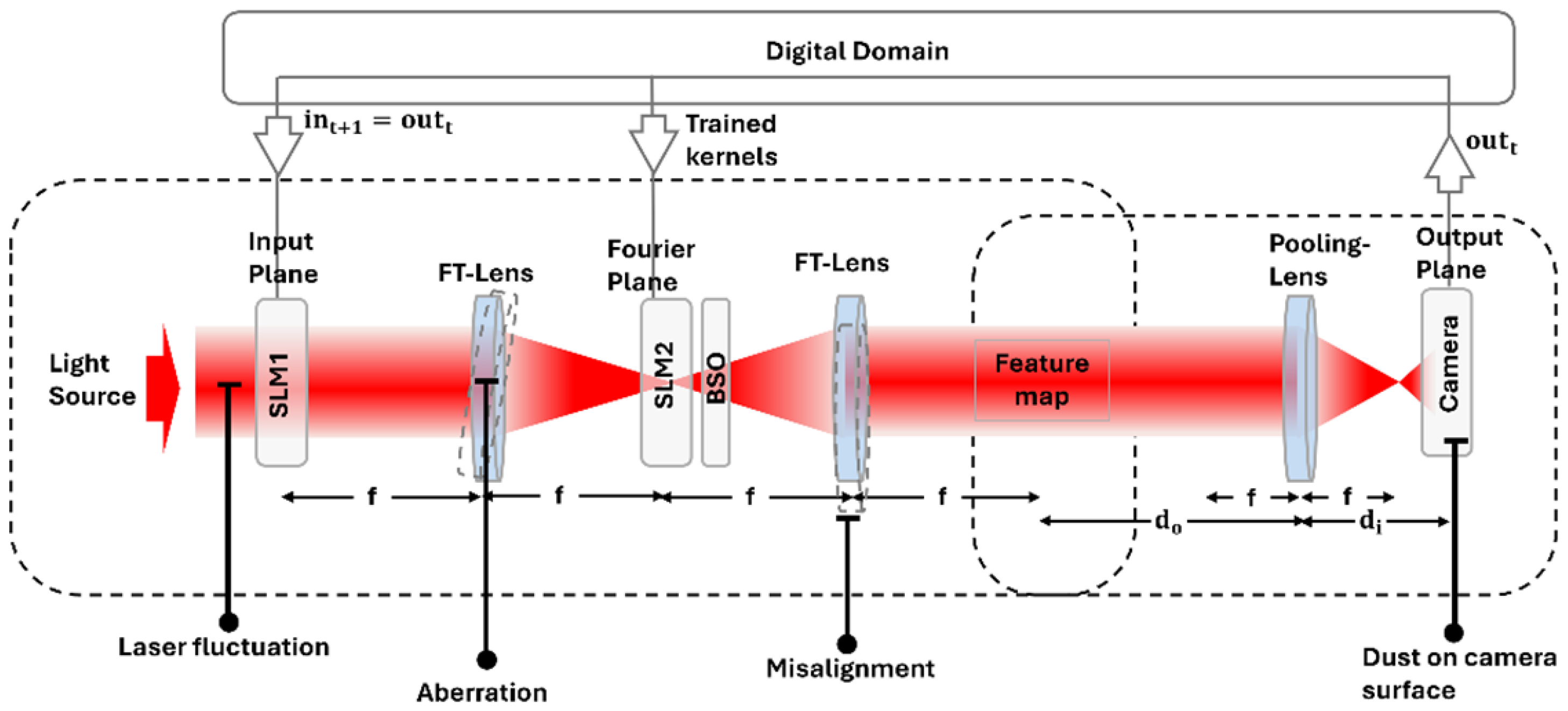
Because free-space optical systems are unavoidably exposed to physical perturbations, we next quantify the impact of realistic noise on loop-based DOCNN performance. We train the network end-to-end under clean (noiseless) conditions and inject noise only during inference using the same four mechanisms introduced in Section 3: laser power fluctuation, blur/aberration, misalignment, and dust/occlusion. Figure 12 summarizes the loop-based optical path and indicates where each noise source acts. Compared to physically stacking many optical layers, the loop-based approach is expected to reduce the number of unique optical elements that must be aligned and calibrated, which simplifies mechanical alignment and supports stable operation.

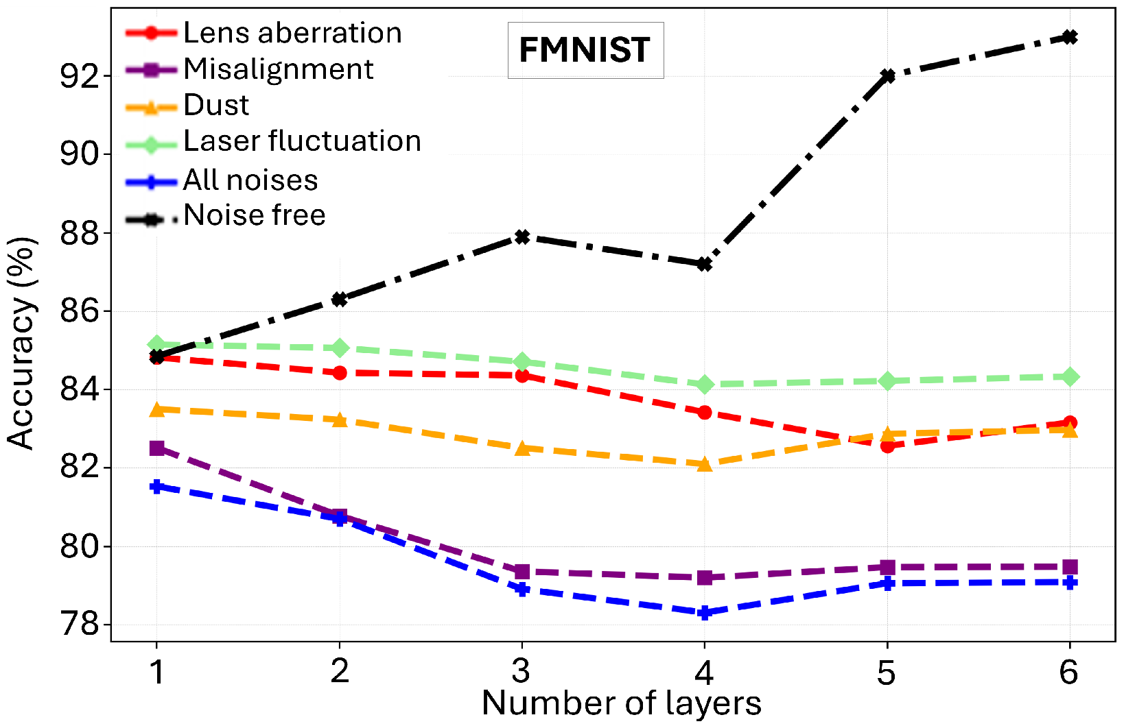
To compare noise sources with different native units on the same footing, we use the SSIM-based normalized severity s defined in Section 3, selecting each noise parameter to match the same normalized strength. Figure 13 shows the test accuracy versus depth for FMNIST under fixed s for each noise mechanism. Under equalized severity, increasing depth yields only modest accuracy improvements in noisy conditions, indicating that physical noise can limit the benefit of deeper optical processing when the model is trained only on clean data.

Together, these results show that loop-based depth provides a compact route to deep optical CNNs, but realistic physical noise still limits performance, motivating the noise-aware training strategy developed in the next section.

5. Noise-Aware Training and Performance Improvement

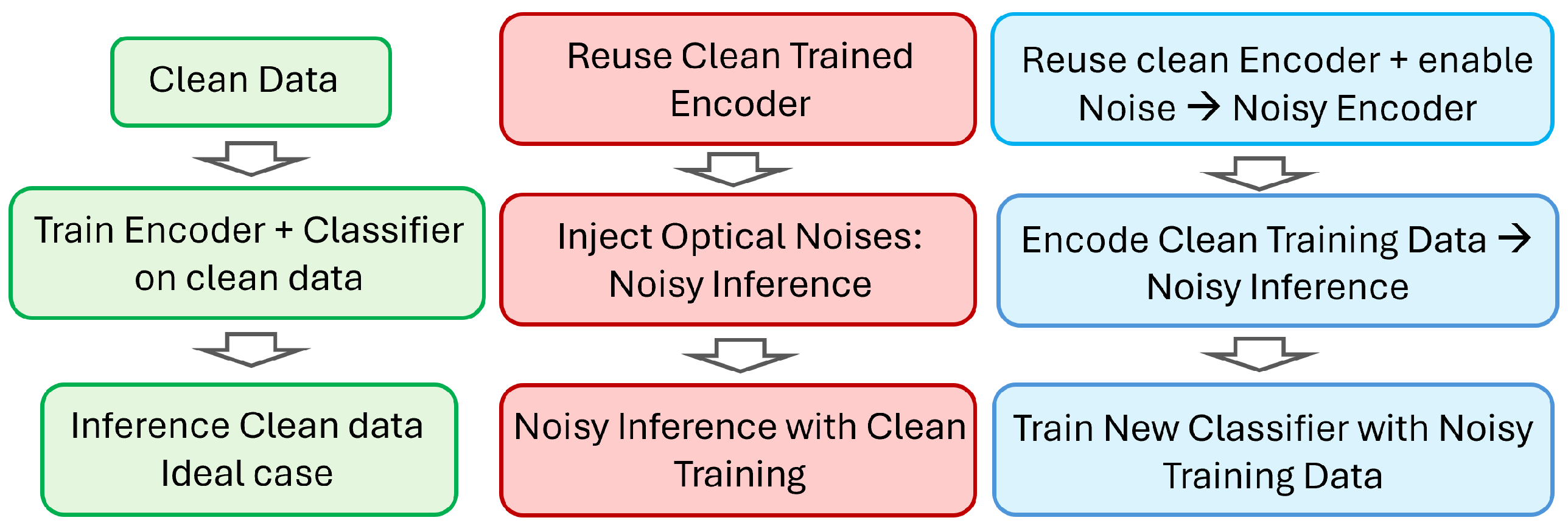
Models trained only on clean, noise-free data often perform well under ideal conditions but degrade when deployed under realistic noise [28,29]. In free-space optical inference, such noises arise from system-level effects including lens aberrations, intensity fluctuations, misalignments, dust, etc. Without considering these effects during training, the network tends to overfit idealized patterns and creates a training-test domain gap that reduces the precision of inference [30]. To mitigate this gap without requiring complete end-to-end retraining of the optical encoder, we adopt a feature-level noise-aware training strategy [31]. In general, noise injection during training acts as a regularizer and can improve robustness and generalization under distribution changes [32]. Noise-aware training can be implemented in several ways depending on where the noise is introduced. A common approach is data-level augmentation, where noise is added directly to the input examples (e.g., Gaussian perturbations, blur, or occlusions), forcing the model to learn representations that remain stable under such distortions [29]. Feature-level noise injection, which we adopt here, perturbs the intermediate representations rather than the input. This can be implemented by injecting noise directly into feature maps or, equivalently, by passing clean data through a noisy encoder to generate corrupted feature embeddings [33,34]. Alternative robustness strategies exist, but are less aligned with our experimental constraints. Model-level approaches inject noise into internal computations or parameters (e.g., weight noise), which can improve stability but do not directly reflect hardware-specific distortions [35,36]. A more direct approach is hardware-in-the-loop or physics-aware training, where the physical device (or a differentiable simulator) is integrated into end-to-end optimization so that the model adapts to hardware-specific variability [37,38]. More generally, robustness can also be encouraged by modifying the loss to penalize sensitivity to perturbations, even when those perturbations are not explicitly observed during training [39,40]. In this work, we focus on feature-level noise-aware training because it is simple to implement in a loop-based DOCNN and provides a practical route to robustness without requiring repeated end-to-end retraining of the optical encoder. Among these approaches, our work focuses on feature-level noise injection, which is particularly suited to free-space optical neural networks. To evaluate the effectiveness of this approach, we compare three configurations: (i) clean training with clean inference (ideal case), (ii) clean training with noisy inference, and (iii) noise-aware training with noisy inference (proposed method). In the (i) configuration, both the encoder and classifier are trained and tested on noise-free data, establishing an ideal baseline. In the (ii) configuration, the same clean-trained encoder is reused, but inference is performed with the full noisy optical system activated, revealing the significant performance degradation that occurs when noise is not accounted for during training. In the (iii) proposed configuration, the noise-aware approach, the full clean training set is propagated through this noisy encoder once to generate noise-corrupted feature representations, and a new classifier is trained on these features while keeping the encoder weights fixed. This feature-level augmentation explicitly matches the classifier’s training distribution with the noisy feature distribution produced by the optical hardware, reducing the domain gap between training and inference.

Because the system learns from features that include realistic physical imperfections, it becomes more resistant to errors and better at detecting the difference between important information and unwanted variations. Being exposed to these imperfections helps the system correct itself, preventing it from simply memorizing perfect examples. Instead, it pushes the system to find stable representations that do not change easily when faced with disruptions. Figure 14 illustrates this training pipeline.

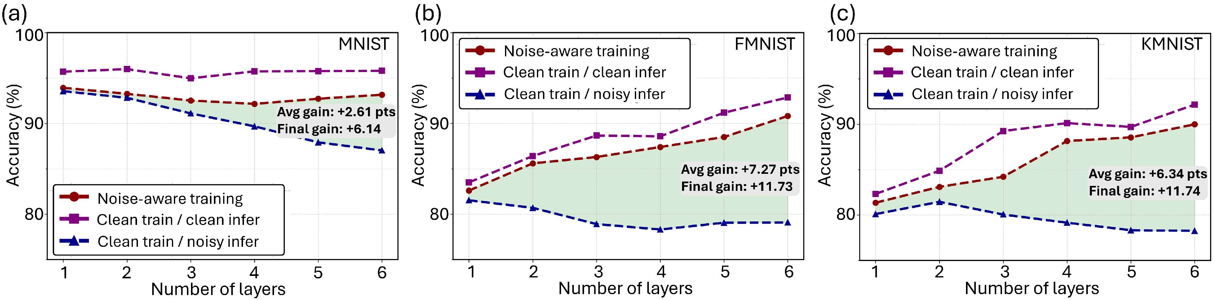
Figure 15 compares three different methods for loop-based DOCNN across number of layers on MNIST, FMNIST, and KMNIST: clean training with clean inference, clean training with noisy inference, and the proposed feature-level noise-aware training. In all three datasets, introducing optical noise only at inference causes a clear drop in accuracy relative to the clean inference baseline. Noise-aware training consistently recovers a substantial part of this loss. In MNIST, the degradation caused by noisy inference is relatively moderate, and noise-aware training yields a smaller but still consistent improvement, with an average gain of $2.61$ percentage points (pts) and a maximum gain of 6.14 pts at 6 layers. In contrast, for the more challenging datasets, FMNIST and KMNIST, the benefit of noise-aware training is much more pronounced. In both datasets, noisy inference causes a large drop in accuracy compared to clean inference, whereas the proposed training strategy recovers a major part of this loss. In FMNIST, noise-aware training improves accuracy by $7.27$ points on average, while in KMNIST it provides an average gain of $6.34$ points. Overall, the benefit is more significant for the more complex datasets and becomes increasingly evident as the network depth grows.

6. Discussion

The proposed loop-based DOCNN demonstrates the feasibility of combining optical convolution, BSO-based nonlinear activation, optical pooling, and noise-aware training to achieve improved classification accuracy and robustness against realistic free-space optical noise. Nevertheless, several limitations remain. First, the BSO-based nonlinearity is highly dependent on both material properties and operating conditions, including wavelength, optical intensity, bias field, temperature, and crystal geometry. As a result, the activation strength, response speed, and bandwidth require careful optimization to meet the requirements of high-speed inference applications. Second, the current architecture remains a hybrid optical–electronic system. Although convolution, nonlinear activation, and pooling are performed optically, signal detection and final classification are still implemented electronically, which limits the realization of fully optical inference. Future work should therefore investigate optical-domain readout and integrated optical decision-making schemes to further reduce electronic bottlenecks. Finally, the present free-space implementation is relatively bulky and sensitive to optical misalignment, which may limit scalability and practical deployment. Future developments should focus on compact and scalable implementations with improved optical integration and packaging. In addition, the response time of the BSO crystal may be further improved through optimization of the operating wavelength, optical intensity, bias conditions, crystal thickness, and thermal control. Together, these advances could reduce the system footprint and enable practical small-scale, ultra-low-latency optical inference engines.

7. Conclusions

We presented a free-space optical CNN that performs convolution within a 4f correlator, implements nonlinearity through the intensity dependent phase response of a BSO crystal combined with iris based phase to amplitude conversion, and realizes optical pooling using a single convex lens and aperture. Network depth is achieved through a loop-based DOCNN that reuses the same hardware across multiple passes. Across our experiments, the complete architecture, convolution, BSO-based activation, and optical pooling, consistently outperformed ablated variants. Finally, by modeling realistic optical noise and applying feature level noise-aware training, we substantially reduced the accuracy loss under noisy inference. These results show that loop-based optical CNNs provide a compact, noise-aware, and practical approach to deep optical inference.

References

1. Schmidhuber, J. Deep learning in neural networks: An overview. Neural Netw. 2015, 61, 85–117. [Google Scholar] [CrossRef] [Scilit]
2. Goodfellow, I.; Bengio, Y.; Courville, A. Deep Learning; MIT Press: Cambridge, MA, USA, 2016. [Google Scholar]
3. Simonyan, K.; Zisserman, A. Very deep convolutional networks for large-scale image recognition. arXiv 2014, arXiv:1409.1556. [Google Scholar]
4. Szegedy, C.; Liu, W.; Jia, Y.; Sermanet, P.; Reed, S.; Anguelov, D.; Erhan, D.; Vanhoucke, V.; Rabinovich, A. Going deeper with convolutions. In Proceedings of the IEEE Conference on Computer Vision and Pattern Recognition (CVPR), Boston, MA, USA, 7–12 June 2015; pp. 1–9. [Google Scholar]
5. Han, S.; Liu, X.; Mao, H.; Pu, J.; Pedram, A.; Horowitz, M.A.; Dally, W.J. EIE: Efficient inference engine on compressed deep neural network. In Proceedings of the 43rd Annual International Symposium on Computer Architecture (ISCA), Seoul, Republic of Korea, 18–22 June 2016; pp. 243–254. [Google Scholar]
6. Yamashita, R.; Nishio, M.; Do, R.K.G.; Togashi, K. Convolutional neural networks: An overview and application in radiology. Insights Imaging 2018, 9, 611–629. [Google Scholar] [CrossRef] [Scilit]
7. Fan, J.; Xu, W.; Wu, Y.; Gong, Y. Human tracking using convolutional neural networks. IEEE Trans. Neural Netw. 2010, 21, 1610–1623. [Google Scholar] [CrossRef] [Scilit]
8. Miscuglio, M.; Hu, Z.; Li, S.; George, J.K.; Capanna, R.; Dalir, H.; Bardet, P.M.; Gupta, P.; Sorger, V.J. Massively-parallel amplitude-only Fourier optical convolutional neural network. In Conference on Lasers and Electro-Optics (CLEO); IEEE: Piscataway, NJ, USA, 2021. [Google Scholar]
9. Wagner, K.; Psaltis, D. Optical neural networks: An introduction by the feature editors. Appl. Opt. 1993, 32, 1261–1263. [Google Scholar] [CrossRef] [Scilit]
10. Hillerkuss, D.; Winter, M.; Teschke, M.; Marculescu, A.; Li, J.; Sigurdsson, G.; Worms, K.; Ezra, S.B.; Narkiss, N.; Freude, W.; et al. Simple all-optical FFT scheme enabling Tbit/s real-time signal processing. Opt. Express 2010, 18, 9324–9340. [Google Scholar] [CrossRef] [Scilit]
11. Kang, H.; George, J.; Nouri, B.M.; Solyanik-Gorgone, M.; Dalir, H.; Sorger, V.J. Michelson interferometric methods for full optical complex convolution. Nanomaterials 2024, 14, 1262. [Google Scholar] [CrossRef] [Scilit]
12. Wu, Q.; Sui, X.; Fei, Y.; Xu, C.; Liu, J.; Gu, G.; Chen, Q. Multi-layer optical Fourier neural network based on the convolution theorem. AIP Adv. 2021, 11, 055012. [Google Scholar] [CrossRef] [Scilit]
13. Sadeghzadeh, H.; Koohi, S.; Paranj, A.F. Free-space optical neural network based on optical nonlinearity and pooling operations. IEEE Access 2021, 9, 146533–146549. [Google Scholar] [CrossRef] [Scilit]
14. Guo, Y.; Liu, Y.; Oerlemans, A.; Lao, S.; Wu, S.; Lew, M.S. Deep learning for visual understanding: A review. Neurocomputing 2016, 187, 27–48. [Google Scholar] [CrossRef] [Scilit]
15. Colburn, S.; Chu, Y.; Shilzerman, E.; Majumdar, A. Optical frontend for a convolutional neural network. Appl. Opt. 2019, 58, 3179–3186. [Google Scholar] [CrossRef] [Scilit]
16. Sun, Y.; Dong, M.; Yu, M.; Lu, L.; Liang, S.; Xia, J.; Zhu, L. Modeling and simulation of all-optical diffractive neural network based on nonlinear optical materials. Opt. Lett. 2021, 47, 126–129. [Google Scholar] [CrossRef] [Scilit] [PubMed]
17. Zinoune, J.-B.; Cassagne, C.; Chis, M.; Boudebs, G. Nonlinear optical correlator in 4f configuration exploiting Kerr effect for optical processing and matrix multiplication. Appl. Phys. B 2024, 130, 50. [Google Scholar] [CrossRef] [Scilit]
18. Liu, Y.; Qin, J.; Liu, Y.; Yue, X.; Liu, X.; Wang, G.; Li, T.; Ye, F.; Li, W. Physics-constrained comprehensive optical neural networks. Adv. Neural Inf. Process. Syst. 2024, 37, 92036–92054. [Google Scholar]
19. Zhang, D.; Zhang, Y.; Zhang, Y.; Su, Y.; Yi, J.; Wang, P.; Wang, R.; Luo, G.; Zhou, X.; Pan, J. Training and inference of optical neural networks with noise and low-bits control. Appl. Sci. 2021, 11, 3692. [Google Scholar] [CrossRef] [Scilit]
20. Chen, Y. 4f-type optical system for matrix multiplication. Opt. Eng. 1993, 32, 77–79. [Google Scholar] [CrossRef] [Scilit]
21. Harasthy, T.; Ovsen’ik, L.; Tur’an, J. Current summary of the practical using of optical correlators. Acta Electrotech. Inform. 2012, 12, 30. [Google Scholar] [CrossRef] [Scilit]
22. Grunnet-Jepsen, A.; Aubrecht, I.; Solymar, L. Investigation of the internal field in photorefractive materials and measurement of the effective electro-optic coefficient. J. Opt. Soc. Am. B 1995, 12, 921–929. [Google Scholar] [CrossRef] [Scilit]
23. Attard, A.E. Photoconductive and photorefractive effects in BSO. Appl. Opt. 1989, 28, 5169–5174. [Google Scholar] [CrossRef] [Scilit]
24. McCullough, J.S.; Georgalas, A.M.; Hunt, C.A.; Hoefler-Coster, S.P.; Peakheart, D.W.; Dixon, G.S.; Martin, J.J. Kinetics of the photorefractive response of bismuth silicon oxide. J. Appl. Phys. 2001, 89, 5276–5281. [Google Scholar] [CrossRef] [Scilit]
25. Lai, X.; Zhou, L.; Fu, Z.; Naqvi, S.M.; Chambers, J. Enhanced pooling method for convolutional neural networks based on optimal search theory. IET Image Process. 2019, 13, 2152–2161. [Google Scholar] [CrossRef] [Scilit]
26. Tao, Z.; Chang, X.; Lu, H.; Ye, X.; Liu, Y.; Zheng, X. Pooling operations in deep learning: From “invariable” to “variable”. BioMed Res. Int. 2022, 2022, 4067581. [Google Scholar] [CrossRef] [Scilit]
27. Khorin, P.A.; Dzyuba, A.P.; Khonina, S.N. Optical wavefront aberration: Detection, recognition, and compensation techniques—A comprehensive review. Opt. Laser Technol. 2025, 191, 113342. [Google Scholar] [CrossRef] [Scilit]
28. Zhou, M.; Liu, T.; Li, Y.; Lin, D.; Zhou, E.; Zhao, T. Toward understanding the importance of noise in training neural networks. In Proceedings of the 36th International Conference on Machine Learning (ICML); PMLR: Cambridge, MA, USA, 2019. [Google Scholar]
29. Bishop, C.M. Training with noise is equivalent to Tikhonov regularization. Neural Comput. 1995, 7, 108–116. [Google Scholar] [CrossRef] [Scilit]
30. LeCun, Y.; Bottou, L.; Bengio, Y.; Haffner, P. Gradient-based learning applied to document recognition. Proc. IEEE 1998, 86, 2278–2324. [Google Scholar] [CrossRef] [Scilit]
31. Goodfellow, I.; Pouget-Abadie, J.; Mirza, M.; Xu, B.; Warde-Farley, D.; Ozair, S.; Courville, A.; Bengio, Y. Generative adversarial nets. In Proceedings of the Advances in Neural Information Processing Systems (NIPS), Montreal, QC, Canada, 8–13 December 2014. [Google Scholar]
32. Jindal, I.; Nokleby, M.S.; Pressel, D.; Chen, X. A nonlinear, noise-aware, quasi-clustering approach to learning deep CNNs from noisy labels. In Proceedings of the IEEE/CVF Conference on Computer Vision and Pattern Recognition Workshops, Long Beach, CA, USA, 16–20 June 2019. [Google Scholar]
33. Jeddi, A.; Shafiee, M.J.; Karg, M.; Scharfenberger, C.; Wong, A. Learn2Perturb: An end-to-end feature perturbation learning to improve adversarial robustness. In Proceedings of the IEEE/CVF Conference on Computer Vision and Pattern Recognition (CVPR), Seattle, WA, USA, 13–19 June 2020; pp. 1241–1250. [Google Scholar]
34. He, Z.; Rakin, A.S.; Fan, D. Parametric noise injection: Trainable randomness to improve deep neural network robustness against adversarial attack. In Proceedings of the IEEE/CVF Conference on Computer Vision and Pattern Recognition (CVPR), Long Beach, CA, USA, 15–20 June 2019; pp. 588–597. [Google Scholar]
35. Ye, N.; Cao, L.; Yang, L.; Zhang, Z.; Fang, Z.; Gu, Q.; Yang, G.-Z. Improving the robustness of analog deep neural networks through a Bayes-optimized noise injection approach. Commun. Eng. 2023, 2, 25. [Google Scholar] [CrossRef] [Scilit]
36. Sietsma, J.; Dow, R.J.F. Creating artificial neural networks that generalize. Neural Netw. 1991, 4, 67–79. [Google Scholar] [CrossRef] [Scilit]
37. An, G. The effects of adding noise during backpropagation training on generalization performance. Neural Comput. 1996, 8, 643–674. [Google Scholar] [CrossRef] [Scilit]
38. Wright, L.G.; Onodera, T.; Stein, M.M.; Wang, T.; Schachter, D.T.; Hu, Z.; McMahon, P.L. Deep physical neural networks trained with backpropagation. Nature 2022, 601, 549–555. [Google Scholar] [CrossRef] [Scilit]
39. Shastri, B.J.; Tait, A.N.; Ferreira de Lima, T.; Pernice, W.H.P.; Bhaskaran, H.; Wright, C.D.; Prucnal, P.R. Photonics for artificial intelligence and neuromorphic computing. Nat. Photonics 2021, 15, 102–114. [Google Scholar] [CrossRef] [Scilit]
40. Sokolić, J.; Giryes, R.; Sapiro, G.; Rodrigues, M.R. Robust large margin deep neural networks. IEEE Trans. Pattern Anal. Mach. Intell. 2018, 40, 3056–3071. [Google Scholar] [CrossRef] [Scilit]
Figure 1. 4f optical convolution pipeline. The input image is displayed at the front focal plane of the first lens and Fourier-transformed at the Fourier plane, where the kernel mask modulates the spectrum. The second lens performs an inverse Fourier transform, producing the filtered/convolved output image at the output plane; representative intensity patterns at each stage are shown.
Photonics 13 00552 g001
Figure 2. Measured and fitted effective transmission T = P out / P in after a phase-only BSO element followed by a finite iris for phase-to-amplitude conversion at (a) 488 nm, (b) 514 nm, and (c) 632.8 nm. Markers show the transmission data, solid curves show the fitted transmission response, and dashed curves show the fit residuals plotted on the secondary axis. The horizontal dashed reference line indicates zero residual.Stronger curvature at shorter wavelengths indicates higher photorefractive sensitivity.
Photonics 13 00552 g002
Figure 3. Temporal phase response of the BSO at representative visible wavelengths. The horizontal dotted line indicates the 1 / e residual-response level. The colored vertical dashed lines indicate the corresponding t 63 response times for each wavelength: 15 ms at 488 nm, 24 ms at 514 nm, and 37 ms at 632.8 nm. The inset provides a magnified view of the early-time response.
Photonics 13 00552 g003
Figure 4. Intensity-dependent phase modulation in the BSO plane. (a) Phase metrics, including RMS ϕ , mean | ϕ | , and maximum | ϕ | , versus input intensity at 488 nm. (b) Phase metrics versus input intensity at 514 nm. (c) Phase metrics versus input intensity at 632.8 nm. The phase response is stronger at shorter wavelengths and saturates with increasing illumination.
Photonics 13 00552 g004
Figure 5. Effect of BSO-based optical nonlinearity on OCNN feature extraction and generalization. (a) Representative convolution outputs without BSO, with BSO + iris activation, and their pixel-wise difference. (b) Test accuracy as a function of BSO beam-spot radius and laser power, showing an optimum near r rms = 3.5 mm and P = 1.67 mW . (c) Test accuracy versus epoch for the same optical CNN with different non linear function. (d) Confusion matrix of the linear OCNN baseline, with final test accuracy of 90.8%. (e) Confusion matrix of the BSO-based OCNN, with final test accuracy of 95.7%.
Photonics 13 00552 g005
Figure 6. Optical pooling layer implemented by low-pass filtering and single lens demagnification.
Photonics 13 00552 g006
Figure 7. (a) Optical pooling parameter sweeps and impact on OCNN performance (MNIST). M = 0.6 (94.9%). (b) Comparison of pooling computation in digital versus optical implementations: digital average pooling FLOPs scale with feature-map size, whereas the optical pooling stage introduces no additional digital FLOPs during inference. (c,d) Training and testing loss/accuracy curves comparing models with pooling and without pooling, illustrating improved generalization behavior with optical pooling.
Photonics 13 00552 g007
Figure 8. Noise flow in the 4f optical correlator. A coherent source illuminates the input image h ( x , y ) , which is convolved with the Fourier-plane filter g ( x , y ) . Four physical noise sources are introduced: (a) laser fluctuation ( 1 + n 1 ) , (b) wavefront aberration n 2 ( x , y ) , (c) misalignment n 3 ( Δ x , Δ y ) , and (d) dust attenuation n 4 ( x , y ) . Example outputs below the blocks illustrate the visual signature of each noise mechanism.
Photonics 13 00552 g008
Figure 9. Effect of normalized optical noise on OCNN inference. (a) Test accuracy and mean SSIM versus normalized noise strength s for spherical aberration, dust contamination, detector misalignment, laser fluctuation, and the combined all-noise condition. Solid curves show test accuracy and dashed curves show mean SSIM. The native strength of each individual noise source was calibrated using SSIM, with s = 1 corresponding to the common reachable reference level SSIM = 0.73 . (b) Normalized confusion matrix for the all-noise condition at s = 0.9 .
Photonics 13 00552 g009
Figure 10. Sensitivity of the OCNN to Zernike wavefront aberrations. Test accuracy is plotted as a function of RMS wavefront error for defocus, astigmatism, coma, and spherical aberration. The dashed line indicates the clean baseline accuracy. The OCNN is relatively robust to defocus, astigmatism, and coma over the studied range, while spherical aberration produces the strongest degradation.
Photonics 13 00552 g010
Figure 11. Accuracy vs number of layers on (a) MNIST, (b) FMNIST, and (c) KMNIST. Each panel compares four variants of the convolutional backbone: C o n v + B S O + P o o l i n g , C o n v + N o B S O , No Pooling, C o n v + B S O , and C o n v + P o o l i n g . Combining BSO with pooling consistently achieves the highest accuracy across depths, removing both performs worst, and accuracy gains with depth are more pronounced for FMNIST and KMNIST than for MNIST.
Photonics 13 00552 g011
Figure 12. Illustration of deep OCNN in free space with different noises and post-processing in the electronic domain.
Photonics 13 00552 g012
Figure 13. Test accuracy (%) versus number of layers for the FMNIST dataset using a deep optical CNN with different noises, showing the effect of different noises on accuracy with increasing depth.
Photonics 13 00552 g013
Figure 14. Three different training pipelines. The left panel shows the clean baseline where encoder and classifier are trained and inferred on noise free data. The middle panel illustrates the degradation when the clean encoder is reused with noisy inference, leading to reduced accuracy. The right panel shows the noise aware approach: the clean encoder is copied, inference noise is enabled to produce a noisy encoder, clean data are passed through it to generate corrupted features, and a new classifier is trained on those noisy features resulting in improved robustness; an optional hybrid mixing path is also indicated.
Photonics 13 00552 g014
Figure 15. Classification accuracy versus number of layers for loop-based DOCNN across three different methods, clean training with clean inference, clean training with noisy inference and noise-aware training. Results are shown for (a) MNIST, (b) FMNIST and (c) KMNIST. Green region indicates the accuracy gain achieved by noise-aware training over clean trained with noisy inference.
Photonics 13 00552 g015