Optical Imaging Using Coded Aperture Correlation Holography (COACH) with PSF of Spatial-Structured Longitudinal Light Beams—A Study Review

Abstract

Spatial-structured longitudinal light beams are optical fields sculpted in three-dimensional (3D) space by diffractive optical elements. These beams have been recently suggested for use in improving several imaging capabilities, such as 3D imaging, enhancing image resolution, engineering the depth of field, and sectioning 3D scenes. All these imaging tasks are performed using coded aperture correlation holography systems. Each system designed for a specific application is characterized by a point spread function of a different spatial-structured longitudinal light beam. This article reviews the topic of applying certain structured light beams for optical imaging.

1. Introduction

The topic of structured light beams is wide, with many types of optical beams sorted into several classifications [1]. In this review article, we concentrate on a single class out of many types of structured beams. The generic beam of this group is termed a spatial-structured longitudinal light beam (SSLLB), and with this class, we focus our attention only on the use of SSLLBs for optical imaging to improve certain imaging capabilities. Each beam of the SSLLBs has its own three-dimensional (3D) distribution, but the common characteristic of all SSLLBs is a tube shape with a much longer length than any transverse size. Another common feature of all SSLLB members is the ability to create each of them by a diffractive optical element (DOE) [2] or computer-generated hologram (CGH) [3], displayed either on a spatial light modulator (SLM) [4] or fabricated as a static optical mask [5]. SSLLB is created if and when the DOE/CGH is illuminated by spatially coherent quasimonochromatic light. However, for imaging purposes, SSLLBs are usually used in spatially incoherent imaging systems. These two claims are not contradictory because SSLLBs are used as point spread functions (PSFs) for imaging systems, and the PSF is a response to a light point that by definition is a spatially coherent light source even if the system is illuminated by a spatially incoherent light source. Based on considerations of power efficiency, we strive to implement DOEs/CGHs with nonabsorbing phase masks. Specifically, the SSLLBs reviewed in this article are axicon-generated beams [6], Airy beams [7], self-rotating beams [8], and pseudo-nondiffracting beams generated by radial quartic phase functions [9], all of which have been recently applied in imaging systems by our research groups. Each beam of this list has its own spatial distribution and is applied for different imaging applications, as described in this review.

Attempts to use an SSLLB for imaging purposes were made shortly after researchers succeeded in controlling SSLLBs [10]. The connection between an SSLLB and imaging started with attempts to extend the depth of field of imaging systems using a limited nondiffracting beam as the PSF of the imaging system [11]. The main difficulty with this approach is the relatively high sidelobes of the PSF in each transverse plane along the nondiffracting range of the PSF. These sidelobes introduce undesired noise to the output image obtained by these systems.

Recently, the use of SSLLBs for imaging has received increased attention because of the invention of a new imaging technology called coded aperture correlation holography (COACH) [12,13,14,15,16,17,18,19,20,21,22,23,24,25,26,27,28,29,30,31,32,33,34,35,36,37,38,39,40,41,42,43,44,45,46], which is the holographic version of imaging systems with coded or scattering apertures [47,48,49,50,51,52,53,54,55,56,57,58,59,60,61]. Like digital holography [62,63] in general and incoherent digital holography in particular [64,65], COACH is a two-stage imaging process of electro-optical recording of a blurred pattern in the first stage and digital reconstruction of the final image in the second stage. In fact, COACH is considered a method of digital holography in which, between the object and the camera that records the digital hologram, there is a coded aperture that modulates the object’s light in a certain way [66,67]. More explicitly, in response to an object in the input, a blurred or scattered pattern is first recorded by a digital camera. In the second stage, a digital reconstruction operates on the blurred image to yield the desired image in the output. Because of the digital reconstruction, the previously mentioned problems of noise because of high sidelobes are partly or completely solved. The digital reconstruction in COACH is performed by linear [12,13,14,15,16,17] or nonlinear [18,39] cross-correlation of the object response with the PSF of the system. Alternatively, digital reconstruction can be performed by an iterative algorithm that contains linear [18] or nonlinear [68,69,70] cross-correlations between the image of the n-th iteration and the system PSF in each iteration. As mentioned above, the 3D PSF is the element that connects the world of SSLLBs to imaging. In other words, the PSF of the COACH system is designed as one or as a set of beams that belongs to the SSLLB family. The use of SSLLBs in imaging applications is justified if this technology has any benefit over other PSFs not belonging to SSLLBs. As we see in the following, certain PSFs from the SSLLB group were found to be useful for 3D imaging, improving the image resolution, image sectioning, and depth of field engineering with a performance that justifies the use of SSLLBs.

The link between SSLLB and COACH started in 2020 [71] by using SSLLBs created by axicons. In the four years between the first COACH and the year 2020, COACH appeared in a few versions with several various limitations. The first COACH system [12] recorded self-interference incoherent holograms [72], one hologram of the PSF and the other for the object. A self-interference incoherent hologram means that the light from each object point splits into two mutually coherent waves. Each of these waves is modulated differently, and they both produce an interference pattern on the camera plane, creating a digital hologram of the object point [72]. The incoherent digital hologram of a general object is a collection of these point holograms, each of which belongs to a different object point. Each complex-valued hologram was a superposition of three camera shots according to the well-known phase-shifting procedure [73]. In addition to the need for three shots, the holographic setup was complicated, needed a special calibration and a relatively high temporal coherence light source, and was sensitive to the setup vibrations. These limitations were removed by the interferenceless COACH (I-COACH) [15], in which there was no beam splitting and only a single object wave was modulated by the coded aperture. I-COACH was subsequently demonstrated with only two shots [16] and even a single shot [17]. The PSFs in all these versions [12,13,14,15,16,17] had a chaotic uniform distribution over a predetermined area on the camera plane. Although 3D imaging was demonstrated with these PSFs, the signal-to-noise ratio (SNR) was relatively low because the light intensity at each object point was spread over a much larger sensor area than the area of the point image in conventional imaging. Hence, the signal intensity per camera pixel was much lower than that in the case of direct conventional imaging. The SNR was later increased by nonlinear image reconstruction [18]. However, the SNR was dramatically improved only after the PSF was changed to a pattern of randomly distributed sparse dots [22]. Unfortunately, the cost of the enhanced SNR was the loss of 3D imaging capability since only two-dimensional imaging was possible with this I-COACH version. The reason for this limitation is the longitudinal distribution of the PSF of sparse dots. The dots are all focused on a single transverse plane, whereas before and after this plane, the light is scattered over a wide area such that the SNR decreases below the threshold of acceptable imaging.

Initially, the inability to image a 3D scene with the PSF of a dot pattern was the main driver for introducing SSLLB into I-COACH; however, later, other applications were demonstrated using SSLLBs in I-COACH systems. Note that the term SSLLB is new, and other various names were used in connection with I-COACH before the present review. Section 2 describes the general methodology of using SSLLBs in I-COACH systems. As mentioned before, the first example of using I-COACH with SSLLB was the use of axicon-generated beams as the system PSF [71]. This topic is described in Section 3. The PSF of Airy beams is discussed in Section 4, and the PSF of self-rotating beams is described in Section 5. Section 6 addresses the topic of depth-of-field (DOF) engineering using the PSF of limited nondiffracting beams [74,75,76]. The PSF of tilted limited nondiffracting beams enables image sectioning from a single point of view, which is the topic of Section 7. The ability to sculpt the axial characteristics of incoherent imagers is discussed in Section 8. The closing Section 9 summarizes the entire article.

2. Methodology

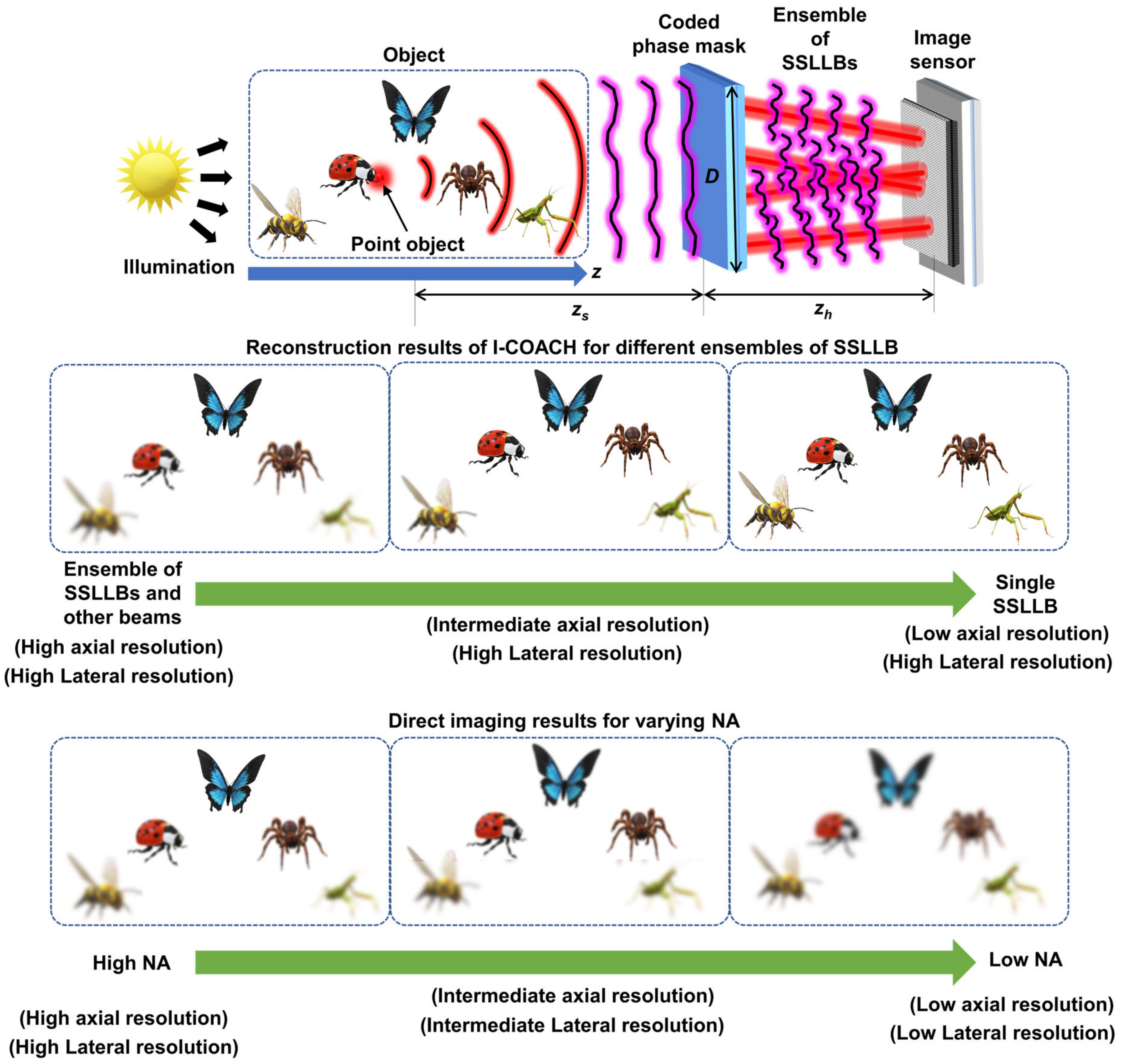
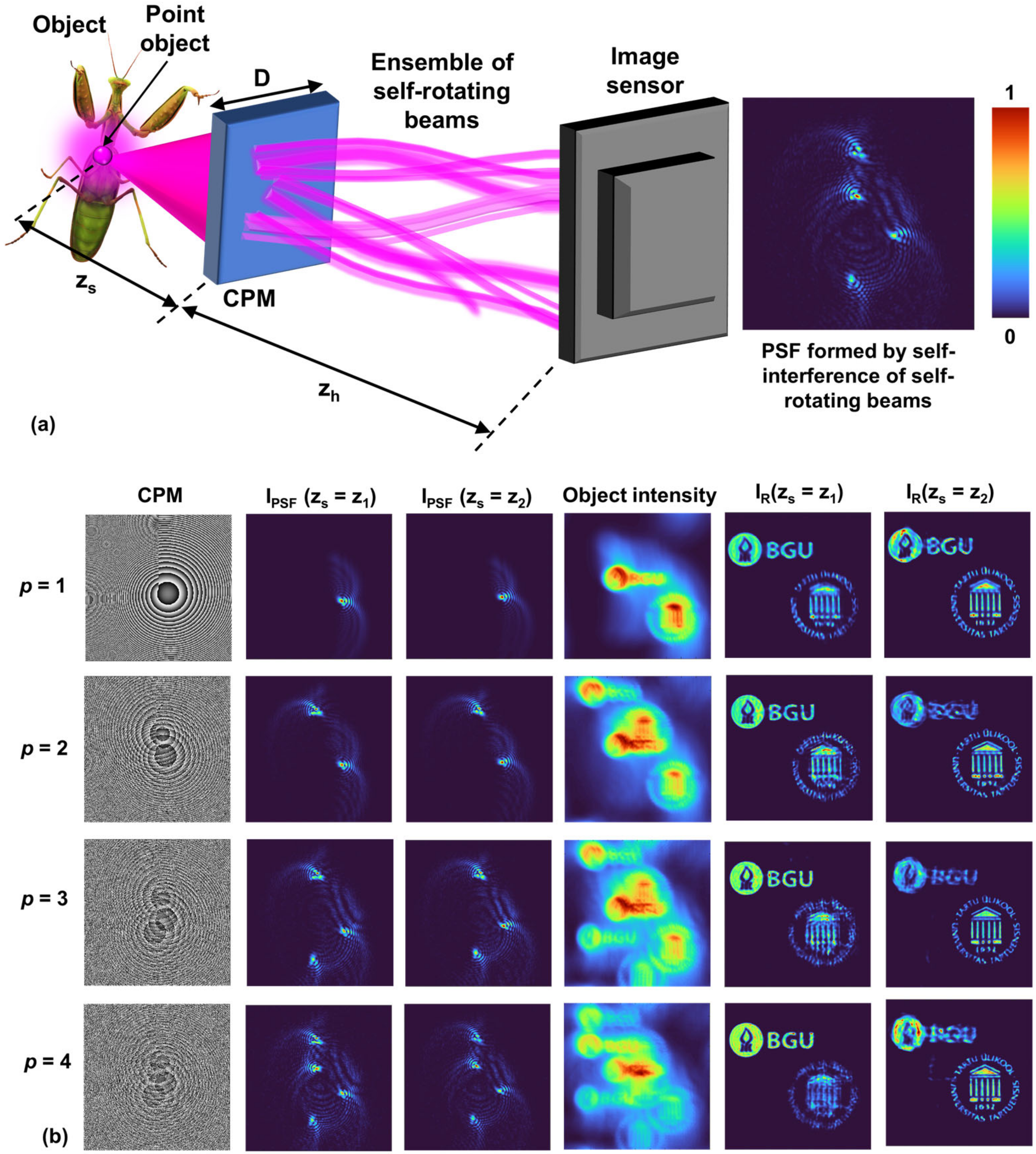
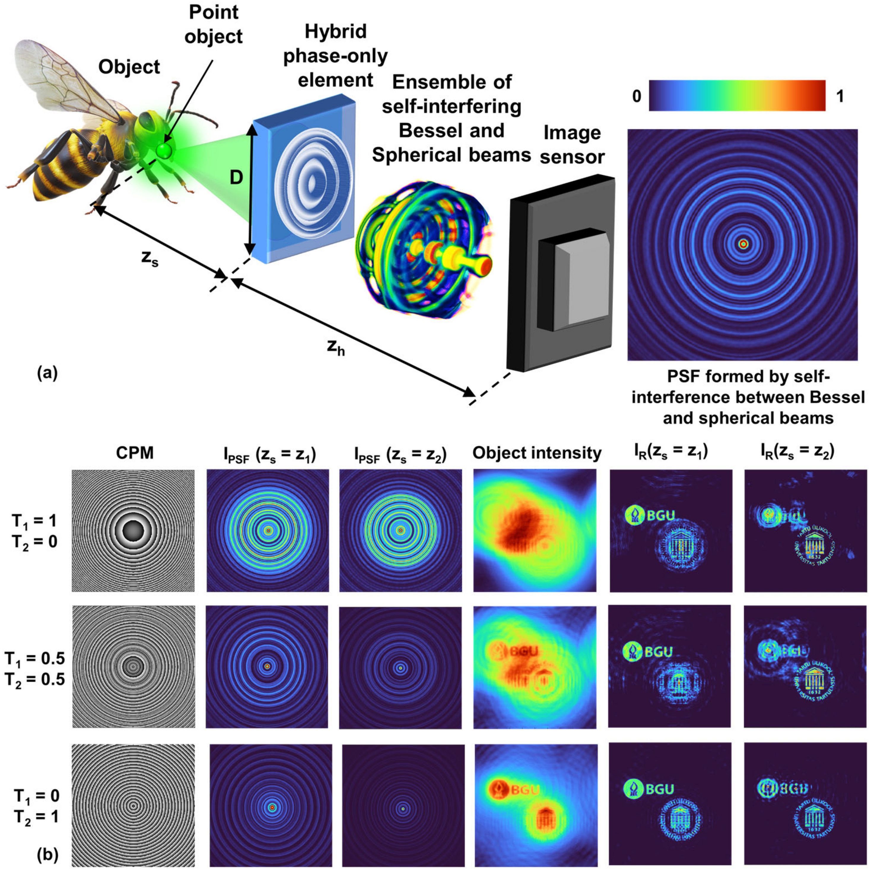
The imaging concept of I-COACH and its integration with SSLLBs are described in this section. The optical configuration of I-COACH is shown in Figure 1. Light from a point object indicated by a red dot with a glow at the head of the beetle in the top layer in Figure 1 is incident on a coded phase mask (CPM). The CPM is engineered to generate one SSLLB [6,7,8,9], or multiple SSLLBs with random 3D propagation characteristics [74,77,78,79,80], according to the system’s application, as described in the following sections. The light emitted from a point object is modulated by the CPM and recorded as the point spread function (I_PSF). The point object is then shifted to multiple axial locations, and the PSF library is recorded. After this calibration procedure, an object O is placed within the axial limits of the PSF library, and the object intensity pattern I_O is recorded. The object intensity pattern is processed with the PSF library to reconstruct 3D information about the object; 3D imaging with I-COACH is possible with a scattering mask, as demonstrated during its development in 2017 [15]. However, the depth of focus when reconstructing an I_O using a PSF recorded at a particular z is governed by the axial resolution of the system defined by its numerical aperture (NA). With an ensemble of SSLLBs, it is possible to control the depth of focus by controlling the ensemble. Tuning the depth of focus is possible even in direct imaging mode by controlling the NA, but when the axial resolution given by ~λ/NA² is changed, the lateral resolution dependent on λ/NA is also changed. The bottom two rows of Figure 1 show the depth of focus tunability in I-COACH and direct imaging. In I-COACH, when the depth of focus is changed, the lateral resolution remains unaffected, while in direct imaging, when the depth of focus is changed, the lateral resolution is affected. The mathematical formulation is presented next, which is universal to any I-COACH technique with CPM, although the recording and reconstruction methods can be different between the various I-COACH systems.

The point object located at $\overline{r_s}=(x_s,y_s)$ at a distance of z_s from the CPM emits light with an amplitude of $\sqrt{I_s}$. The complex amplitude at the CPM is given as $C_1\sqrt{I_s}L\left(\overline{r_s}/z_s\right)Q\left(1/z_s\right)$, where $Q\left(a\right)=\exp \left[i\frac{\pi a}{\lambda }\left(x^2+y^2\right)\right]$ and $L\left(\overline{s}/u\right)=\exp \left[i2\pi \left(s_{x}x+s_{y}y\right)/\left(\lambda z_s\right)\right]$ are the quadratic and linear phase functions and $C_1$ is a complex constant. The CPM transparency function is given as $\mathsf{\Psi }=\exp \left(i{\mathsf{\Phi }}_{CPM}\right)$. The complex amplitude after the CPM is given as $C_2\sqrt{I_s}Q\left(1/z_s\right)L\left(\overline{r_s}/z_s\right)\mathsf{\Psi }$, where $C_2$ is a complex constant. The $I_{PSF}$ recorded at a distance of $z_h$ from the CPM is given as

$$I_{PSF}\left({\overline{r}}_O; {\overline{r}}_s,z_s\right)=|C_2\sqrt{I_s}Q\left(\frac{1}{z_s}\right)L\left(\frac{{\overline{r}}_s}{z_s}\right)\mathsf{\Psi }\mathrm{\otimes }Q\left(\frac{1}{z_h}\right){|}^2$$

(1)

where ${\overline{r}}_O$ is the location vector in the sensor plane and ‘⊗’ is a 2D convolution operator. Equation (1) can be expressed as

$$I_{PSF}\left({\overline{r}}_O; {\overline{r}}_s,z_s\right)=I_{PSF}\left({\overline{r}}_O-\frac{z_h}{z_s}{\overline{r}}_s;0,z_s\right)$$

(2)

The object distribution at some plane can be considered a collection of points given as

$$o\left({\overline{r}}_s\right)={{\displaystyle \sum }}_{p=1}^S{a}_p\delta \left(\overline{r}-{\overline{r}}_{s,p}\right)$$

(3)

where $a_p$ is a constant of p-th point and S is the number of object points. In this study, only spatially incoherent illumination is considered; thus, the light from every point does not interfere with another; rather, the light intensities increase. Therefore, the object intensity is given as

$$I_O\left({\overline{r}}_O;z_s\right)={{\displaystyle \sum }}_{p=1}^S{a}_p{I}_{PSF}\left({\overline{r}}_O-\frac{z_h}{z_s}{\overline{r}}_{s,p};0,z_s\right)$$

(4)

The image of the object is reconstructed by a cross-correlation between the $I_O$ and $I_{PSF}$_, given as

$$\begin{array}{ll}{I}_R\left(\overline{r_R}\right)& =\iint I_O\left({\overline{r}}_O; z_s\right)I_{PSF}*\left({\overline{r}}_O-{\overline{r}}_R; z_s\right)d{\overline{r}}_0\\ & =\iint {\displaystyle \sum }_{p=1}^M{a}_p{I}_{PSF}\left({\overline{r}}_O-\frac{z_h}{z_s}{\overline{r}}_{s,p};0,z_s\right)I_{PSF}*\left({\overline{r}}_O-{\overline{r}}_R; z_s\right)d{\overline{r}}_O\\ & ={\displaystyle \sum }_{p=1}^M{a}_p\mathsf{\Lambda }\left({\overline{r}}_R-\frac{z_h}{z_s}{\overline{r}}_{s,p}\right)\end{array},$$

(5)

where Λ is a delta-like function that composes the object. The Λ size represents the lateral resolution of the system and is related to λz_h/(z_sNA) governed by the NA. The minimum limit of the axial resolution is approximately λ/NA² and the maximum limit is the focal depth of the SSLLB.

The reconstruction of an object image using regular cross-correlation between the I_O and $I_{PSF}$, according to Equation (5), is not always the optimal reconstruction method. There are numerous methods available that can be used to reconstruct object information from $I_O$ and $I_{PSF}$, such as phase-only filtering [81], Wiener deconvolution (WD) [82], nonlinear reconstruction (NLR) [18], the Lucy–Richardson algorithm (LRA) [83,84], the Lucy–Richardson–Rosen algorithm (LRRA) [68], and the recently developed incoherent nonlinear deconvolution using an iterative algorithm (INDIA) [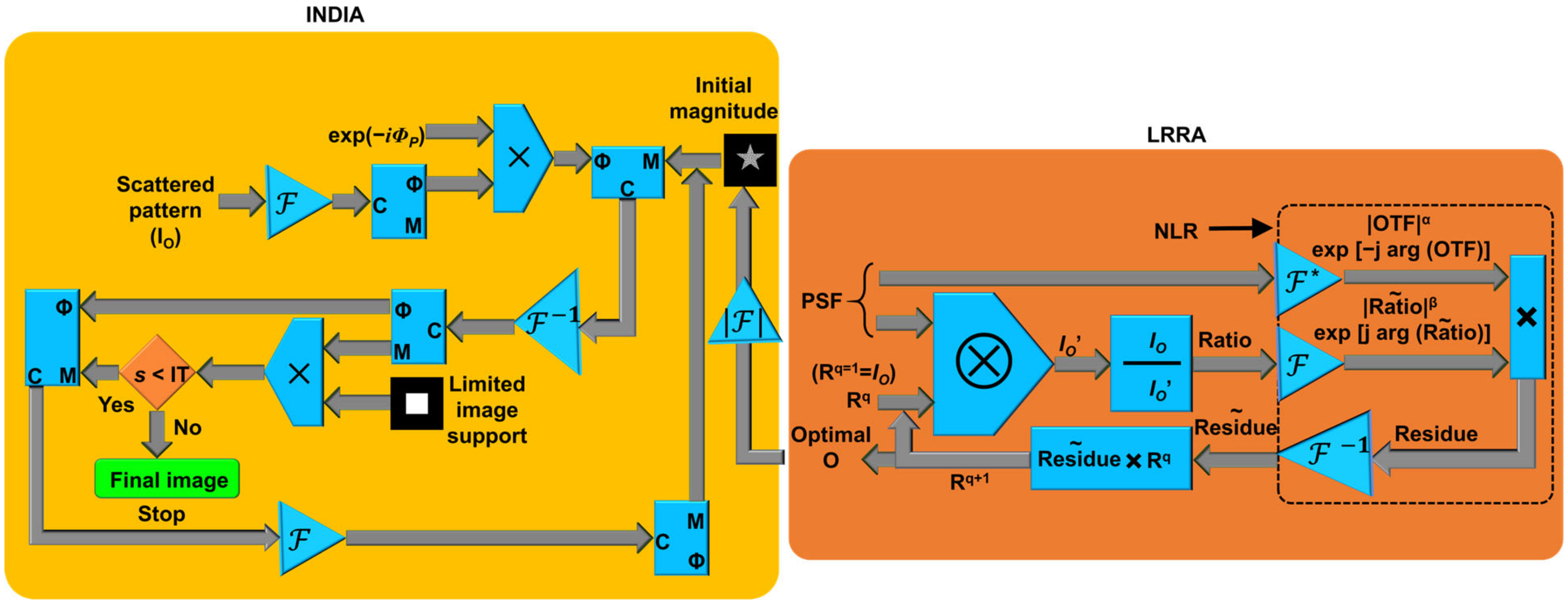85]. A comparison study was carried out between the above reconstruction methods for different types of PSFs, and both the LRRA and WD methods were found to perform better than the LRA and NLR methods. Hence, LRRA and WD are suitable for providing initial guess solutions for INDIA. Overall, INDIA is better than the other four methods.

The reconstruction approach of the INDIA is briefly discussed next. INDIA is considered the next generation of nonlinear deconvolution methods. Both the NLR and INDIA are based on the fundamental fact that most of the information about an object is in the phase of its spectrum. A nonlinear correlation between the $I_O$ and $I_{PSF}$ can be expressed with Fourier transforms as $I_R=\left|{\mathcal{F}}^{-1}\left\{{\left|{\tilde{I}}_{PSF}\right|}^{\alpha }\exp \left[i·\arg \left({\tilde{I}}_{PSF}\right)\right]{\left|{\tilde{I}}_O\right|}^{\beta }\exp \left[-i·\arg \left({\tilde{I}}_O\right)\right]\right\}\right|$, where α and β are constants whose values are searched until a certain cost function is minimized; arg(∙) refers to the phase, and $\tilde{A}$ is the Fourier transform of A. As described above, the phase information is retained, but the magnitude is tuned to achieve the minimum cost function. However, in the NLR, tuning the magnitude does not necessarily yield the optimal solution because the magnitude is not tuned pixel-wise but rather on the matrix as a whole. The parameters α and β change the entire matrix, i.e., all the pixel values by the same power. In INDIA, the magnitude is tuned pixel-wise using an iterative approach, which allows us to estimate a better solution than can be obtained from the NLR. Since it has been recently established that LRRA usually has better performance than NLR, the output of LRRA is given as the initial guess for INDIA. The LRRA was developed from the LRA by replacing the regular correlation with the NLR. A schematic of the LRRA is shown on the right side of Figure 2. LRRA begins with an initial guess of the object information, which is usually I_O (R^{q = 1}) in the first iteration (q = 1) but can be any matrix, where R^q is the solution of the qth iteration. The algorithm starts by convolving the initial guess solution $I_O$ with the recorded $I_{PSF}$, and the resulting $I_O$ is used to divide the $I_O$ to obtain the ratio. This ratio is the discrepancy between the recorded $I_O$ and the estimated $I_O$’ from the initial guess solution. This ratio is correlated with $I_{PSF}$ by the NLR to obtain the residual weight, which is multiplied by the previous solution R^{q = 1}. With every iteration, the solution approaches the ideal solution.

A schematic of the INDIA is shown on the left side of Figure 2. In the first step, the phase matrices of the spectra of $I_O$ and $I_{PSF}$ are calculated and multiplied to generate the phase information. The magnitude of the spectrum obtained by LRRA was used as the initial guess of spectral magnitude and was multiplied by the phase information, after which the inverse Fourier transform was computed. The resulting complex amplitude’s phase information is retained while a limiting window constraint is applied to the magnitude. This limiting window is the size of the object, which can be estimated either by an autocorrelation or from the result of the NLR or LRRA. The results are compared with those of direct imaging, and the above process is iterated to obtain the optimal solution. INDIA is applied to I-COACH with different types of SSLLBs.

Before the development of I-COACH, tuning axial resolution was demonstrated in COACH by hybridization methods, where a hybrid CPM is formed by combining the CPMs of COACH and Fresnel incoherent correlation holography (FINCH) [86,87,88,89] and tuning their contributions [14,29]. FINCH has a low axial resolution but a higher lateral resolution, whereas COACH has axial and lateral resolutions comparable to those of direct imaging systems with the same NA. In [14], by tuning the contributions of FINCH and COACH in the CPM, the axial and lateral resolutions were tuned between the limits of FINCH and COACH. In [29], a unique hybridization was used to achieve the high axial resolution of COACH and high lateral resolution of FINCH.

3. I-COACH with Bessel Beams

I-COACH with a CPM that can generate a random array of sparse Bessel beams was used to tune the axial resolution, independent of lateral resolution, by controlling chaos in the form of the number of Bessel beams [77]. The greater the number of Bessel beams, the greater is the axial resolution. A Bessel beam, when used as a PSF, exhibits lower axial and lateral resolutions than does the PSF of a Gaussian beam [6]. A lower axial resolution (i.e., longer DOF) arises due to the constant intensity of the Bessel beam distribution at different depths. The lower lateral resolution results from the characteristic strong sidelobes of the transverse Bessel beam distribution. In I-COACH, the reconstructed response for a point is not a Bessel distribution but a Delta-like function; due to the NLR, this Delta-like function is close to the diffraction-limited spot size, which reaches the maximum limit of the lateral resolution. The DOF of the indirect imaging mode is calculated as the width of the axial curve given by the central value (x = y = 0) of $I_{PSF}\left(z_{ref}\right){\ast }_{\beta }^{\alpha }{I}_{PSF}\left(z\right)$ along z, where ‘${\ast }_{\beta }^{\alpha }$’ indicates the NLR operation. The obtained DOF is the same as the axial length of the Bessel beam. This is because the 2D cross-correlation between mutually axially shifted Bessel beams is close to the 2D autocorrelation of a Bessel beam.

However, if there are two Bessel beams that are not collinear, then with a change in z, even though the two Bessel distributions do not change with respect to themselves, there is a change relative to each other. Therefore, $I_{PSF}\left(z_{ref}\right)$ and $I_{PSF}\left(z\right)$ are no longer the same but vary mainly due to the relative variation between the two Bessel distributions. 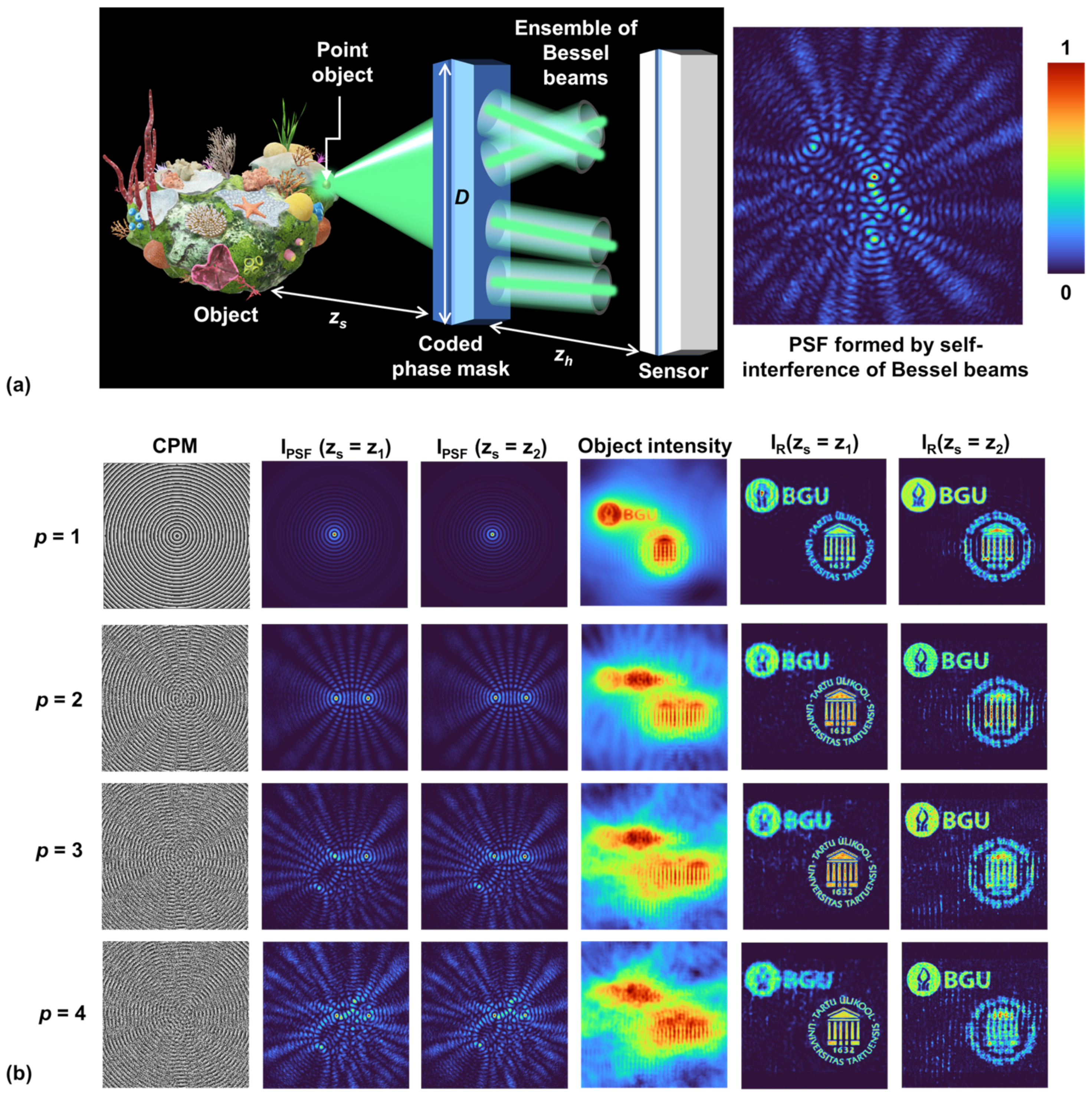When the number of Bessel distributions increases further, the difference between $I_{PSF}\left(z_{ref}\right)$ and $I_{PSF}\left(z\right)$ increases further and reaches the axial resolution limit of the direct imaging system with a Gaussian beam. However, the lateral resolutions for all the above cases remain the same. The optical configuration of I-COACH with an ensemble of Bessel beams is shown in Figure 3a.

A simulation study is shown in Figure 3b. The simulation was performed with square matrices of 250 K pixels for a wavelength of 0.65 µm, and the physical size of each pixel was set at 10 µm. The number of Bessel beams was increased in steps of 1, starting from p = 1 to 4, and the behavior was simulated for each value of p. Two test objects, namely, the logos of Ben Gurion University of the Negev and University of Tartu, were used for the simulation study. The object distances z_s for the two test objects were 37 cm and 40 cm. The recording distance z_h was 40 cm for both targets. The CPMs were designed by random multiplexing [23,26] of diffractive axicons given as $\mathsf{\Psi }={\displaystyle \sum }_{k=1}^p\exp \left[-i\left\{\frac{2\pi }{{\mathsf{\Lambda }}_{k_1}}\sqrt{{\left(x-a_{k_1}\right)}^2+{\left(y-a_{k_2}\right)}^2}\right\}\right]\exp \left(i\frac{2\pi }{{\mathsf{\Lambda }}_{k_2}}x\right)\exp \left(i\frac{2\pi }{{\mathsf{\Lambda }}_{k_3}}y\right)\mathrm{Mask}\left(k\right)$ with different locations and linear phases, where ${\mathsf{\Lambda }}_{k_1}$, ${\mathsf{\Lambda }}_{k_2}$ and ${\mathsf{\Lambda }}_{k_3}$ are the constants of the axicons in the x and y directions, respectively; $a_{k_1}$ and $a_{k_2}$ are the shifts in the x and y directions, respectively; and Mask(k) is the kth binary random mask, which is orthogonal to any other Mask(m) k ≠ m. There are different approaches for designing mutually exclusive binary random matrices. In our study, a normalized grayscale random matrix was created in the first step. Mutually exclusive binary random matrices are created by assigning the pixel locations of the grayscale random matrix with different ranges of values to one and zeros to other locations. For instance, for p = 4, four binary mutually exclusive matrices are created by selecting the pixels of the grayscale random matrix with values of 0 to 0.25, 0.25 to 0.5, 0.5 to 0.75, and 0.75 to 1 such that the sum of all the mutually exclusive random matrices yields a uniform matrix with all the pixels set to a value of 1. For p = 1, the Mask function is uniform. The images of the phase mask, I_PSFs at two distances, the object intensity pattern for the two test objects at locations z₁ and z₂, and the reconstruction results using INDIA with the output of LRRA as the initial guess and approximately ten iterations are shown in Figure 3b.

4. I-COACH with Airy Beams

The optical configuration of I-COACH with an ensemble of Airy beams is shown in Figure 4a. Airy beams have focal characteristics similar to those of Bessel beams but exhibit nonrectilinear propagation paths. While most studies with Airy beams involve a coherent light source [90,91,92], there are also few studies with incoherent sources that demonstrate that the focal characteristics are quite similar to those of a coherent source [79,93]. Like Bessel beams, Airy beams are not radially symmetric and have peculiar asymmetric distributions, which give rise to sidelobes in correlation if sufficient diversity is not introduced in the ensemble. In addition to designing cubic phase masks, additional unique shifts and coordinate rotations are introduced. The CPM for generating an ensemble of Airy beams is given as $\mathsf{\Psi }={\displaystyle \sum }_{k=1}^p\mathrm{Mask}\left(k\right)\exp \left[-i\frac{2\pi }{\lambda }\left\{{\xi }_k{\left(x_k+a_{k_1}\right)}^3+{\eta }_k{\left(y_k+a_{k_2}\right)}^3\right\}\right]$, where $x_k=x_{0}cos{\theta }_k+y_{0}sin{\theta }_k$, $y_k=y_{0}cos{\theta }_k-x_{0}sin{\theta }_k$, ${\xi }_k$, and ${\eta }_k$ are the scaling factors along the x and y directions, respectively. The simulation conditions are similar to those for Bessel beams. The images of the phase masks, I_PSFs for z₁ and z₂, and I_Os and I_Rs corresponding to z₁ and z₂ are shown in Figure 4b.

The difference between using an ensemble of Bessel beams and Airy beams is that with Airy beams, it is possible to transversely shift images of the objects differently along the z-axis. This property arises due to the nonrectilinear propagation of Airy beams. This effect is observed when a single Airy beam is used. Two cases for two CPMs to demonstrate the push and pull effects with an Airy beam are demonstrated in Figure 5. The distance between the two objects was increased to 15 cm. In row 1, the objects are pushed away from one another, while in row 2, the objects are pulled toward one another in the transverse direction. This property allows us to separate the transversely overlapped object information corresponding to two axial planes.

5. I-COACH with Self-Rotating Beams

A self-rotating beam is a recently discovered optical beam that has a long focal depth where the intensity distribution rotates around an axis [8]. While the self-rotating beam proposed in [8] involves a complicated design with topological charges, such self-rotation beams can also be generated following the conventional methods of designing lenses with a long focal depth, such as axilens [94]. In the axilens, there is a radial dependent focal length, i.e., the Fresnel lens is divided into circular zones, and each zone has a different focal length. Consequently, the resulting intensity distribution is similar to that of a Bessel distribution. To design a diffractive element for the generation of a self-rotating beam, the focal length is changed with respect to the angle. For an optical configuration, as shown in Figure 6a, the focal length is given as $f\left(\theta \right)=f_0+\frac{\Delta f}{2\mathsf{\pi }}\theta$, where Δf is the depth of focus and f₀ is the focal length of the sector with θ = 0. The diffractive element is partitioned azimuthally with every infinitesimal sector designed for a focal length between f₀ and f₀ + Δf. For the optical configuration shown in Figure 6a, $\frac{1}{f\left(\theta \right)}=\frac{1}{z_s}+\frac{1}{z_i} ,$ and the image distance is $z_i\left(\theta \right)={\left(\frac{1}{f\left(\theta \right)}-\frac{1}{z_s}\right)}^{-1}$. The phase of the diffractive element is given as ${\mathsf{\Phi }}_{FZL-AVF}\left(R,\theta \right)\approx \frac{-2{\pi }^2{R}^2}{\lambda \left(2\pi f_0+\Delta f\theta \right)}$. The CPM is designed to create an ensemble of self-rotating beams with different values of Δf and f₀. The transparency function of the CPM is given as $\mathsf{\Psi }={\displaystyle \sum }_{k=1}^p\mathrm{Mask}\left(k\right)\exp \left[-i\left(\frac{-2{\pi }^2{R}^2}{\lambda \left(2\pi f_0\left(k\right)+\Delta f\left(k\right)\theta \right)}\right)\right].$ The simulation study was carried out under the same conditions as those used for the Bessel and Airy beams, and the results are shown in Figure 6b. Images of the CPMs, I_PSFs at the two axial locations, and I_O and I_Rs at the two axial locations are shown in columns 1 to 6, respectively. Once again, the change in axial resolution is independent of lateral resolution for different numbers of self-rotating beams. The performance of an ensemble of self-rotating beams is similar to that of an ensemble of Bessel beams because the paths of the beams are rectilinear and because of the asymmetry in the intensity distributions. In [79], a higher SNR was reported for self-rotating beams than for Airy beams when the NLR was used for reconstruction. However, with LRRA and INDIA, the SNRs obtained for the Airy beams and self-rotating beams are similar, as shown in Figure 5 and Figure 6.

6. Depth-of-Field Engineering

DOF engineering means that the imaging system is designed to image objects located at different depths from the system in different ways such that their images appear in the output or disappear according to their axial location. In the DOF engineering scheme, the object space is divided into several isolated volumes along the longitudinal axis with different lengths. Objects located at a certain volume are selectively imaged with the same sharpness regardless of where the object is located inside the volume, where the length of the volume determines the DOF of the system for all objects inside this volume. Objects positioned outside any volume are not imaged at all, meaning that their image does not appear in the system’s output. By using DOF engineering, one can selectively image objects from any chosen volume separately or simultaneously with other volumes. These choices can be performed in the digital reconstruction stage after recording the object hologram, and images from different volumes can be transversely shifted to avoid overlap of images from various volumes. In this section, we briefly summarize the work of DOF engineering in I-COACH imaging systems based on the PSF of SSLLB of limited nondiffracting beams [74].

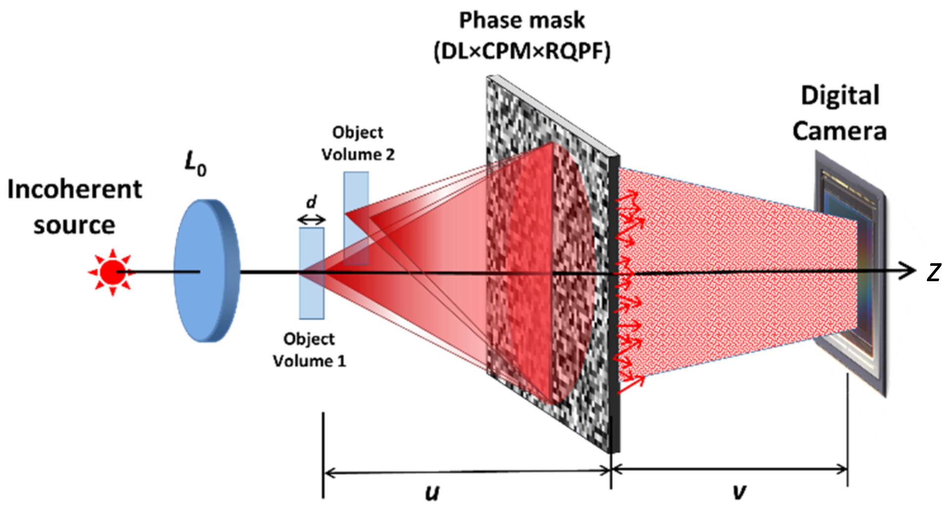
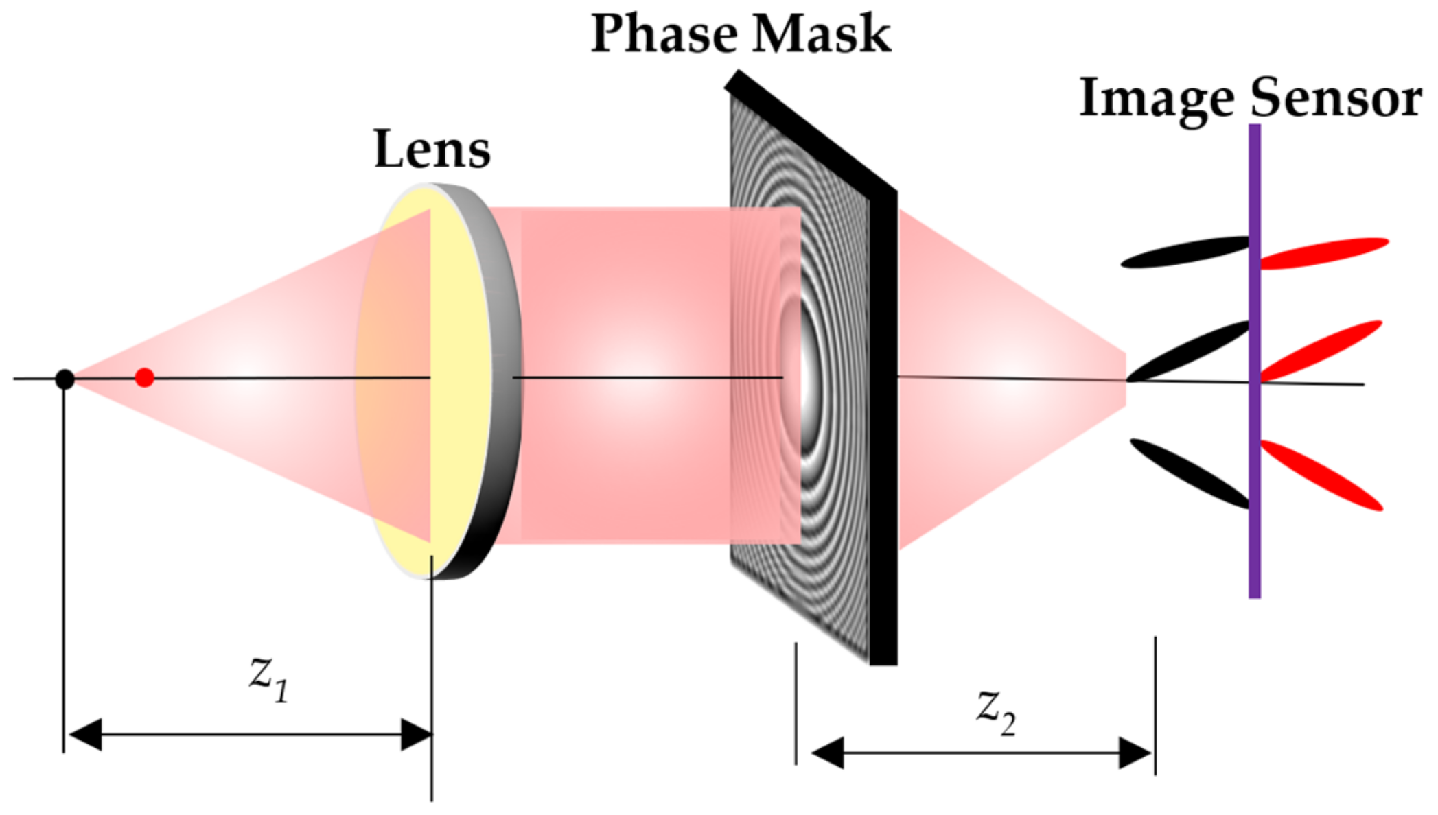
The DOF engineering proposed in [74] is performed by introducing radial quartic phase functions (RQPFs) into the aperture of the I-COACH system, as schematically shown in Figure 7. The use of RQPFs for creating limited nondiffracting beams was proposed in [9] (with a different term than RQPF). The mathematical justification of using RQPF is based on the McCutchen theorem [75]. According to the McCutchen theorem, there is a Fourier relation between the radial distribution of a transverse aperture of a focusing light field and the longitudinal field distribution around the focal point, where the focal point is the axis origin of this longitudinal field distribution. In formal notation, the 2D focusing aperture is $g\left(r,\theta \right)$, where $\left(r,\theta \right)$ are the polar coordinates of the aperture and a focusing aperture means that $g\left(r,\theta \right)$ is illuminated by a converging spherical wave. The aperture radial distribution is $t\left(r\right)={{\displaystyle \int }}_0^{2\pi } g\left(r,\theta \right)d\theta .$ According to the McCutchen theorem, the intensity along the z-axis satisfies the relation $I\left(z\right)\propto {\left|\mathcal{F}\left\{t\left(\rho \right)\right\}\right|}^2$, where $\mathcal{F}$ indicates a one-dimensional Fourier transform, the focal point is the origin of the longitudinal axis z, and $\rho =r^2$. Recalling that the goal is to create a limited nondiffracting beam, $I\left(z\right)$ should be a constant along a limited range. In a table of Fourier transforms, there are two well-known functions for creating a constant intensity $I\left(z\right)$. One is the Dirac delta function $t\left(\rho \right)=\delta \left(\rho -{\rho }_o\right)$, where ${\rho }_o$ can be any constant between zero and the squared radius of the aperture. This delta function dictates an annular aperture for $g\left(r,\theta \right)$, and when $g\left(r,\theta \right)$ is illuminated by a focusing beam, the resulting beam near the focus is the well-known Bessel beam [76], which is indeed a limited nondiffracting beam. The other optional function to have a constant $I\left(z\right)$ is the quadratic phase function in $\rho$, which is a quartic phase function in $r$, i.e., $t\left(\rho \right)=\exp \left(i2\pi {\rho }^2/q^4\right)=\exp \left(i2\pi r^4/q^4\right)$, where $q$ is a real constant. This function of $t\left(\rho \right)$ is a pure phase function, and if $g\left(r,\theta \right)=\exp \left(i2\pi r^4/q^4\right),$ this aperture, unlike the annular aperture, does not absorb light when it is introduced as a mask in the optical system. Therefore, RQPF has become an attractive alternative to narrow annular apertures or any other light-absorbing apertures. Note that because the McCutchen theorem is valid only for focusing beams, to create a limited nondiffracting beam with RQPF, one needs to illuminate the RQPF with a focusing beam. Alternatively, two attached components, an RQPF and a thin spherical lens, can be illuminated by a spherical wave such that a converging spherical wave is emitted from the attached components, and according to the McCutchen theorem, the limited nondiffracting beam starts from the focal point of the converging wave.

The simplest case of DOF engineering is the extension of the imaging system’s DOF, which means that there is only a single volume instead of the multivolume scheme mentioned above, as shown in Figure 7. The way to extend the DOF proposed in [74] is to integrate a single RQPF into the I-COACH system with a PSF of sparse dots [22]. Without the RQPF, the I-COACH system with a PSF of sparse dots has an aperture of two optical elements. The first element is the CPM, which creates a randomly distributed pattern of several dots. The other element is a converging lens that guarantees that the dots are obtained on the camera plane. The RQPF, which is now the third mask in the combined coded aperture, extends the length of the dots and extends the DOF. In principle, various optical masks can be introduced into the system separately; however, in the present case [74], all the elements appear in a single-phase mask displayed on the SLM, where the mask has a phase distribution that is a multiplication of the three phase functions as follows $\exp \left[i\left(2\pi r^4/q^4-\pi r^2/\lambda f+\mathsf{\Phi }\left(r\right)\right)\right]$, where λ is the central wavelength and $\mathsf{\Phi }\left(r\right)$ is the chaotic function of the CPM, which creates the randomly distributed dots [22]. The focal distance f of the positive diffractive lens is set to satisfy the imaging relations between the object and camera planes. In formal notation, the focal length f and the gaps between the object and the SLM u and between the SLM and camera v fulfill the relation 1/f = (1/u) + (1/v), known as the imaging equation. When the RQPF is attached to the CPM and to the converging lens, the PSF is changed from some number of focusing dots to the same number of rods that remain in focus along a limited interval; consequently, the DOF of the dots is extended. Therefore, any object point located in the axial range of the DOF yields approximately the same dot pattern on the camera. Moreover, because of the extended DOF of the PSF, any object located in the axial range of the DOF is approximately imaged with the same sharpness. The phase function of the RQPF, $\exp \left(i2\pi r^4/q^4\right)$, extends the randomly distributed dots from a focal point to an intensity rod shape, where q is the constant dictating the extent of the rod and hence the length of the DOF. In other words, the RQPF generates limited nondiffracting beams on the camera plane with an approximately constant intensity along a limited gap and a relatively narrow beam-like profile at any lateral plane. According to [74], the DOF of the system is $\lambda u^2{W}^2/\left(q^4-\lambda u{W}^2\right)$, where W is the diameter of the aperture. The DOF initial point and the length of the rods are determined by modifying the focal length of the lens f and the constant q of the RQPF, respectively.

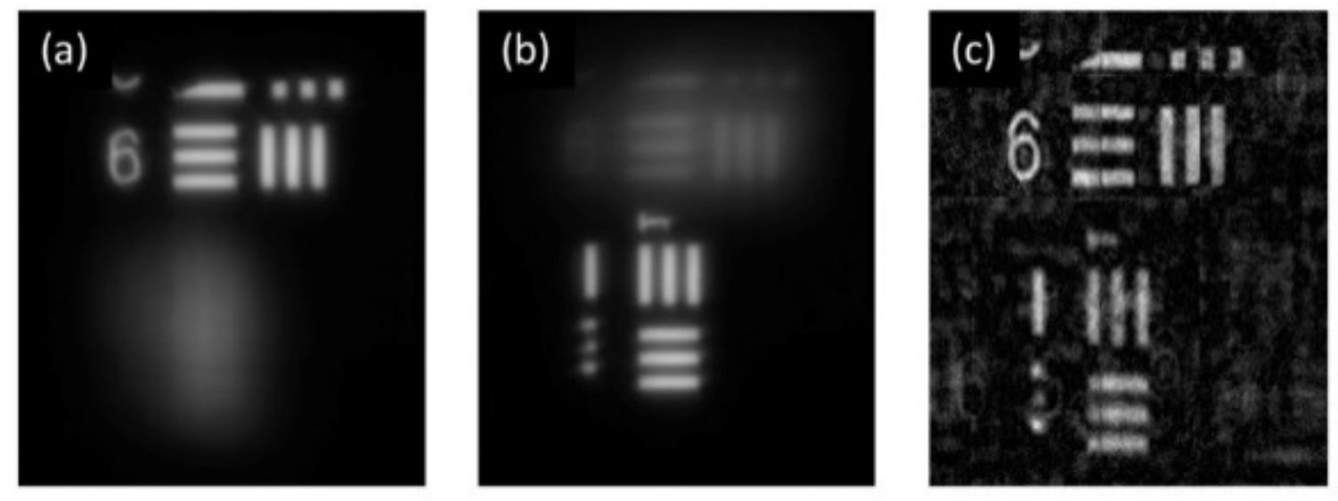
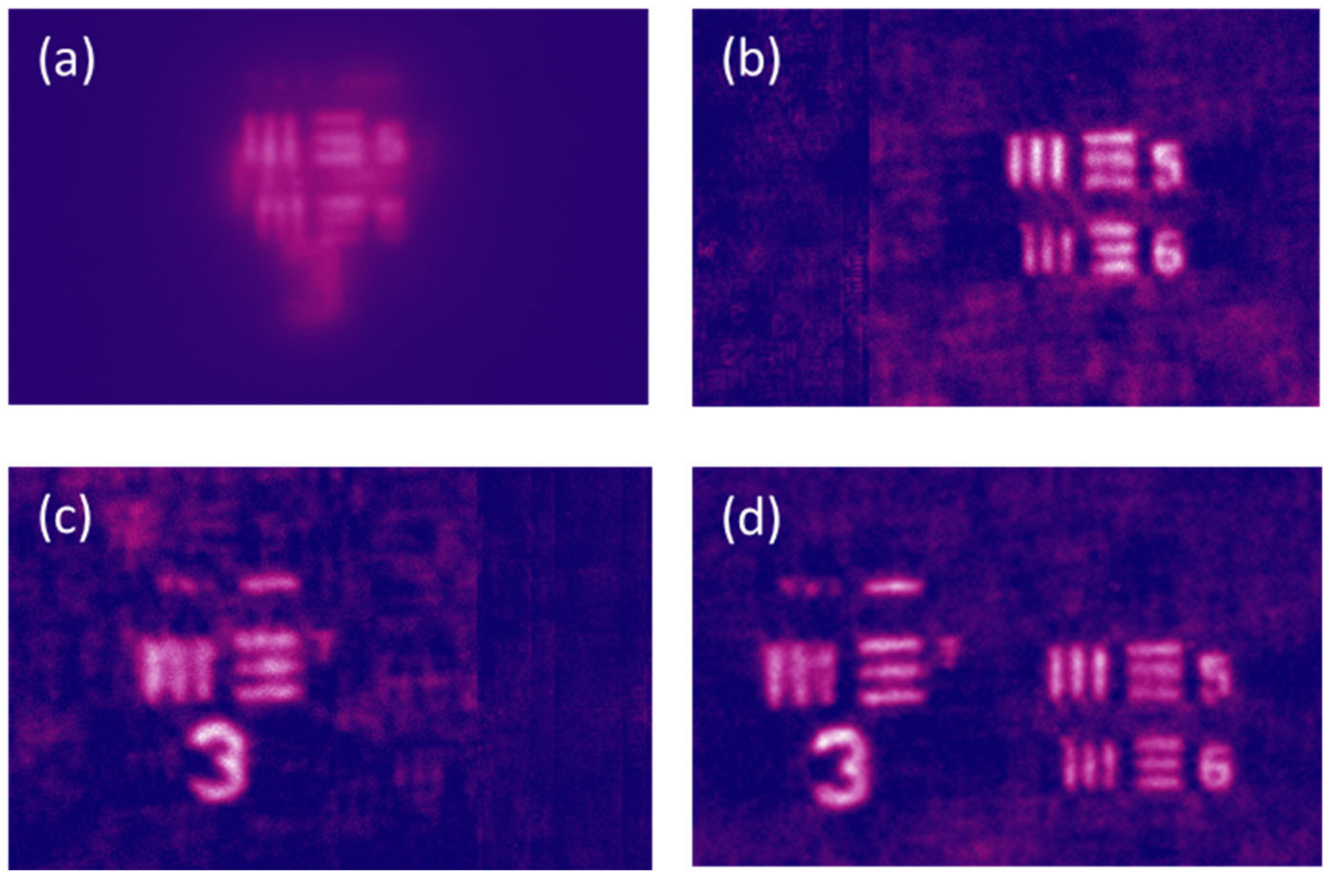
The DOF extension method is demonstrated by an optical setup, shown in Figure 7. Two objects located at different distances from the coded aperture are considered positioned at each edge of the observed volume. The objects are positioned at distances of 24 and 26 cm from the coded aperture displayed on the SLM. Both targets are different parts of the USAF transmission resolution chart; one is element 6 of Group 2, and the other is element 1 of Group 3. A distance of 22 cm was set between the camera and the SLM. Displaying on the SLM, only a single diffractive positive lens creates a direct image of the targets on the camera plane (shown in Figure 8a,b), where each time, a different value of the focal length satisfies the imaging equation for each object located at a different depth. For direct imaging, Figure 8a,b clearly show that the longitudinal distance between these objects was too long to be the focus of both objects during the same camera shot. The I-COACH PSF contained a CPM that produces 10 randomly distributed dots on the detection plane. The I-COACH-recovered image is shown in Figure 8c, which reveals that both objects are in focus without a resolution reduction. According to these results, the system is engineered to have a DOF of 3 cm.

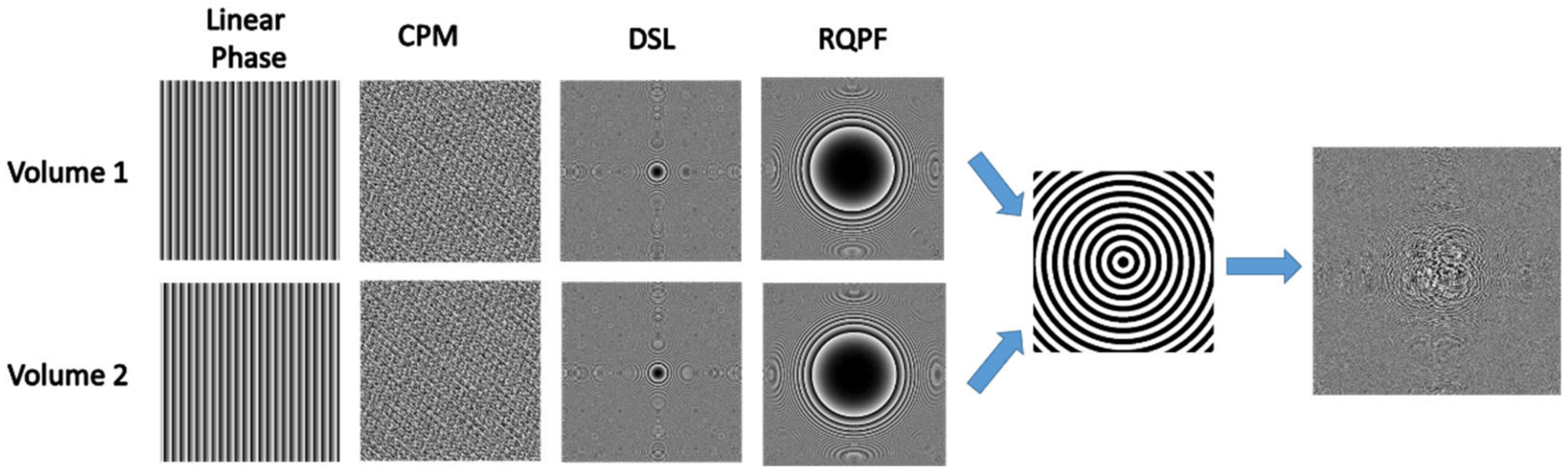
Next, we describe a more advanced technique of DOF engineering in which objects from more than a single volume are imaged. Objects from the two volumes shown in Figure 7 are processed such that two situations are considered. In the first situation, in-focus imaging is shown first for objects within volume No. 1 and then for those within volume No. 2, where other objects located outside these volumes are always out-of-focus. In the second situation, two images belonging to two different volumes are reconstructed simultaneously with a lateral shift between them. Moreover, they are reconstructed from the same object hologram used in the first situation. In other words, different reconstruction operations performed on the same hologram yield different images, and there is no need to record a different hologram for every image. The image lateral shift is meaningful for targets positioned on the same line of sight and consequently overlapping each other. From the SLM, Volume 1 was positioned at an interval of 16.9–18.5 cm, and Volume 2 was positioned at 22.2–24.7 cm. The goal of the first situation is to recover an image from a single recorded hologram, an image belonging only to either volume 1 or 2. Because volumes 1 and 2 are located at different depths, different sets of parameters are needed for the three-phase components of the RQPF, lens, and CPM. The two sets of phase elements can be multiplexed either in time or in space, where time multiplexing means recording more than a single hologram, and space multiplexing means a reduced SNR in comparison to time multiplexing. To have one phase aperture on the SLM and to record a single hologram, for objects from both volumes, two different sets of three phase masks were spatially multiplexed, as shown in Figure 9. Binary circular gratings with a ring width of 30 pixels, as shown in the fifth column of Figure 9, were used to divide the SLM area between the two sets of phase components, each for every volume. Specifically, the phase masks corresponding to volume 1 were displayed on white rings, and those corresponding to volume 2 were displayed on black rings. Therefore, the final coded aperture has the capability to image targets from both volumes. Further linear phase masks, shown in the first column of Figure 9, were added to the two sets to transversely separate the images of the targets from the two volumes. For the image lateral shift, horizontal linear phase shifts of +0.9° and −0.9° were introduced to the phase masks of volumes 1 and 2, respectively. These linear phases deflect the light beyond the SLM in two opposite directions; hence, images of objects from the two volumes are shifted in opposite directions.

The imaging results for the two volumes in the abovementioned two situations are described in the following. Elements 5–6 of group 3 (12.7–14.25 lp/mm) and element 1 of group 3 (8 lp/mm) of the USAF resolution chart were positioned in volumes 1 and 2, respectively. Figure 10a shows direct images of the objects where the image from volume 2 is in-focus and the image from volume 1 is out-of-focus. The images of the two different volumes overlap each other since they are located on the same sightline. This disturbing overlap can be avoided using DOF engineering, as demonstrated in Figure 10b–d. Two different PSFs corresponding to volumes 1 and 2 were formed digitally with the same values of scattering and number of dots. Separate reconstructed images of the targets from the two volumes are shown in Figure 10b,c. Cross-correlation with the corresponding PSF of each volume yields these two different images. The results shown in Figure 10b,c illustrate the abovementioned first situation, where the image in Figure 10d describes the second situation. The goal of the experiment shown in Figure 10d was to reconstruct images of the targets from both volumes via a single digital reconstruction from the same hologram used for the first situation. Figure 10d simultaneously shows in-focus images from the two different volumes with transverse separation of the images. The ability of DOF engineering to reconstruct images in different volumes from a single hologram, as well as to achieve lateral separation between the images from the different volumes, has been successfully demonstrated.

7. Image Sectioning from a Single Viewpoint

In this section, we describe a different application for limited nondiffracting beams based on the work published in [41]. The application of this section is image sectioning in a 3D scene from a single viewpoint. Image sectioning means that an image of a single lateral slice of the whole 3D object scene appears in the output, and the out-of-focus distribution from the object outside the considered slice is suppressed as much as possible. Image sectioning is considered a special case of DOF engineering in which the entire 3D scene is considered as the only processed volume, while the system aims to minimize the DOF for each lateral slice. The sectioning tools proposed in [41] are similar, but not identical, to those used in the DOF engineering [74] discussed in the previous section. Here, we consider three types of phase elements, RQPF, linear phase, and diffractive lens, used to satisfy the Fourier relation between the coded aperture plane and the detection plane. The lens appears in combination only once, where several pairs of RQPFs and a linear phase are multiplexed on a single-phase mask together with the lens. Each linear phase has a random vector $\overline{a}$ = (a_x,a_y) that multiplies the spatial variables (x,y). By combining a diffractive lens with several pairs of RQPFs and linear phases, a set of parallel rods is generated on the camera plane in random order. The transverse location of each rod is determined by the corresponding linear phase. To make this PSF capable of performing image sectioning, one needs to tilt each rod at a different angle relative to the z-axis. Therefore, the proposed method is called sectioning by tilted intensity rods (STIR). As described and demonstrated in [41], a shift between the centers of each RQPF and the center of the lens causes a tilt of the rod by an angle relative to the z-axis. In formal notation, the aperture of the I-COACH system is a multiplication of the positive lens with several shifted RQPFs, each of which is multiplied by a different linear phase as follows:

$$T\left(\overline{r}\right)=\exp \left(-\frac{i\pi {\left|\overline{r}\right|}^2}{\lambda f_2}\right){{\displaystyle \sum }}_{k=1}^K{\Theta }_k\left(\overline{r}\right)\exp \left[\frac{i\pi }{b}{\left|\overline{r}-{\overline{d}}_k\right|}^4\right]\exp \left(i2\pi {\overline{a}}_k·\overline{r}\right),$$

(6)

where $\overline{r}=\left(x,y\right),$ f₂ is the focal length of the diffractive lens, K is the number of tilted beams in the PSF, b is the parameter of the RQPFs, which dictates the length of the rods, and ${\overline{a}}_k=\left(\sin {\alpha }_{x,k},\sin {\alpha }_{y,k}\right)/\lambda$ is the vector of the linear phase parameters of the kth beam, generating K different shifts from the origin of the detection plane of $f_2\sin {\alpha }_{x,k}$ horizontally with a vertical shift of $f_2\sin {\alpha }_{y,k}$ to each kth rod. ${\Theta }_k\left(\overline{r}\right)$ are the orthogonal binary functions that randomly jump between the values 1 and 0 and satisfy ${{\displaystyle \sum }}_{k=1}^K{\Theta }_k\left(\overline{r}\right)=N\cdot M,$ assuming that the I-COACH aperture is displayed on a matrix of N × M pixels. When the phase-only mask of Equation (6) is illuminated with a plane wave, a set of K tilted rods is randomly distributed over the detection plane. All the rods begin from the back focal plane of the diffractive lens and extend along a finite length dependent on the constant b. Each k-th rod has its own vector shift ${\overline{d}}_k$; hence, each rod is tilted at a different angle and orientation. Therefore, when the point object moves back and forth inside the object volume, in every axial location, the camera records a different PSF of dots, as shown in Figure 11. Every PSF has the same number of dots, but their arrangement on the detection plane is different because of the different tilts of each rod. The system stores these entire PSFs in the PSF library. In the reconstruction stage, when one PSF from the library is cross-correlated with the object hologram, only one slice of the 3D object is imaged on the output plane, the slice that corresponds to the chosen PSF.

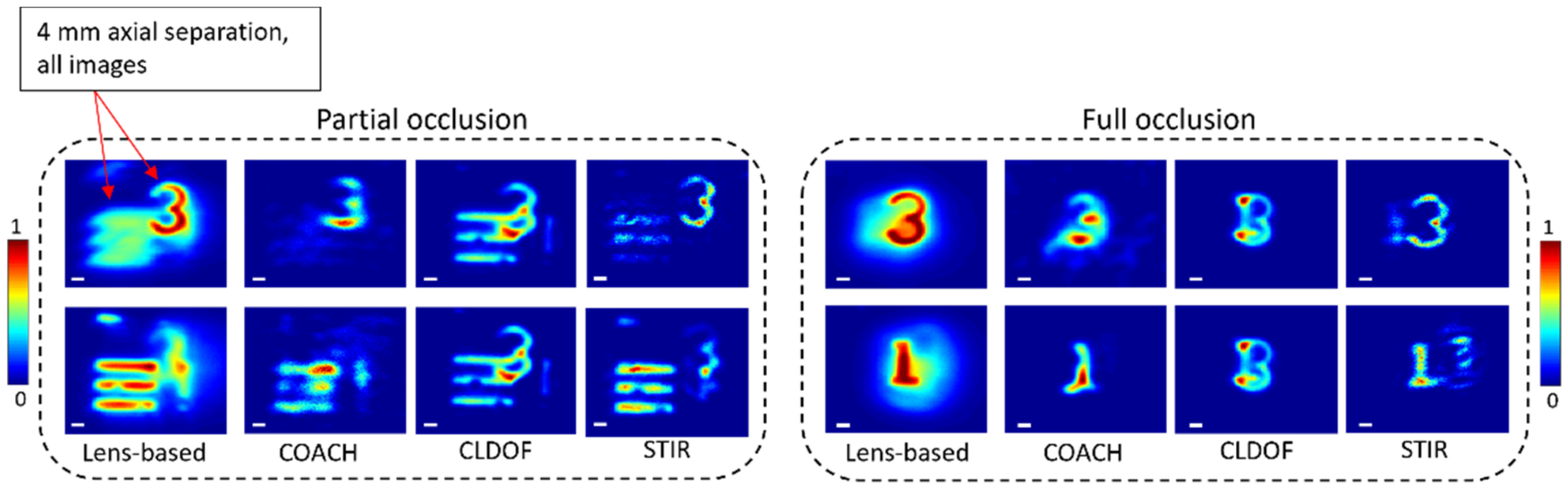
In the following experiment, the imaged scene was designed so that an image from one plane obscures that from another plane by changing the lateral locations of the objects. In such a scenario, successful reconstruction of all objects located at different planes is considered image sectioning, a challenging task with data captured from only a single viewpoint without scanning along the z-axis. Figure 12 on the left shows the image reconstruction of each plane of interest based on a single hologram, along with lens-based imaging. Here, the compared holographic methods are I-COACH, STIR, and I-COACH with long DOF (CLDOF), which are accomplished by the PSF of straight (untitled) light rods, as discussed in Section 6 and in [74]. The CLDOF was incorporated into the experiment to emphasize the significance of the inclination of light beams for sectioning. Obviously, STIR accomplishes sectioning of the 3D scene, whereas all the other methods do not. Apparently, the occluded signal cannot be recovered from an I-COACH hologram without considerable noise, and the recovered distorted signals contain undesired traces of the object that resides in the adjacent plane. On the other hand, in STIR, the multiple and pseudorandom transverse dislocations between adjacent planes enable us to fully recover the occluded image, leading to a complete and accurate reconstruction of objects from each plane of interest. Like in STIR, CLDOF also extends the in-focus range and captures a hologram that contains multiple planes of interest, in focus simultaneously. However, in CLDOF, all the image replicas have the same spatial distribution as that of the 3D scene. Hence, the CLDOF cannot distinguish the different planes within the volume, and it recovers all the structures with the same quality. As an additional trait, we inspected how each method would perform under full overlap between the objects from each plane. In this demonstration, the vertical grating was replaced by the digit ‘1’, and the transverse location was set accordingly. Figure 12 on the right shows that the tilted beam approach of STIR can perform an optical sectioning procedure, exposing the fully obscured object with high fidelity. On the other hand, COACH and CLDOF cannot distinguish multiple planes of interest, and the reconstruction results are highly distorted.

8. Sculpting Axial Characteristics with Incoherent Imagers

Recently, a modified approach to tune the axial resolution of an incoherent imaging system without affecting the lateral resolution was proposed using an ensemble of only two beams, one with high and the other with low focal depths [80]. This method was based on the hybridization method, which was demonstrated in 2017 to combine the properties of FINCH and COACH [14]. Compared with COACH, FINCH has a higher lateral resolution and a lower axial resolution, and COACH has a lower lateral resolution and a higher axial resolution. To create an incoherent digital holography system that has the mixed characteristics of FINCH and COACH, a hybridization method was developed. In that hybridization approach, the phase masks of FINCH and COACH were combined, and the parameter α was used to tune the contributions of the two phase masks: α = 0, FINCH and α = 1, COACH; for other values of α, mixed properties of FINCH and COACH were obtained. However, in that study [14], the lateral resolution was not constant but rather varied when the axial resolution was varied. Since the hybridization method was developed in the initial stages of COACH, three camera shots were needed.

To demonstrate the tuning of axial resolution without affecting lateral resolution, two-phase masks, namely, a diffractive axicon and a diffractive lens, were combined using two parameters, namely, T₁ and T₂. The CPM function is given as $\mathsf{\Psi }\approx \exp \left[-i\pi T_1{\left(\lambda f\right)}^{-1}\left(x^2+y^2\right)\right]+\exp \left[-i2\pi T_2{\mathsf{\Lambda }}^{-1}\sqrt{x^2+y^2}\right]$, where f is the focal length of the diffractive lens, Λ is the period of the diffractive axicon, $0\le T_1\le 1$ and $0\le T_2\le 1$. When T₁ = 0 and T₂ = 1, the CPM is a diffractive lens; when T₁ = 1 and T₂ = 0, the CPM is a diffractive axicon; and for other combinations, mixed properties of the diffractive lens and axicon were obtained. In the original study [80], random multiplexing was avoided using a phase retrieval algorithm called the transport of amplitude into phase based on the Gerchberg–Saxton algorithm (TAP-GSA). This approach improved the SNR and light throughput, as described in [80,95]. Several previous studies [96] showed that it is possible to use the phase mask obtained from the phase of the complex amplitude of the sum of phases of diffractive axicon and diffractive lens instead of random, or other, multiplexing by TAP-GSA.

The simulation conditions are similar to those used for the Airy, Bessel, and self-rotating beams. Three cases were considered: (T₁,T₂) = (1,0), (T₁,T₂) = (0,1), and (T₁,T₂) = (0.5,0.5); namely, a diffractive lens, a diffractive axicon, 50% of the lens and 50% of the axicon. The images of the CPMs, the I_PSFs at the two axial locations, and the I_O and I_Rs at the two axial locations are shown in columns 1 to 6 of Figure 13, respectively. As shown in the figures, the axial resolution decreases as we move from the lens to the axicon. By choosing appropriate values of T₁ and T_2, it is possible to sculpt the axial characteristics. Compared to previous cases in which Airy, Bessel, or self-rotating beams were used, the proposed study requires only two beams, which simplifies the design. The above approach also improves the SNR compared to an ensemble of beams with a high focal depth because only one random matrix is needed instead of many, resulting in reduced scattering effects.

9. Conclusions

This review addresses the successful integration of two unrelated technologies. On the one hand, a well-known technique beginning in the 1990s, longitudinal beam shaping [97], was used mainly for directing laser beams in free space. On the other hand, beam shaping technology in general and SSLLB in particular were integrated into a recently proposed imaging technology known as I-COACH [15,16,17,18,19,20,21,22,23,24,25,26,27,28,29,30,31,32,33,34,35,36,37,38,39,40,41,42,43,44,45,46]. As described in this review, this integration has solved several different problems and has been implemented in various imaging applications. Most examples of practical applications, demonstrating the real-world utility of these techniques, exist in the microscopy field [58,88,91]. These proposed techniques provide the capabilities of 3D imaging to the new microscopes.

Once again, we see that a combination of two unrelated techniques can yield a new technology with superior capabilities that do not exist in other technologies. This new technology still has much to be improved in terms of hardware and software. In hardware, better SLMs with more and smaller pixels will undoubtedly improve the imaging performance. In software, more sophisticated image reconstruction algorithms will increase the SNR of the output images.

What is the future of the I-COACH+SSLLB combination? In the short term, additional imaging applications might be implemented using new, or known, types of SSLLBs, and new types of SSLLBs might perform better in already known, or new, imaging applications. In the long run, we predict that the SSLLB technique will be integrated into coherent imaging systems in general [23,26] and for quantitative phase imaging [98,99] in particular. We hope to see these exciting developments as soon as possible.