The Extended Goodwin Model and Wage–Labor Paradoxes Metric in South Africa

Abstract

This study extends the post-Keynesian framework for cyclical economic growth, initially proposed by Goodwin in 1967, by integrating government intervention to stabilize employment amidst wage mismatches. Given the pressing challenges of unemployment and wage disparity in developing economies, particularly South Africa, this extension is necessary to better understand how policy interventions can influence labor market dynamics. Central to the study is the endogenous interaction between capital and labor, where class dynamics influence economic growth patterns. The research focuses on the competitive relationship between real wage growth and its effects on employment. Methodologically, the study measures the impact of intervention strategies using a system of coupled ordinary differential equations (Lotka–Volterra type), along with econometric techniques such as quantile regression, moving averages, and mean absolute error to measure wages mismatch. Results demonstrate the inherent contradictions of capitalism under intervention, confirming established theoretical perspectives. This work further contributes to economic optimality discussions, especially regarding the timing and persistence of economic cycles. The model provides a quantifiable approach for formulating intervention strategies to achieve long-term economic equilibrium and sustainable labor–capital coexistence.

1. Introduction

The interplay between wage growth rates and employment rates is a complex and pivotal aspect of labor economics [1]. These two variables, often seen as contrasting forces, significantly impact not only the economic landscape but also the well-being of workers and the stability of societies. This study examines the interplay between wage growth and employment, emphasizing the trade-offs shaping labor market dynamics. 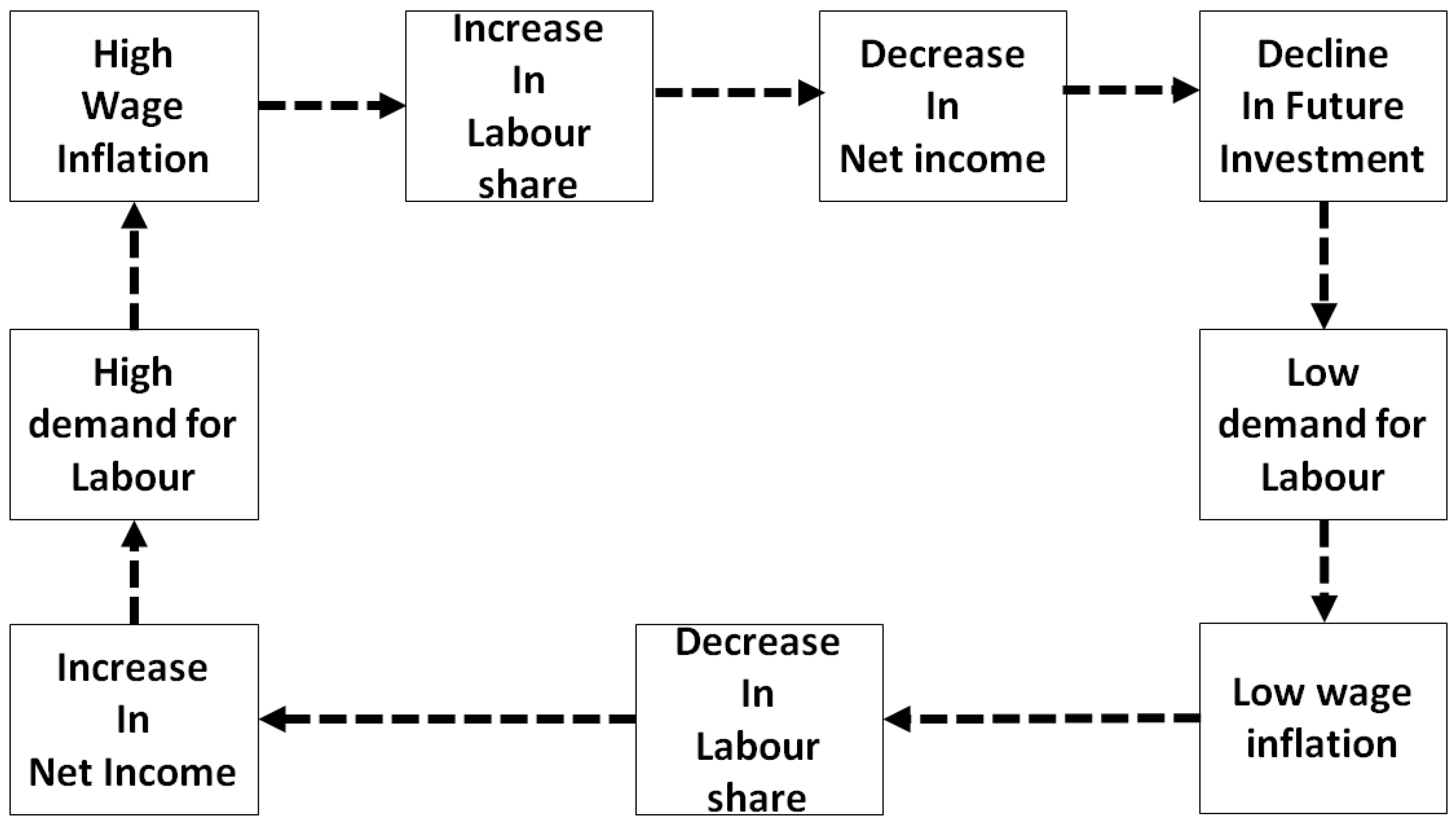Central to this analysis is the Phillips Curve [2,3,4], which describes the inverse relationship between unemployment and wage inflation. A tight labor market, characterized by low unemployment, intensifies competition for workers, driving wages upward. Conversely, high unemployment weakens workers’ bargaining power, suppressing wage growth. This framework provides a basis for evaluating labor market fluctuations and policy interventions. This cyclic behavior is illustrated in Figure 1:

However, the wage growth–employment rate nexus is not solely determined by this inverse relationship. Several factors can either amplify or attenuate the dynamics between these two variables. Inflation and inflation expectations play a crucial role. If both workers and employers anticipate higher inflation, they may demand larger wage increases to preserve their real incomes [5]. This can lead to a situation where wage growth outpaces employment growth, potentially contributing to a broader inflationary spiral. Productivity and skill mismatches further complicate matters. When workers possess skills that align with the demands of the job market, they are more likely to command higher wages [6]. However, structural issues, such as a mismatch between the skills of job seekers and the skills demanded by employers, can lead to persistently high unemployment rates, even in the presence of wage growth in certain sectors [7]. Economic cycles also influence this relationship. During economic booms, employers may struggle to find workers with the required skills, thereby driving wage growth. Conversely, during economic downturns, high unemployment rates can exert downward pressure on wages [8,9]. Additionally, long-term structural changes, such as technological advancements and shifts in industry composition, can profoundly affect the dynamics between wage growth and employment.

Government policies introduce another layer of complexity. Minimum wage laws, labor market regulations, and monetary policies can either augment or mitigate the interplay between wage growth and employment [10]. Policies promoting labor market flexibility may foster employment but potentially restrain wage growth, while minimum wage hikes can bolster wages but may have repercussions on employment levels, particularly for low-skilled workers. Globalization and outsourcing are external factors that further shape this relationship. International trade and outsourcing can lead to wage stagnation in certain industries while simultaneously creating job opportunities in others [11]. The pressures of global competition may suppress wages in sectors exposed to international markets.

The competitive relationship between wage growth rates and employment rates is ever-evolving [12,13]. It is influenced by an intricate web of economic, policy, and structural factors. This relationship is not static and can fluctuate across different economic conditions and over time. As such, policymakers, economists, and businesses continually monitor these dynamics to gauge labor market health and to formulate informed decisions concerning economic policy and workforce development. Recognizing the complex nature of this relationship is essential for promoting both economic stability and the well-being of workers in today’s complex and interconnected world.

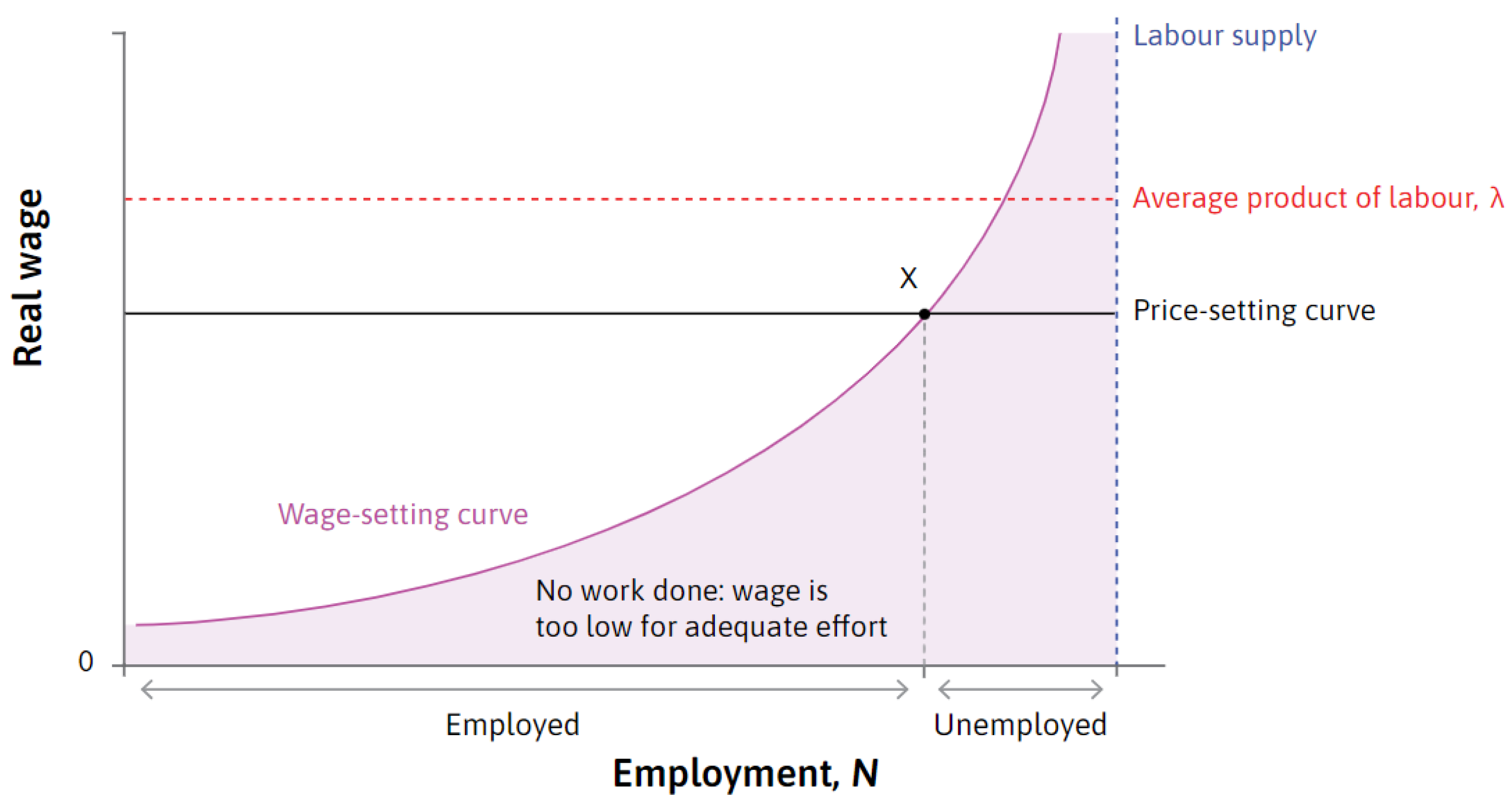
The curve in Figure 2, extracted from [14], underscores the relevance of this study. The shaded region below the wage-setting curve represents labor market conditions where the real wage fails to incentivize work, leading to zero employment and firm profits. A sustained real wage below this threshold results in a labor market collapse, rendering these points infeasible. Labor market equilibrium emerges at the intersection of the wage- and price-setting curves, constituting a Nash equilibrium where firms and workers optimize their decisions in response to each other. At this point, firms set nominal wages where the isocost curve is tangent to the best response function and simultaneously determine the profit-maximizing price. This intersection, denoted as point X, represents the labor market’s Nash equilibrium.

In this study, we propose an extended Goodwin model to investigate wage and employment dynamics in South Africa from 2000 to 2024. Given the pressing challenges of unemployment and wage disparity in developing economies, the original Goodwin framework falls short, as it does not account for real-world institutional and policy interventions. Our model builds upon the classical Goodwin [15] model by integrating a government employment intervention term ($\delta$) and a wage share ceiling ($w_{max}$). The central objective of this research is to evaluate the applicability of this extended model to the South African labor market, where structural rigidities and policy interventions are known to disrupt the endogenous cycles predicted by the classical model.

We employ quantitative methods to analyze the relationship between wage growth and employment dynamics in South Africa. Quantile regression assesses how employment fluctuations influence wages across income levels, providing insight into wage sensitivity [16,17,18]. A moving average technique smooths short-term fluctuations, facilitating the identification of long-term labor market trends and cycles [19,20,21]. The mean absolute error (MAE) quantifies deviations between actual wages and an optimal cyclical wage trajectory, measuring the average discrepancy over time [22,23]. Mathematical analysis of the extended Goodwin model verifies positivity and boundedness, complemented by predictive simulations and phase plane analysis. These methods collectively provide a structured assessment of wage–employment dynamics and their underlying mechanisms.

2. Goodwin’s Growth Cycle Model

The model describes the cyclical interaction between employment and income distribution in a capitalist economy, capturing the dynamic struggle between workers and capitalists. It consists of two coupled differential equations that govern the evolution of the employment rate and the wage share. The employment rate, denoted by u, represents the proportion of the labor force that is employed. Its dynamics depend on the output growth rate g, which drives job creation, and the wage share w, which influences firms’ hiring decisions. The parameter $\alpha$ captures the responsiveness of employment to wage growth, reflecting the extent to which rising labor costs reduce firms’ ability to hire. The wage share, denoted by w, represents the fraction of total output distributed as wages. Its evolution is driven by workers’ bargaining power, represented by $\beta$, which enhances wage growth when employment is high, and the wage growth threshold $\gamma$, which accounts for structural factors limiting wage increases. The system governing the employment rate and wage share is given by:

$$\begin{array}{cc}\hfill {\displaystyle \frac{du}{dt}}& =u(g-\alpha w),\hfill \\ \hfill {\displaystyle \frac{dw}{dt}}& =w(\beta u-\gamma ),\hfill \end{array}$$

(1)

where $g,\alpha ,\beta ,\gamma >0$. Wage share and employment rate are viewed as positive indicators because they reflect the overall health and stability of an economy. Thus, it is necessary to prove that these state variables are positive for all $t\ge 0,$ given positive initial conditions. It is trivial to prove that for initial conditions $u\left(0\right)=u_0,w\left(0\right)=w_0>0,$ the solutions $u\left(t\right)$ and $w\left(t\right)$ are positive for all $t\ge 0.$ Concerning steady states, we first obtain the trivial steady state $E_0=(0,0),$ indicating the state of no employment and no wage share. This steady state exists for all u and w, and it has the eigenvalues ${\lambda }_1=g$ and ${\lambda }_2=-\gamma .$ We have the following proposition on local stability of the trivial steady state.

Proposition 1. 

The trivial steady state $E_0$ is always locally asymptotically unstable since one of the eigenvalues is positive.

We also obtain the non-trivial steady state $E_1=\left({\displaystyle \frac{\gamma }{\beta }},{\displaystyle \frac{g}{\alpha }}\right).$ This steady state exists for all u and w, and it has the eigenvalues ${\lambda }_3=\sqrt{g\gamma }i$ and ${\lambda }_4=-\sqrt{g\gamma }i.$ We note that ${\lambda }_3$ and ${\lambda }_4$ are of opposite signs and are complex conjugate pair with zero real parts; this means that the steady state $E_1$ is a center. We have the following proposition on stability of the non-trivial steady state.

Proposition 2. 

The non-trivial steady state $E_1$ exists for all initial values $u\left(0\right)$ and $w\left(0\right)$ but it is not asymptotically stable.

2.1. The Extended Goodwin Model with Policy Interventions

Following the framework established in [15], we consider a cyclical growth model that captures the interaction between capitalists and workers in a dynamic economic system. The model describes the evolution of the employment rate and wage share, incorporating regulatory constraints such as a capped wage share and government intervention in employment. We let $u\left(t\right)$ represent the employment rate at any time $t\ge 0$, g is the output growth rate, $w\left(t\right)$ is the wage share, $\alpha$ captures the responsiveness of employment to wage growth, and $\delta$ represents government intervention aimed at stabilizing employment. The term $\delta (1-u)$ introduces an exogenous adjustment to employment, where higher intervention occurs when unemployment is high, and the effect diminishes as full employment is approached. This mechanism aligns with Phillips curve dynamics, where inflationary pressures may emerge as unemployment decreases. We have that $\beta$ represents workers’ bargaining power, $\gamma$ is the wage growth threshold, and $w_{max}$ denotes an upper bound on the wage share imposed by economic or policy constraints. The term $\left(1-{\displaystyle \frac{w}{w_{max}}}\right)$ ensures that wage growth slows as w approaches its maximum permissible value, thereby preventing excessive wage expansion that could destabilize capital accumulation. In line with the Phillips curve, higher employment rates exert upward pressure on wage share through wage inflation, reinforcing the cyclical nature of wage and employment fluctuations in the model. The employment rate and wage share evolve according to the system:

$$\begin{array}{c}{\displaystyle \frac{du}{dt}}=u(g-\alpha w)+\delta (1-u),\hfill \\ {\displaystyle \frac{dw}{dt}}=w(\beta u-\gamma )\left(1-{\displaystyle \frac{w}{w_{max}}}\right),\hfill \end{array}$$

(2)

where we assume that all parameters $g,\delta ,\alpha ,\beta ,\gamma ,$ and $w_{max}$ are non-negative. It can be shown that the system has positive and bounded solutions. We obtain the steady states:

$$\left\{E_2=\left({\displaystyle \frac{\gamma }{\beta }},{\displaystyle \frac{g\gamma +\beta \delta -\gamma \delta }{\alpha \gamma }}\right),E_3=\left({\displaystyle \frac{\delta }{-g+\delta }},0\right),E_4=\left({\displaystyle \frac{\delta }{-g+w_{max}\alpha +\delta }},w_{max}\right)\right\},$$

which all exist if $\delta \ge g$. We present the stability analysis of the steady states in

Table 1. Summary of stability conditions for each steady state.

Steady State	Stability Conditions
$\left({\displaystyle \frac{\gamma }{\beta }},{\displaystyle \frac{g\gamma +\beta \delta -\gamma \delta }{\alpha \gamma }}\right)$	${\mathrm{\Delta }}_1\le 0$    or    ${\mathrm{\Delta }}_1<\beta \delta \sqrt{w_{max}\alpha }$
$\left({\displaystyle \frac{\delta }{-g+\delta }},0\right)$	$g<\delta$    and    $\beta -\gamma <-{\displaystyle \frac{g\beta }{-g+\delta }}$
$\left({\displaystyle \frac{\delta }{-g+w_{max}\alpha +\delta }},w_{max}\right)$	$g<w_{max}\alpha +\delta$    and    $\gamma <-{\displaystyle \frac{\beta \delta }{g-w_{max}\alpha -\delta }}$

:

• where

$${\mathrm{\Delta }}_1=4g(g-w_{max}\alpha ){\gamma }^3+4(-2g+w_{max}\alpha ){\gamma }^2(-\beta +\gamma )\delta +\left(w_{max}\alpha {\beta }^2+4{(\beta -\gamma )}^2\gamma \right){\delta }^2.$$

The steady states represent equilibrium points where employment and wage share remain constant over time. Their stability depends on the interaction between wage dynamics, government intervention, and output growth. The first steady state balances wage growth and employment fluctuations, with stability determined by the discriminant ${\mathrm{\Delta }}_1$. The second steady state corresponds to a wage collapse, requiring low output growth and restricted bargaining power for stability. The third steady state occurs when wages reach their upper bound, with stability contingent on sufficient government intervention and wage responsiveness. Overall, stability is influenced by the balance between employment growth and wage dynamics, highlighting the risks of both excessive wage suppression and uncontrolled wage expansion.

2.2. Simulation of the Ideal Model

We explore the dynamics of an extended Goodwin model using simulations to demonstrate the ideal implications of the model by considering their coupled evolution, incorporating a capped wage share ($w_{max}$) and government employment intervention ($\delta$). To ensure reproducibility and clarity, we explicitly outline the simulation setup: the model is solved numerically using a standard Runge–Kutta integration scheme with fixed step size, over a horizon of 200 periods. Initial conditions are set to $u=0.8$ for the employment rate and $w=0.4$ for the wage share.

We use illustrative parameter values, guided by the literature on Goodwin-type models and stylized macroeconomic behavior: output growth rate ($g=0.36$), employment responsiveness to wages ($\alpha =0.89$), intervention strength ($\delta =0.02$), workers’ bargaining power ($\beta =0.55$), wage growth threshold ($\gamma =0.29$), and maximum wage share ($w_{max}=0.68$). The output growth rate g is set at a moderate level to capture long-run productivity-driven expansion, while $\alpha$ is chosen relatively high to reflect the sensitivity of employment to wage dynamics in developing economies. The intervention parameter $\delta$ is small but positive, representing limited but non-negligible government employment support. The bargaining power $\beta$ and wage growth threshold $\gamma$ are calibrated to ensure realistic wage–employment cycles, with $\beta$ slightly above 0.5 to capture worker influence without implying dominance. Finally, $w_{max}$ is set below unity to represent the realistic ceiling on labor’s share of income in a capitalist economy. These values are not empirical estimates, but rather plausible stylized settings that allow us to demonstrate the cyclical and stabilizing features of the model. Together, these parameters influence both the amplitude and persistence of cycles: higher $\alpha$ increases volatility in employment, while stronger intervention $\delta$ accelerates convergence to equilibrium. Results are visualized in time series and phase plane plots.

The phase plane diagram in Figure 3 illustrates the cyclical relationship between employment rates and wage share in a capitalist economy (see also [24]). It shows four economic phases: Depression (low employment and wage share), Recession (declining employment and wage share), Boom (rising employment and wage share), and Recovery (improving employment and wage share). Arrows indicate the transitions between these phases, highlighting the interdependence of employment dynamics and income distribution. The diagram reflects the predator–prey model by Goodwin, where the growth rates of wages and employment are closely linked to broader economic fluctuations. In this extended formulation, the oscillations are not perpetual but damped, indicating convergence toward equilibrium rather than indefinite cycles.

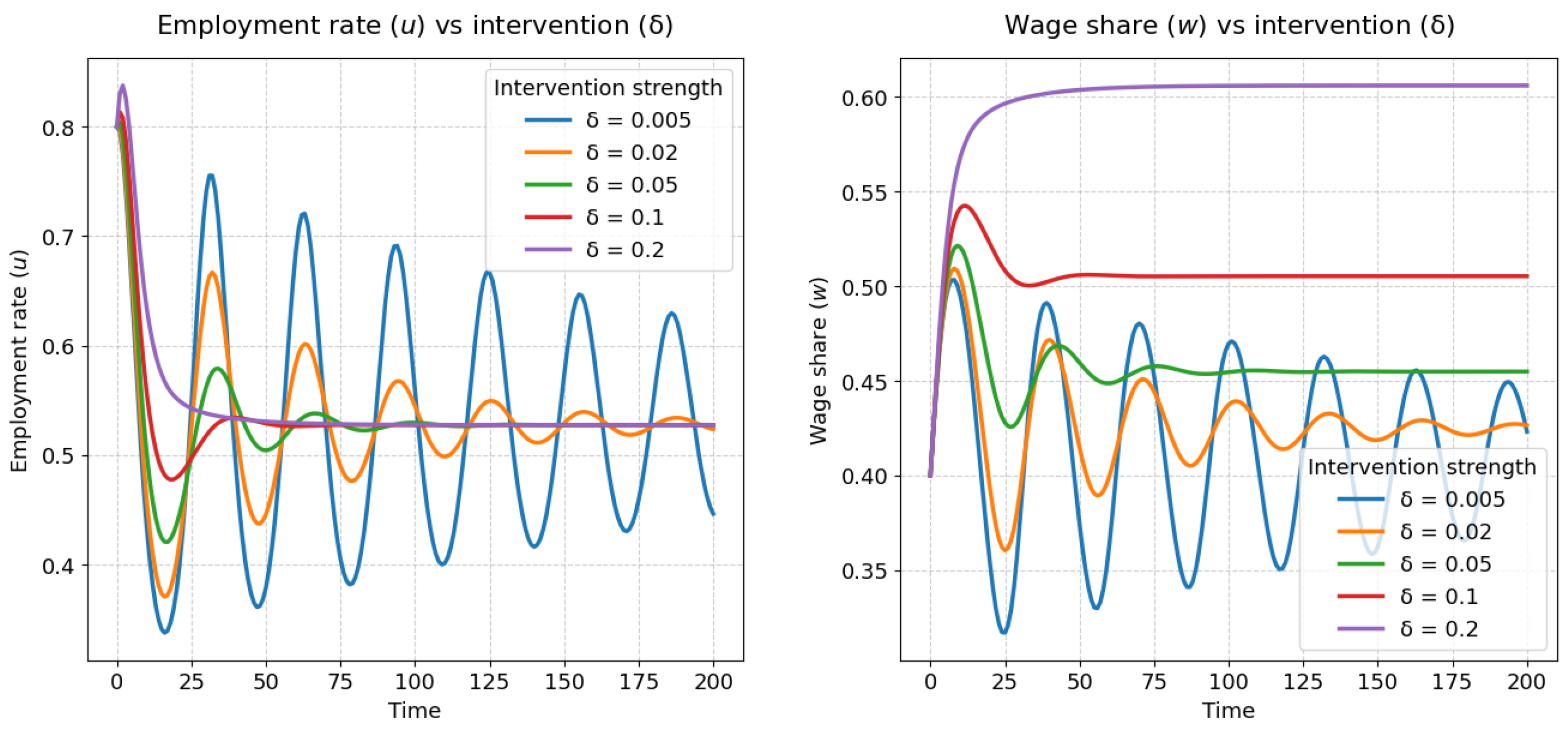
The simulation results, presented in Figure 4, depict the joint time-series evolution of the employment rate (u) and the wage share (w). The trajectories reveal the characteristic cyclical interaction predicted by the Goodwin framework, whereby fluctuations in employment precede corresponding adjustments in the wage share. Consistent with the predator–prey structure of the model, peaks in employment are followed by increases in wage share, while declines in employment lead to reductions in wages. Importantly, the extended formulation introduces additional stabilizing mechanisms: the incorporation of a wage-share ceiling ($w_{max}$) and government intervention ($\delta$) results in damped oscillations, such that the amplitude of cycles diminishes over time. Rather than exhibiting persistent closed cycles, the system converges toward a stable equilibrium, thereby illustrating how these extensions mitigate perpetual fluctuations and promote long-run stability.

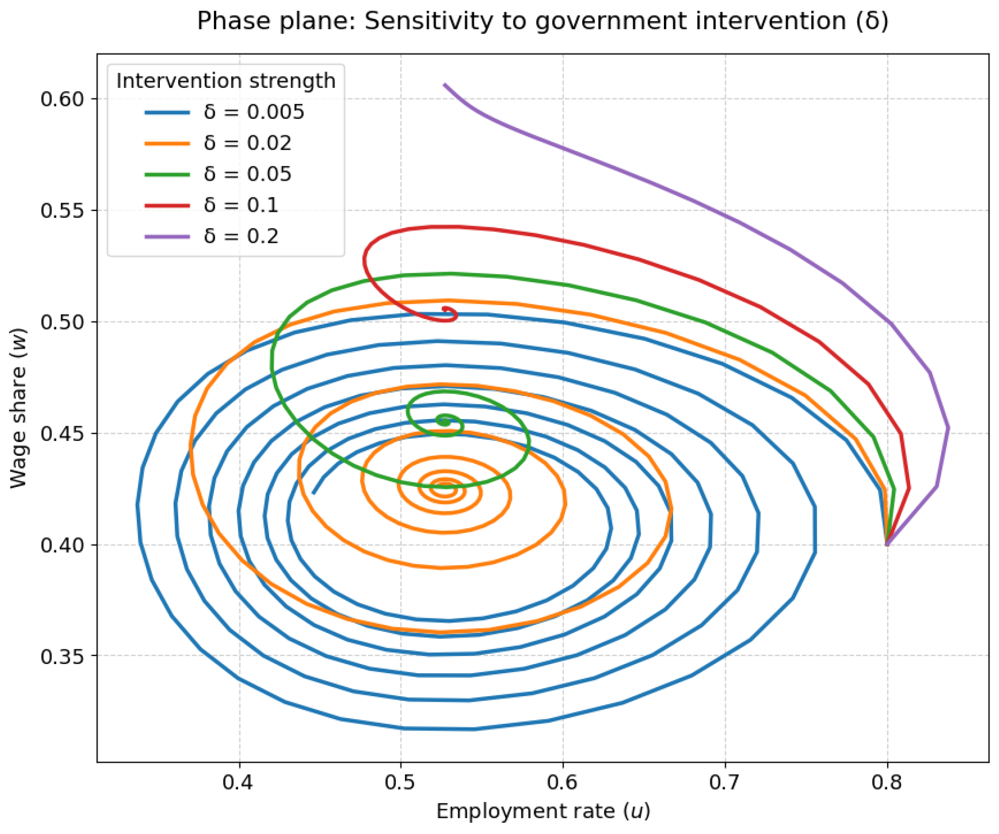
The phase plane diagram provides a holistic view of these dynamics. All trajectories begin from the same initial condition ($u=0.8$, $w=0.4$) and spiral toward the steady-state equilibrium. The extent of spiraling reflects the amplitude and persistence of cycles. With weak intervention ($\delta =0.005$), the spiral is wide and persistent, reflecting slow convergence. As $\delta$ increases, the spirals tighten and shorten, showing faster stabilization. At $\delta =0.2$, the path is almost a straight line to equilibrium, with no discernible cycles. Together, these results demonstrate that government intervention plays a stabilizing role in the Goodwin framework: it suppresses endogenous cycles and promotes faster convergence to a steady-state configuration of employment and wage share.

2.3. Sensitivity to Government Intervention

Figure 5 contains two time-series plots that illustrate how the employment rate (u) and wage share (w) evolve over time, with each colored line representing a different level of government intervention strength ($\delta$). In the left plot, which shows the employment rate, all trajectories begin at the same initial value ($u=0.8$) and subsequently display a cyclical, oscillatory behavior that dampens as time progresses. As the intervention strength $\delta$ increases, the oscillations dampen more rapidly and the system converges to its stable steady-state equilibrium in a shorter period. For the lowest intervention level ($\delta =0.005$, represented by the blue line), the cycles are large in amplitude and persist for a long duration. When $\delta$ is increased to $0.05$ (green line) and $0.1$ (red line), the oscillations diminish in amplitude more quickly. At the highest intervention strength ($\delta =0.2$, purple line), the employment rate exhibits almost no oscillation, settling rapidly to its equilibrium value.

The right plot in Figure 5 shows the trajectories of the wage share, where a similar pattern emerges. The wage share exhibits damped oscillations, and the rate at which these oscillations disappear is positively correlated with the value of $\delta$. At the weakest intervention level, the wage share cycles persist between high and low values over an extended period. At the strongest intervention level, the wage share increases rapidly from its initial value to its equilibrium without any noticeable oscillation. This indicates that government intervention functions as a stabilizing mechanism for both employment and wages.

Figure 6 presents a phase plane diagram combining the trajectories of the employment rate and wage share for different values of $\delta$. All trajectories start from the same initial condition ($u=0.8,w=0.4$) and spiral inward toward the non-trivial steady-state equilibrium, confirming the damped oscillatory behavior observed in the time-series plots. The extent of spiraling reflects the speed of convergence: for the lowest intervention ($\delta =0.005$, blue line), the trajectory circles many times before stabilizing, while higher values of $\delta$ produce tighter and shorter spirals. At the strongest intervention ($\delta =0.2$, purple line), the trajectory moves almost directly to equilibrium, with no visible oscillations.

2.4. Tornado Plot Analysis

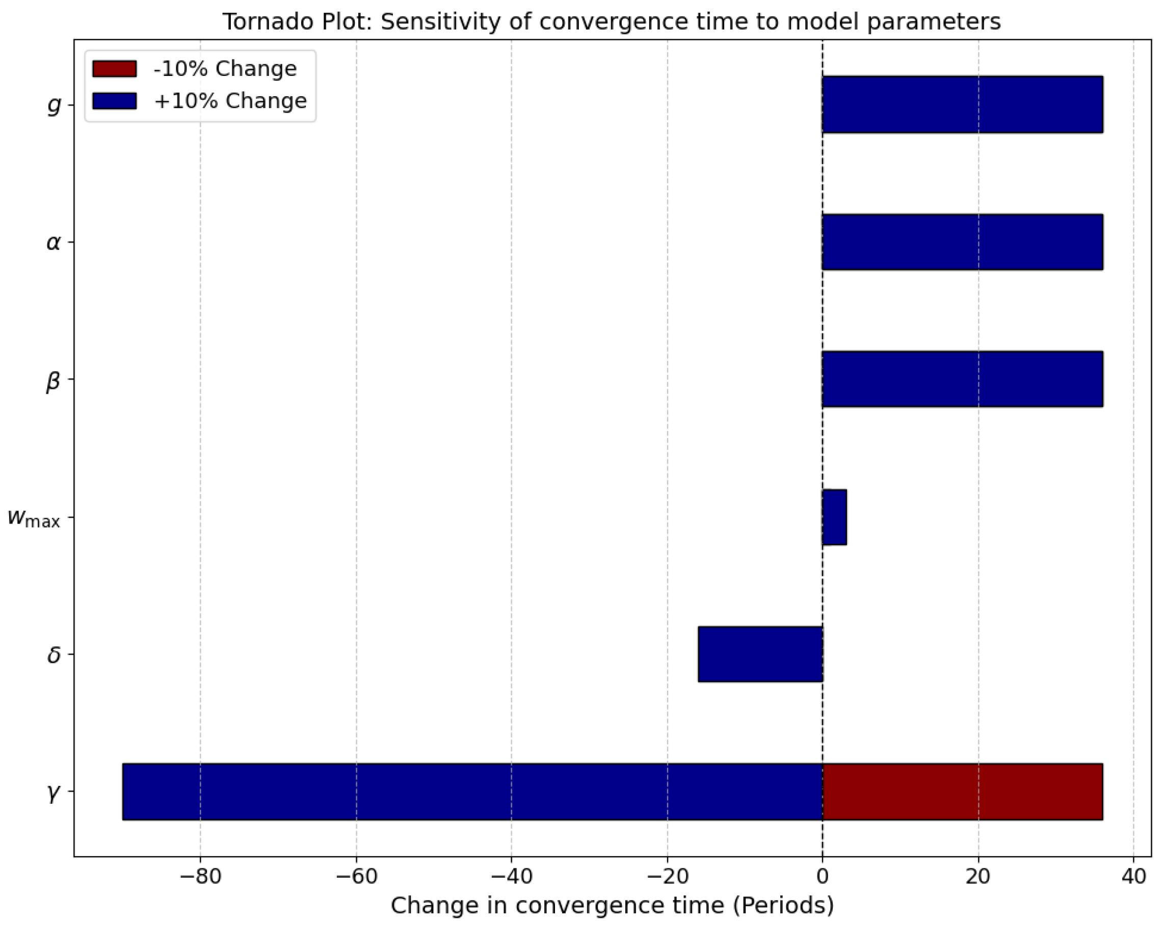
The tornado plot in Figure 7 provides a visual representation of the sensitivity of the model’s convergence time to variations in key parameters. Each horizontal bar corresponds to a single model parameter and shows the effect of a $\pm 10\%$ deviation from its baseline value. The parameters are ordered from the most to the least influential, allowing a clear comparison of their relative impact on the speed at which the system reaches its steady-state equilibrium.

Analysis of the plot reveals that the parameter with the strongest effect is $\gamma$ (wage growth threshold). A reduction in $\gamma$ shortens the convergence time considerably, while an increase prolongs it. This behavior indicates that the threshold for wage growth plays a central role in determining the speed at which cyclical fluctuations in employment and wage share dampen, making it a critical factor in the stabilization of economic cycles.

The next most influential parameters are $\beta$ (workers’ bargaining power) and $\alpha$ (responsiveness of employment to wage growth). Variations in either of these parameters produce substantial changes in convergence time, reflecting the strong interdependence between labor market dynamics and the wage–employment feedback mechanisms embedded in the model. Higher bargaining power or higher responsiveness amplifies the sensitivity of the system, thereby influencing how quickly equilibrium is restored.

Parameters g (output growth rate) and $\delta$ (government intervention) exhibit a moderate effect on convergence dynamics. An increase in government intervention, $\delta$, reduces the convergence time, consistent with earlier observations from the time-series analysis that higher intervention accelerates stabilization. While these parameters are important for overall dynamics, their influence is less pronounced than that of $\gamma$, $\beta$, or $\alpha$, suggesting that internal labor market mechanisms dominate the speed of convergence.

The least influential parameter is $w_{max}$ (maximum wage share). Adjusting $w_{max}$ by $\pm 10\%$ produces only minor changes in convergence time, implying that the upper bound on wage share is not a limiting factor for the damping of cycles within the simulated parameter ranges.

Overall, the tornado plot clearly demonstrates that $\gamma$, $\beta$, and $\alpha$ are the dominant drivers of convergence dynamics in the extended Goodwin model. The plot also confirms that government intervention, while stabilizing, does not override the effects of internal labor market parameters. These insights are critical for understanding which aspects of the model most strongly influence the system’s behavior and can guide both theoretical exploration and policy-oriented simulations in the context of developing economies.

3. Evidence in the South African Context

In examining South Africa’s labor–wage dynamics, we provide evidence that there are no obvious cycles as depicted by the Goodwin’s model. We use quantile regression to establish how the relationship between employment and wages varies across different segments of the workforce from 2000–2024 using wage rate and employment rate data from World Bank data and the Federal Reserve Bank of St Louis [25,26]. We explore how wage growth is influenced by employment fluctuations at various income levels, uncovering asymmetries in the wage–employment relationship. This approach highlights the unique challenges and dynamics within South Africa’s labor market, particularly in terms of economic cycles and income distribution. These dynamics provide the framework for assessing their relevance in a developing economy such as South Africa. The South African case serves as an illustrative application, allowing us to examine whether the stylized cyclical mechanisms of the Goodwin model align with the country’s socio-economic conditions and observed data patterns.

3.1. Quantile Regression on Wage–Labor Dynamics

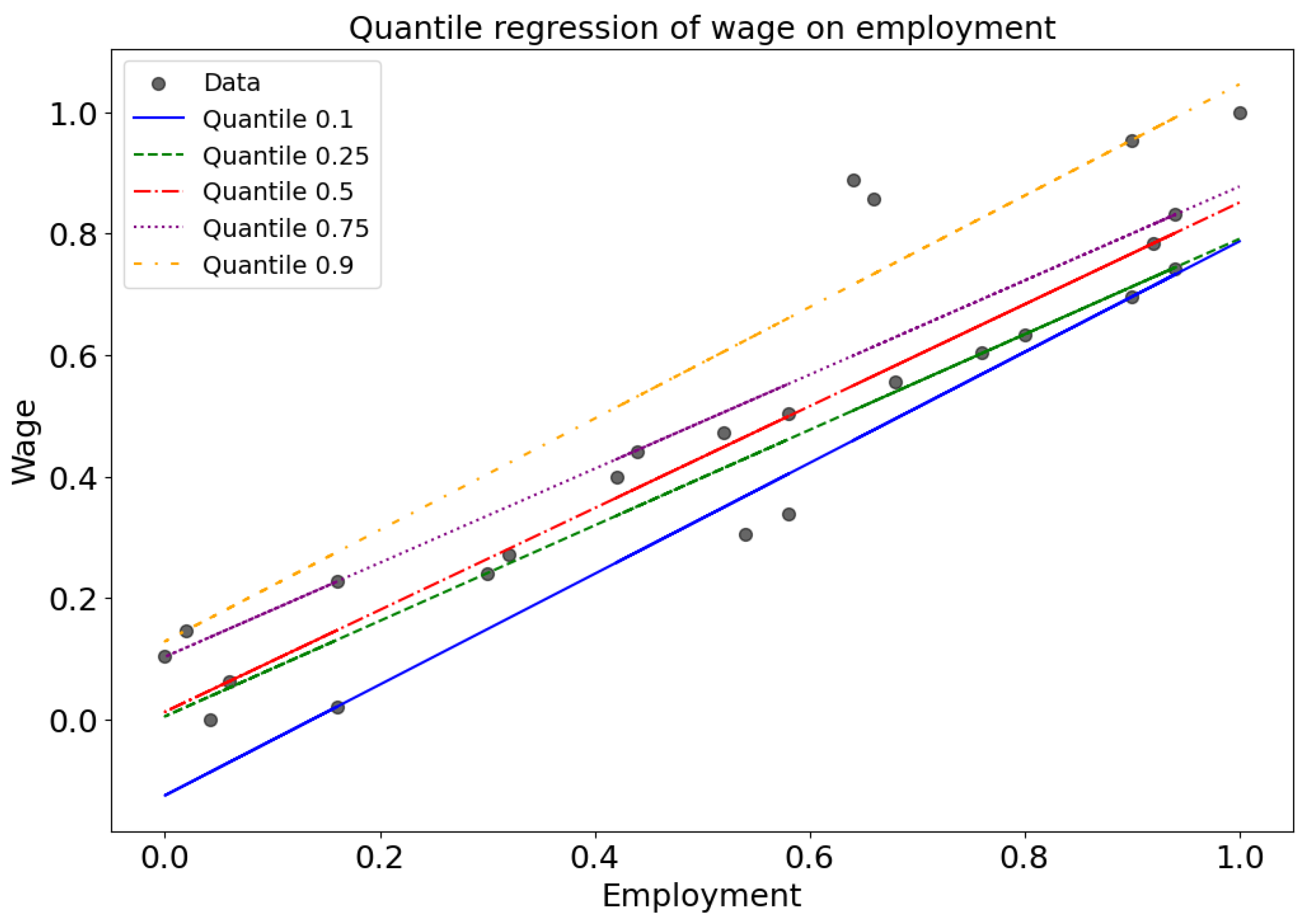
Quantile regression reveals that the relationship between employment and wages varies across different wage quantiles. At lower quantiles, the effect of employment on wages is weaker, while at higher quantiles, the impact is stronger.

This pattern does not fully align with Goodwin’s cyclical model. There are instances of rising employment driving wage growth until it exceeds productivity, reducing profitability and triggering recession. Recovery follows as low wages restore profits, increasing employment. However, the wage data does not display the desired responsiveness to the employment cycles, and the effect is stronger as wages increased in the later years in general, reflecting wage–employment asymmetry. At the $0.1$ and $0.25$ quantiles (see Figure 8), wage growth rate is highly sensitive to fluctuations in employment rate, indicating that initially, the wages were responsive to changes in labor market conditions. At the $0.75$ and $0.9$ quantiles (see Figure 8), the wage–employment relationship remains strong, suggesting that high wage rates benefit from tight labor markets. In general, the growth rates of wages and employment diverge across quantiles, reflecting a non-uniform growth trajectory.

3.2. Wage Mismatch and Intervention Metrics in South Africa

We use the moving average to smooth short-term fluctuations, revealing long-term trends and cycles. By reducing noise, it allows us to observe underlying patterns and highlight periods of growth or decline and economic phases, such as booms and recessions. The graphs in Figure 9 show the cyclical analysis of employment and wages. The employment subgraph reveals an upward trend, with distinct peaks (green triangles) and troughs (red triangles), indicating fluctuations corresponding to economic cycles. In contrast, the wage subgraph shows a steady increase without visible peaks or troughs, indicating a stable economic environment for wages, with gradual increases rather than large fluctuations. Thus, employment shows cyclical behavior, and wages appear less sensitive to economic cycles. This contradicts the Goodwin’s growth cycle model.

To affirm our observations, we further analyze raw wage data to determine the mismatches. We start by defining a smooth, upward-sloping wage trend as a linear function:

$$w_{\mathrm{original}}=0.0417t-0.0178$$

where t is time, and the wage grows at a constant rate of $0.0417$ per unit of time. To model cyclical wage behavior, without loss of generality, we introduce periodic fluctuations with amplitude $A=0.1$ (determines the strength of the cycles) and frequency $B=0.5$ (controls how often cycles occur over time). We selected A and B based on employment cycle trends observed in the wages dataset. The amplitude is small enough to preserve the overall wage trajectory but introduces oscillations that reflect ideal cyclical behavior, leading to an “ideal” wage function:

$$w_{\mathrm{ideal}}=w_{\mathrm{original}}+Asin\left(Bt\right)$$

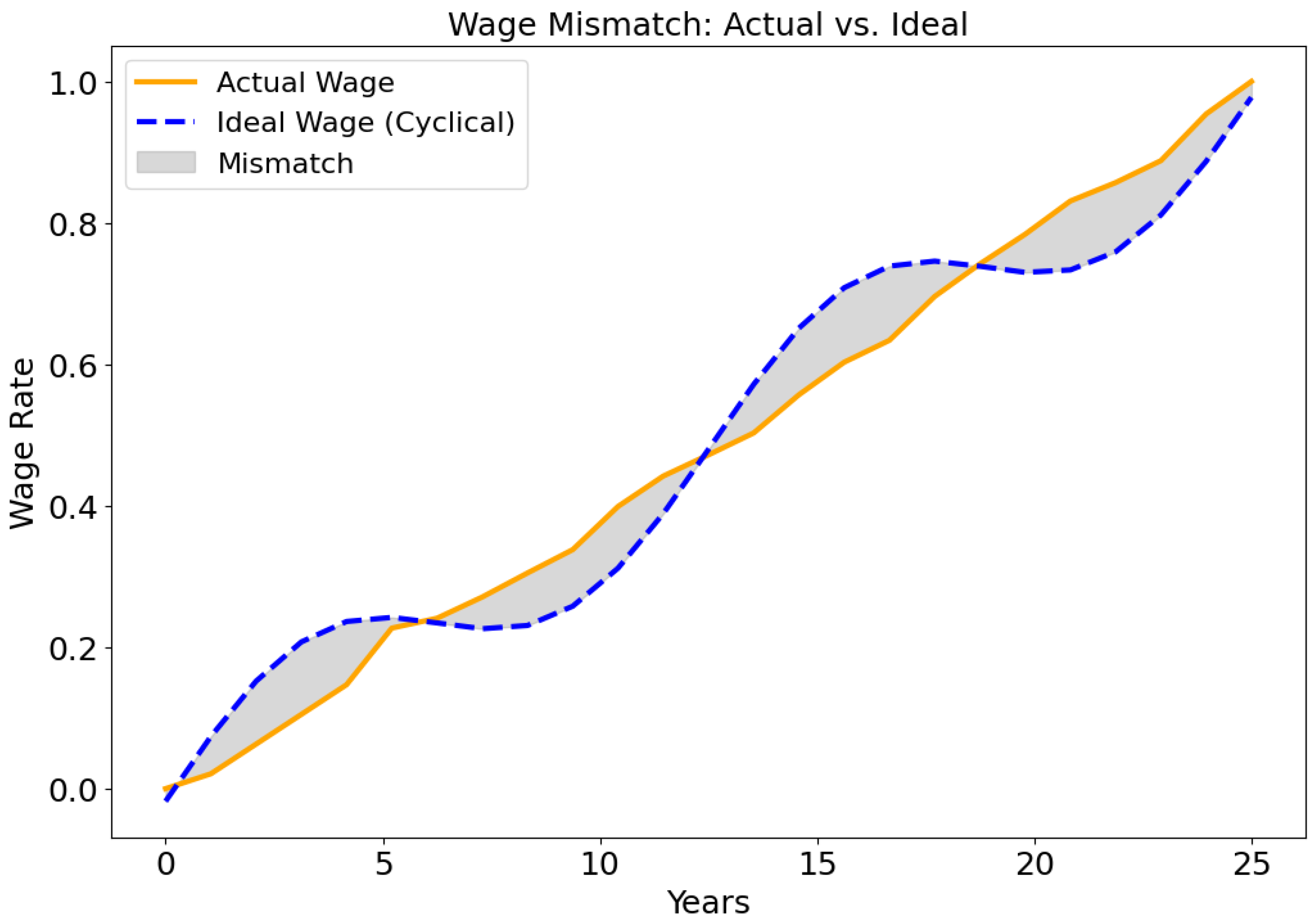
The wage mismatch graph in Figure 10 offers a reflection of how ideal and actual wages differ over time. The x-axis starts from the year 2000 until 2024 (25 years), reflecting a long-term perspective, while the y-axis measures the magnitude of the mismatch, reaching values as high as $0.14$ indicating significant discrepancies in certain periods. Notably, the most pronounced mismatches appear around the year 2012 and between the years 2019 and 2024, suggesting substantial deviations during these intervals. In contrast, the periods from 2005 to 2009 and from 2015 to 2019 show relatively lower mismatches, implying a closer alignment between ideal and actual wages. Overall, the graph reveals that wage mismatches fluctuate considerably over time, potentially in response to economic events or shifts in labor market conditions.

This mismatch reflects how actual wages deviate from the ideal cyclical trajectory due to economic factors as shown in Figure 10. We compute the wage mismatch as the absolute difference between the ideal and original wages:

$$w_{\mathrm{mismatch}}=|w_{\mathrm{ideal}}-w_{\mathrm{original}}|.$$

The gray area is effectively the absolute difference between the original wage trend $w\left(t\right)$ and the idealized cyclical wage $w^{*}\left(t\right)$:

$$\mathrm{\Delta }w\left(t\right)=\left|w^{*}\left(t\right)-w\left(t\right)\right|.$$

The total area under the curve can be integrated over time to measure the cumulative wage mismatch:

$${\int }_0^{t_f}\left|w^{*}\left(t\right)-w\left(t\right)\right|dt.$$

This integral provides a measure of how much real wages deviate from the theoretically optimal response. To quantify how much the adjusted wage deviates from the original, we compute:

$$MAE={\displaystyle \frac{1}{N}}\sum _{i=1}^N\left|w^{*}\left(t_i\right)-w\left(t_i\right)\right|$$

where N is the number of time points. A relatively low MAE ($0.0639$) indicates that the modifications are minor but sufficient to introduce cyclicality.

The cumulative mismatch in this simulation is $1.6071$, a significant numerical metric that represents the total deviation between the actual and ideal wage trajectories over the observed period. This mismatch reflects the degree to which market forces or policy interventions fail to align actual wage adjustments with the expected cyclical patterns.

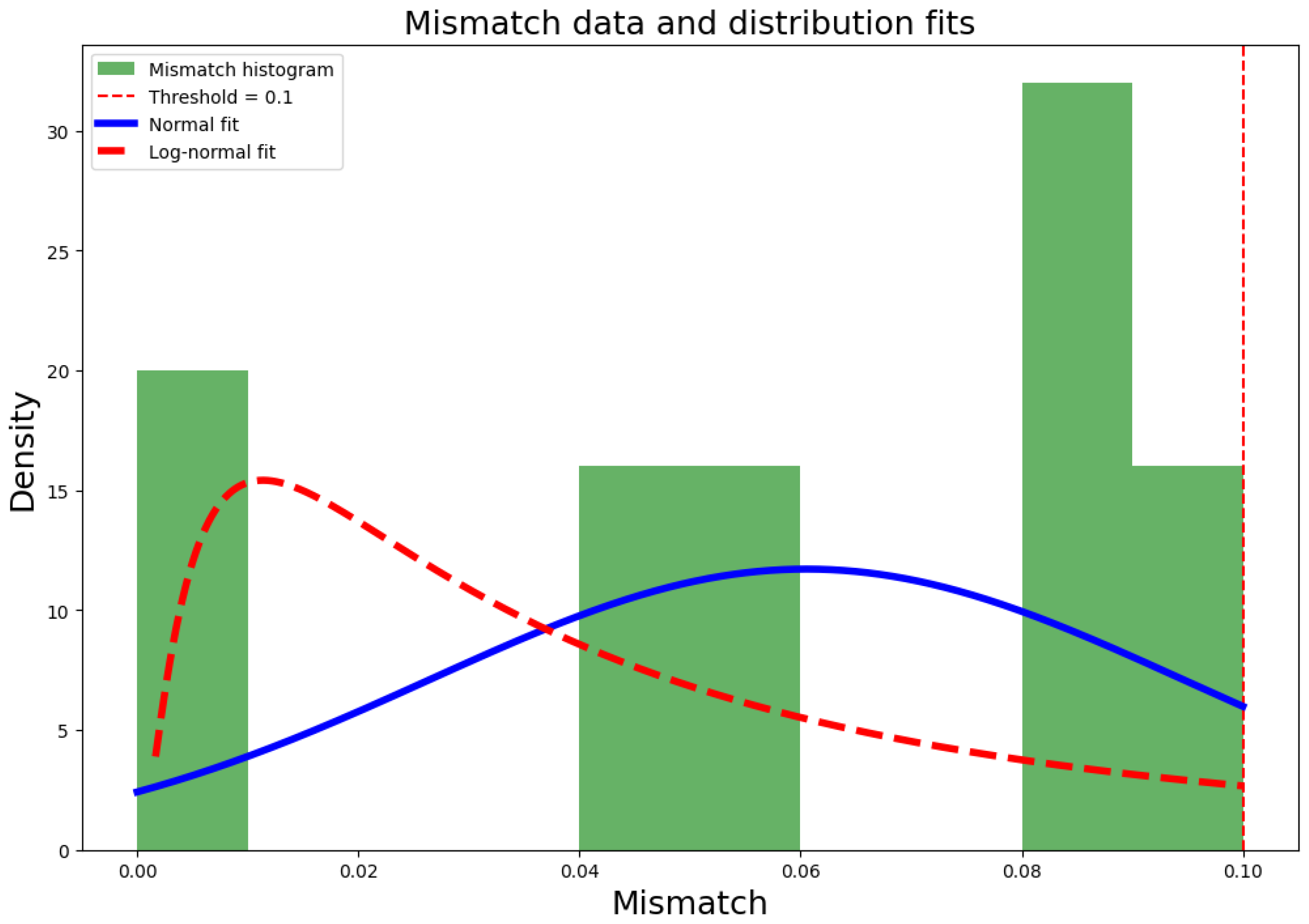
Figure 11 shows a histogram displaying the distribution of the absolute wage mismatch, with the green bars representing the observed frequency of mismatch values.

The blue curve (solid line) shows the fit of a half-normal distribution, and the red curve (dashed line) shows the fit of a log-normal distribution. Because the mismatch is defined as the absolute deviation $\mathrm{\Delta }w\left(t\right)= |w^{*}\left(t\right)-w\left(t\right)|$, it cannot be mean-zero normal. If the underlying signed error $Z\left(t\right)=w^{*}\left(t\right)-w\left(t\right)$ is Gaussian with variance ${\sigma }^2$, then the mismatch follows a half-normal distribution:

$$\mathrm{\Delta }w\left(t\right)\sim \mathrm{HalfNormal}\left(\sigma \right).$$

The exceedance probability for a policy threshold T is then given by

$$P(\mathrm{\Delta }w\left(t\right)>T)=2\left[1-\mathrm{\Phi }\left(\frac{T}{\sigma }\right)\right],$$

where $\mathrm{\Phi }$ is the standard normal cumulative distribution function.

Since this probability is constant over time, integrating over $[0,t_f]$ simplifies to:

$$P{(\mathrm{\Delta }w\left(t\right)>T)}_{\mathrm{total}}=2\left[1-\mathrm{\Phi }\left(\frac{T}{\sigma }\right)\right]$$

Thus, the total probability matches the single-time probability. Using the reported MAE of $0.0639$, we estimate $\sigma \approx 0.0801$. For the threshold $T=0.1$, the exceedance probability is approximately $0.212$, i.e., there is about a $21\%$ chance that the mismatch exceeds the policy limit.

This adjustment preserves the graphical results but ensures the statistical interpretation matches the nonnegative definition of mismatch.

4. Discussion and Conclusions

This study evaluates the applicability of the extended Goodwin model with policy interventions in South Africa’s labor market from 2000 to 2024. The model predicts cyclical employment and wage share dynamics, incorporating a capped wage share and government intervention. Simulations generate cyclical patterns, but empirical analysis, including quantile regression and wage mismatch evaluation, reveals significant deviations from the predicted cycles. Quantile regression results indicate wage sensitivity variations across income levels, while wage mismatch analysis shows substantial discrepancies between observed and ideal cyclical wages, peaking in 2009 and 2019–2024, with a mean absolute error (MAE) of $0.0639$. The Kolmogorov–Smirnov test confirms a half-normal distribution of wage mismatches, suggesting systematic labor market constraints that challenge the Goodwin model’s assumptions.

The Goodwin model predicts cyclical wage–employment interactions driven by profit constraints on wage growth. However, findings indicate that while employment exhibits cyclical behavior, wage dynamics remain relatively stable and display limited responsiveness to labor market fluctuations. This divergence suggests structural labor market rigidities disrupting wage cycles. Quantile regression results show that lower-income groups ($0.1$ and $0.25$ quantiles) experience greater wage sensitivity to employment changes, while higher-income groups ($0.75$ and $0.9$ quantiles) benefit more from tight labor markets, reflecting increased bargaining power. This asymmetry aligns with Marxist conflict theory, indicating that wage growth disproportionately favors those with greater bargaining power.

Wage mismatch analysis further supports deviations from Goodwin’s predicted cycles. Mismatches peak around 2010 and 2019–2024, coinciding with major economic disruptions. Lower mismatches in the periods 2005–2009 and 2015–2019 indicate periods of relative alignment between wages and employment, suggesting that macroeconomic stability allows partial convergence toward ideal cyclical patterns. The mismatch peaks in 2010 likely result from the aftermath of the 2008 financial crisis, high unemployment, and wage stagnation. Similarly, 2019–2024 reflects the impact of COVID-19 (2020–2022), mass layoffs, wage volatility, and inflationary pressures. Other contributing factors include the Great Resignation, accelerated automation, and shifts in labor demand, which intensified wage disparities across sectors. In contrast, periods of lower mismatch indicate greater wage–employment synchronization driven by macroeconomic stability and post-crisis recovery.

Several factors contribute to the deviations from Goodwin’s predicted cycles. Labor market frictions, including skill mismatches and delayed wage adjustments, hinder immediate wage responses to employment shifts. Institutional factors, such as strong labor unions, minimum wage policies, and collective bargaining, reinforce wage rigidity, limiting cyclical fluctuations. Inflation also plays a role; during high-inflation periods, real wages decline even if nominal wages remain stable, further disrupting cyclical patterns. Structural shifts, particularly the transition from manufacturing to services, alter the composition of the labor market, producing long-term adjustments rather than periodic fluctuations. Government interventions, such as wage subsidies and employment support programs, further stabilize income levels, reducing cyclical wage fluctuations. Future analyses could employ difference-in-differences methods to assess the impact of minimum wage adjustments across quantiles, or sector-level fixed effects to evaluate the effects of industrial shifts on wage dynamics. Additionally, a disaggregated analysis by labor type and sector could reveal heterogeneous wage–employment interactions, which may substantially modify aggregate outcomes.

This study concludes that while the extended Goodwin model captures key employment–wage interactions, its prediction of cyclical wage share dynamics does not fully align with South African empirical data. Wage growth is less cyclical and more structurally constrained, with significant deviations from the model’s trajectory. These findings highlight the need to account for institutional, policy-driven, and macroeconomic factors when applying theoretical economic models to real-world labor markets. The definition of an “ideal” cyclical wage pattern critically influences mismatch metrics, and extending the time series could uncover more intricate wage dynamics. Incorporating additional labor market rigidities and sectoral heterogeneity in future research may enhance the applicability of cyclical growth models in developing economies.