Article

Balancing Resolution with Analysis Time for Biodiesel–Diesel Fuel Separations Using GC, PCA, and the Mahalanobis Distance

by
Edward J. Soares
1,*,†,
Alexandra J. Clifford
2,
Carolyn D. Brown
2,
Ryan R. Dean
2 and
Amber M. Hupp
2,*,†
1
Department of Mathematics and Computer Science, College of the Holy Cross, Worcester, MA 01610, USA
2
Department of Chemistry, College of the Holy Cross, Worcester, MA 01610, USA
*
Authors to whom correspondence should be addressed.
These authors contributed equally to this work.
Separations 2019, 6(2), 28; https://doi.org/10.3390/separations6020028
Submission received: 31 March 2019 / Revised: 10 May 2019 / Accepted: 15 May 2019 / Published: 27 May 2019
(This article belongs to the Special Issue Chromatography and Chemometrics)

Abstract

:
In this work, a statistical metric called the Mahalanobis distance (MD) is used to compare gas chromatography separation conditions. In the two-sample case, the MD computes the distance between the means of the multivariate probability distributions of two groups. Two gas chromatography columns of the same polarity but differing length and film thickness were utilized for the analysis of fatty acid methyl esters in biodiesel fuels. Biodiesel feedstock samples representing classes of canola, coconut, flaxseed, palm kernal, safflower, soy, soyabean, sunflower, tallow, and waste grease were used in our experiments. Data sets measured from each column were aligned with the correlated optimized warping (COW) algorithm prior to principal components analysis (PCA). The PC scores were then used to compute the MD. Differences between the data produced by each column were determined by converting the MD to its corresponding p-value using the F-distribution. The combination of COW parameters that maximized the p-value were determined for each feedstock separately. The results demonstrate that chromatograms from each column could be optimally aligned to minimize the MD derived from the PC-transformed data. The corresponding p-values for each feedstock type indicated that the two column conditions could produce data that were not statistically different. As a result, the slight loss of resolution using a faster column may be acceptable based on the application for which the data are used.

1. Introduction

Achieving adequate resolution in complex chromatograms is the most important goal in gas chromatography (GC) [1]. For biodiesel-diesel blended fuels, a long, very polar column is traditionally used to separate the many diesel components as well as to isolate the long chain fatty acid methyl esters (FAMEs) present in biodiesels [2,3,4]. The diesel components elute at low to mid-range temperatures and are often difficult to completely isolate, leading to unresolved baseline humps [5,6]. The alkanes have large, easily recognizable peaks with various aromatic components present in diesel and are interspersed throughout the chromatogram. The long length and high polarity of the column allows for separation of FAME isomers, which generally elute later in the run, as their boiling points are much higher than the diesel components [2]. Overall, the run times tend to be long, on the order of thirty to sixty minutes, and can be longer depending on the length and polarity of the column and the desired separation of the FAME isomers.
While resolution is paramount, analysis time can also be a key factor in selecting column conditions, especially for separations with excess resolution. For laboratories that run many samples each day, a difference in run time of only a few minutes can make a significant impact on the number of total runs that can be performed each day. There are a number of methods to call upon to decrease run time including: increasing the temperature ramp, increasing the carrier gas flow rate, altering the column chemistry, or decreasing the column length and film thickness [1,3,7]. The first two methods can be used when resolution far exceeds that needed for separation or when a different column is not available. The latter two methods require a different column be put in place. As an example of alternate column chemistry, Turner et al. [8] used a novel ionic column for the separation of FAME isomers in ruminant tissue. Analysis time was fast (under 12 min) and resulted in good separation of isomers. However, using a different column chemistry can result in swapping of peaks based on polarity [9], and could lead to decreased resolution, which is not ideal for all applications. Alternatively, Masood et al. [10] investigated two columns of the same polarity (DB-FFAP and ZB-FFAP) for the separation of fatty acids found in blood. Resolution of the shorter gas GC column (15 m × 0.1 mm × 0.1 μm) was comparable to a longer, traditional column (30 m × 0.25 mm × 0.25 μm) with a significant decrease in run time (from 45 to 8 min).
The challenge with decreasing GC run time is to not permit decreased resolution. In reality, this can be difficult to achieve. Multivariate curve resolution-alternating least squares (MCR-ALS) has been successful for fast chromatography that leaves some components unresolved [11]. MCR-ALS allows for deconvolution of overlapping chemical profiles obtained using a multichannel detector (e.g., diode array detectors in liquid chromatography, [11,12,13,14], GC × GC, [15], or GC-MS, [16,17]). While useful, these techniques may not be appropriate for the sample of interest or may not be available. For biodiesel analysis, the balance between resolution and run time for each lab depends on the end goal. For separations involving biodiesel-diesel blends, many analyzers want to determine feedstock type or concentration of biodiesel [4,18]. The identification of feedstock depends on the identity of the FAMEs present, often with large differences in components, but for some it can be minor differences in isomers [19]. Our lab has investigated the use of chemometric methods for the determination of feedstock and concentration using the full chromatogram as well as using peak areas of major biodiesel and diesel components [20,21]. The full chromatogram utilizes all components in the sample, both in large and small concentrations. By using peak areas, we selectively include only the major components. Both methods allow for classification of feedstock and concentration using principal component analysis (PCA) [22,23,24,25]. Hypothetically, a shorter column, with potentially less resolution, should allow for comparable PC clustering and classification of biodiesel-diesel fuels.
An important step in the analysis pipeline leading to PCA is alignment of the chromatographic data. This preprocessing technique corrects for shifts in chromatographic peak location from temperature and injection variability. Alignment ensures that variations in the chromatographic profile equate to real differences in peak signal and shape rather than variability due to drift. Several alignment algorithms have been utilized successfully in the literature; correlation optimized warping (COW) is one of the most popular and robust for chromatographic data [26,27,28,29,30]. In most alignment algorithms a reference chromatogram (sometimes called a target chromatogram), that is representative of most samples, is used to provide the reference signals. The choice of the target is extremely important as the success of the PC model depends heavily on alignment within the data set [28].
Interestingly, little research has been done to compare columns in GC. Within the field of liquid chromatography (LC), researchers have derived classification models depicting separation selectivity and capacity for various column polarities. Andric and Heberger [31] use Snyder’s hydrophobic subtraction model (HSM) for reversed phase LC, along with various dissimilarity measures, to compare selectivity for ten similar C18 columns. They found a fundamental difference in ranking when using retention data versus HSM, with HSM statistically worsening the performance of the dissimilarity measure. Nowik et al. [32] compared several selectivity measures for the analysis of peak symmetry and number of critical pairs for a series of anthraquinones on a variety of LC column types (C18, phenyl, hilic, cyano, etc.). In these works, the similarity measures based on deterministic distances, such as the Euclidean or Manhattan distances between points, are used. These are appropriate as each column is associated with one or more numerical values. However, there is only one representative replicate per column, so distance measures that incorporate variability cannot be used.
Brereton and Lloyd [33] present a comprehensive discussion of the one-sample Mahalanobis distance (MD) and its use in the field of chemometrics. In addition to illustrating the link between the MD and PC scores, the authors demonstrate its use in the identification of outliers from a single group, as well as its connection to classification of unknown observations from two or more groups using linear discriminant analysis (LDA). When the task is identifying similarity between two populations, one may employ the two-sample MD [34,35]. This metric summarizes the distance between two multivariate normal populations and is equivalent to the Euclidean distance between the populations means based on standardized variables.
In this research, two comparable polar chromatographic columns that differ only in length and film thickness are utilized for the separation of FAMEs in various biodiesel fuels. The data sets from each column are aligned separately using the COW algorithm. A target based on the similarity index (SI) of Skov et al. [36] is used for alignment. After alignment, PCA is applied to both data sets separately. The two-sample Mahalanobis distance (MD) across the data sets is calculated using the PC scores, along with its corresponding p-value, to determine if the two columns produce statistically comparable chromatographic data.

2. Theory

2.1. Nomenclature and Terminology

Notation similar to that used in Soares et al. [20] is applied in this research. A sample chromatogram is represented by a measurement vector. Elution of chemical components occurs over the time axis. Italics are used for scalars (i.e., a), lowercase bold for column vectors (i.e., a), uppercase bold for matrices (i.e., A), and superscript t to denote matrix/vector transpose.
Each column condition is regarded as a “class,” so there are k = 1 , 2 classes with N k sample chromatograms in the kth class and N 1 + N 2 = N . Also, each sample chromatogram has m = 1 , 2 , , M k retention times. The quantity x k n m identifies the peak height at retention time index m in the nth sample chromatogram that belongs to the kth class, while x k n describes the vector of measurements of the nth chromatogram from the kth class. In contrast to Soares et al. [20], “class” in this work refers to column condition and not feedstock type.

2.2. Mahalanobis Distance

Given a set of chromatograms from the same feedstock type but measured on two different columns, we would like to identify the degree of similarity between the data sets. If each column produced data of the same length M, then a given chromatogram can be thought of as a random vector in an M-variate normal probability distribution. Thus, quantifying the difference between these multivariate probability distributions would be the task under consideration. In the presence of two M-variate normal random samples, the two-sample MD [34,35] provides an estimate of the statistical distance between the means of the distributions. For the k-th column condition, we define the sample mean chromatogram x ¯ k and sample covariance matrix S k by
x ¯ k = 1 N k n = 1 N k x k n ,
and
S k = 1 N k 1 n = 1 N k ( x k n x ¯ k ) ( x k n x ¯ k ) t .
As we are comparing two column conditions, k 1 and k 2 , the pooled sample covariance matrix S is computed as
S = ( N k 1 1 ) S k 1 + ( N k 2 1 ) S k 2 N k 1 + N k 2 2 .
The square of the MD is then given by
D 2 = ( x ¯ k 1 x ¯ k 2 ) t S 1 ( x ¯ k 1 x ¯ k 2 ) ,
which follows an F-distribution [35]
N 1 N 2 ( N M 1 ) N ( N 2 ) M D 2 F M , N M 1 ,
with ν 1 = M numerator degrees of freedom and ν 2 = N M 1 denominator degrees of freedom. One can regard the MD as the multivariate extension of the square of the two-sample t-statistic under the null hypothesis that the population mean vectors are identical. The role of S 1 in the matrix-vector product is to re-express the difference of sample mean vectors in the principal (rotated) coordinate axes of the probability distributions. Thus, the MD is effectively the square of the Euclidean distance between the means computed from standardized variables.
In theory, one could evaluate the MD using the raw chromatographic data from two different column conditions. However, this would require that the chromatograms from both columns were of the same length M and that the number of sample chromatograms must exceed the number of retention time measurements ( N > M + 1 ), both of which are unlikely. A solution to this problem is to use the PC scores derived from the sample chromatograms from each column to evaluate the MD. Let z k n = ( y k n 1 , y k n 2 , , y k n L ) t denote the L × 1 vector corresponding to the first L PCs of y k n , where y k n is the nth PC vector belonging to the kth class as defined in Soares et al. [20]. If we replace x k n with z k n in Equations (1)–(5), the MD can be computed on a much smaller set of features L M common to both columns. The MD will be used as our optimization metric, in order to identify the values of segment length and maximum warp needed for COW alignment that will minimize the differences between the data produced by the two column conditions.

3. Materials and Methods

3.1. Chemicals

Biodiesel fuel samples were obtained from various manufacturers throughout the United States including ADM Company, Decatur, IL, USA (canola), Iowa Renewable Energy, Washington, IA, USA (tallow, soybean, canola), Minnesota Soybean Processors, Brewster, MA, USA (soybean), Texas Green Manufacturing, Littlefield, TX, USA (beef tallow), and TMT Biofuels, Port Leyden, NY, USA (waste grease). Samples were stored in their original container at 4 °C. Prior to dilution, each sample was warmed to room temperature and inverted to ensure homogeneity. We diluted 1 mL of each sample to 100 mL total volume in hexanes (HPLC grade, Fisher Chemical). All diluted samples were stored in amber bottles at 4 °C and allowed to warm to room temperature prior to analysis.

3.2. Transesterification

Several biodiesels were produced in the laboratory via a transesterification reaction of plant-based oils. 100 mL of warmed (40 °C) vegetable oil (coconut (Mia Flora), lena camelina (Lentz Spelt Farms), canola, flaxseed, palm kernel, soyabean, safflower, and sunflower (Bianca Rosa)) was added to 20 mL sodium methoxide solution (0.35 g finely ground anhydrous NaOH (Fisher Scientific) in 20 mL pure methanol (HPLC grade, Fisher Chemical)) and stirred for 15–30 min. The mixture was then transferred to a separatory funnel where it separated for approximately one hour. The glycerol-containing bottom layer was removed, resulting in a pure biodiesel sample. Samples prepared in this manner were diluted 1:100 in hexanes (HPLC grade, Fisher Chemical) and stored in amber bottles at 4 °C. Samples were allowed to warm to room temperature and homogenized via inversion prior to analysis.

3.3. Instrumentation

Separations were performed using an Agilent 6890 gas chromatograph coupled with an Agilent 5937 mass spectrometer (Agilent Technologies, Santa Clara, CA, USA). Two gas chromatography columns were utilized for the analysis of FAMEs. Both were fused-silica capillary columns with a nitroterephthalic acid-modified polyethylene glycol stationary phase. The first column, of traditional dimensions (30 m × 0.25 mm × 0.25 μm (ZB-FFAP, Phenomenex)) utilized a temperature program of: 40 °C (hold 2 min) to 150 °C at 13 °C/min to 194 °C at 2 °C/min. High purity helium was used as the carrier gas at a flow rate of 1.5 mL/min. The second column, of shorter dimensions with a thinner film thickness (15 m × 0.10 mm × 0.10 μm (DB-FFAP, Agilent Technologies)) utilized a temperature program of: 80 °C (hold 1 min) to 200 °C at 50 °C/min, to 225 °C at 3 °C/min (hold 1 min), to 250 °C at 15 °C/min. High purity helium was used as the carrier gas at a flow rate of 0.1 mL/min. Samples were injected via syringe (1 μL injected from a 10 μL syringe, Hamilton Company) with a split ratio of 50:1. The inlet and transfer line temperatures were held at 250 °C and 280 °C, respectively. An electron-impact ionization source was utilized with a quadrupole mass analyzer operated in full-scan mode ( m / z 20–300) with a sampling rate of 4.94 scans/s. The mass spectrometer source and quadrupole were held at 230 °C and 150 °C, respectively. FAME identification was performed using the mass spectra library (National Institute of Standards and Technology mass spectral search program version 2.0a, Gaithersburg, MD, USA) as well as retention time comparison to a 37 component FAME standard (Supelco).

3.4. Data Processing

Total ion chromatograms were extracted from Chemstation using a macro developed by Infometrix (Bothell, WA, USA) and then processed in the same manner as outlined in Soares et al. [20]. This workflow included baseline correction, removal of portions of the chromatogram that did not contain chemical information, and COW alignment. Alignment was performed using a Matlab implementation of the COW algorithm (http://www.models.life.ku.dk/algorithms). For the longer ZB-FFAP column, COW segment length ranged from 10 through 70. For segment lengths between 10 and 19 (inclusive), max warp was equal to segment length minus four. For segment lengths greater than or equal to 20, max warp was fixed at 15. For the shorter DB-FFAP column, COW segment length ranged from 5 through 35. For segment lengths between 5 and 12 (inclusive), max warp was equal to segment length minus four. For segment lengths greater than or equal to 12, max warp was fixed at eight.
Two strategies for selecting a target chromatogram were employed. When a particular feed stock type was fixed and alignment was applied only within that group (within feedstock), the target was determined to be the sample chromatogram that produced the largest similarity index (SI) [36] within that group. If several groups of feedstocks were aligned together (across feedstock), the target chromatogram was chosen as the sample from all of the groups that produced the largest SI. Plots of the target chromatogram under the second alignment paradigm for columns ZB-FFAP and DB-FFAP are given in Figure 1.
After COW alignment, data sets were then normalized, scaled, and mean centered as previously described in Soares et al. [20]. The PC transform was then computed for each data set and applied to each chromatogram to generate the corresponding PC scores. For each feedstock type, the first L PC scores were then used to evaluate the MD, which was subsequently converted to an F-statistic and corresponding p-value. A small value for the MD, or equivalently a p-value close to 1, indicate that the columns do not produce statistically significantly different data. Except for COW alignment, all code was written in-house. All computations were performed in Matlab (Mathworks, Natick, MA, USA).
The number of PCs used in the calculation of the MD (L) is a free parameter to be selected. If there are N k sample chromatograms in class k, then there are at most N k 1 non-zero PCs and so L is constrained to be in the interval 1 L N k 1 . Setting L = N k 1 means that information from all principal directions with variation are included in the calculation of the MD. However, researchers often limit the number of PCs to include in an analysis, which is sometimes based on the cumulative percent variation summarized by the first L PCs. This implies that information from only those principal directions that contribute appreciable variation to the total are used. Both criteria will be employed in our analysis.

4. Results and Discussion

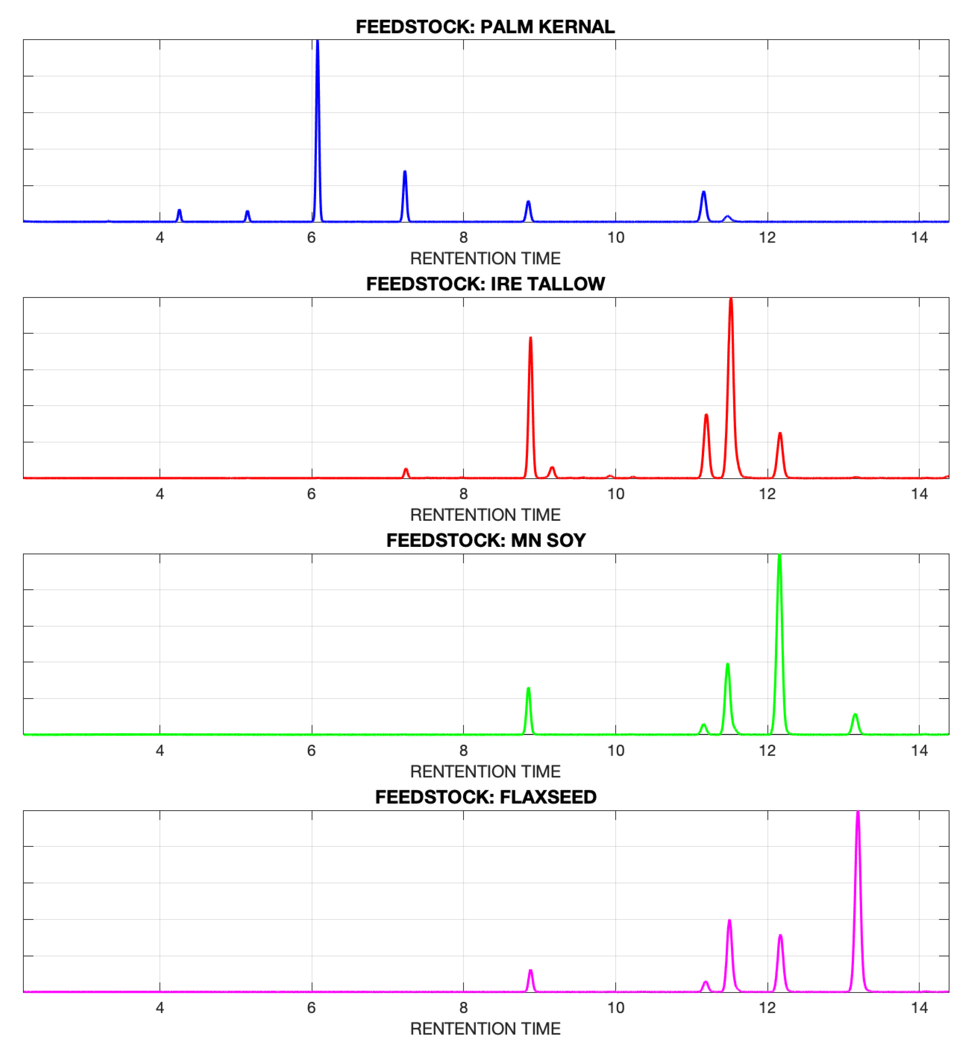
In Figure 2 and Figure 3 we display representative chromatograms acquired on the longer ZB-FFAP column (Figure 2) and shorter DB-FFAP column (Figure 3) for the following feedstocks: Palm Kernal, IRE Tallow, MN Soy, and Flaxseed. The DB-FFAP run time was less than half of the ZB-FFAP run time, yet separation of FAMEs on the two columns is comparable. Resolution between peaks was similar for the two columns, with one exception. The C18:1 isomers are slightly resolved (Rs < 1.5) on the longer ZB-FFAP column while they are completely unresolved on the shorter DB-FFAP column. As has been reported previously [9,21], FAME composition changes as a function of oil and fat type. Palm biodiesel contained C8-C18 FAMEs with C12 the major contributor to the profile. Tallow contained C14-C18:1 (largest peaks = C16 and C18:1), Soy C16-C18:3 (largest peak = C18:2), and Flaxseed C16-C18:3 (largest peak = C18:3).

4.1. No Alignment within Each Feedstock Type

In an initial exploration of the data, the baseline corrected, unaligned data were first examined to determine any statistical differences between columns ZB-FFAP and DB-FFAP. For each feedstock type, the data, comprised of 6 sample runs per column, were PC transformed and the cumulative percent variance was computed. For all feedstock types measured on the ZB column, L = 2 PCs were needed to summarize at least 90% of the variability in each data set. However, for the DB column, L = 3 PCs were needed. It should be noted that for a sample of size six, there were only five non-zero PCs and so the maximum L can be is five.
The MD, F-statistic, and corresponding p-value for each feedstock type were then computed using L = 3 PCs. The values of the MD ranged from 6.03 × 10 30 to 1.48 × 10 31 and all corresponding p-values were 1. This analysis was repeated using L = 5 PCs and found the MD ranged from 9.47 × 10 29 to 2.62 × 10 31 , and again all corresponding p-values were 1. These small MD values indicate reproducibility within the feedstock groups as well as significant similarity across the data sets (column dimension). Thus, when evaluating the data within a specific feedstock type, the unaligned data produced by each column were not statistically significantly different. Furthermore, it should be noted that the results were invariant to the criterion used to select L.

4.2. Alignment within Each Feedstock Type

Next, an investigation of the effect of COW alignment on the MD and our evaluation of statistical differences between the columns was conducted. COW parameters (segment length, maximum warp) were determined that would optimally align the data so that the MD was minimum and corresponding p-value was as close to 1 as possible. Since the alignment and PC transformation were conducted only within a fixed feedstock type, a target chromatogram within the 6 runs that had the maximum SI was chosen. The data were then aligned using all possible combinations of segment length and maximum warp (as outlined in the Methods section) for each column condition:
ZB i = ( seg . length , max . warp ) i = 1 , 2 , , I DB j = ( seg . length , max . warp ) j = 1 , 2 , , J ,
where I and J denote the total number of possible (segment length, maximum warp) combinations for the ZB-FFAP and DB-FFAP columns, respectively.
For each feedstock type and combination of COW parameters, the aligned data comprised of 6 sample runs per column were PC transformed. A MD based on L = 5 PCs was then computed as a function of data from each column aligned with a given set of parameters ZB i and DB j
M D i j = f ( data ZB i , data DB j ) ,
and the result stored in an I × J matrix. A corresponding matrix of p-values was derived using Equation (5).
The MD, corresponding p-value, and optimal parameters ZB i and DB j that minimize the MD using L = 5 PCs are listed in Table 1. The values of the MD were effectively zero, which produced p-values of 1, again indicating reproducibility in replica runs and similarity across the data sets. It should be noted that the minimum MD did not occur using the same set of parameters for each feedstock type. However, this was expected as the feedstocks have peaks of different widths and magnitudes, which occur in different locations along the time axis. It would be unusual for one set of parameters to optimally align such different types of data. Thus, when evaluating the aligned data within a specific feedstock type, the PC scores derived from the aligned data produced by each column were not statistically different. Lastly we note that the values of MD and corresponding p-value computed using L = 3 PCs were equivalent to those in Table 1, and thus not included.

4.3. Alignment across Feedstock Types

Finally, an investigation of the effect of COW alignment across all feedstock types on the MD and our evaluation of statistical differences between the columns was conducted. In this study, data from all of the feedstocks (six runs per feedstock, 12 feedstock types) were combined into a single data set for each column condition. COW parameters were determined to optimally align the data and result in a minimum MD. Since the alignment and PC transformation were conducted across feedstock types, a target chromatogram was chosen across all 72 chromatograms that had maximum SI (see Figure 1). As in the previous analysis, data were aligned using all possible combinations of segment length and maximum warp for each column condition. This global alignment method is typical for PCA of chromatographic data.
In Table 2 and Table 3, the MD, p-value, and COW alignment parameters (segment length and maximum warp) are presented for each feedstock. The MD was computed using both L = 3 PCs (Table 2) and L = 5 PCs (Table 3), in order to be able to compare results across analysis condition. These were chosen based on our findings in Section 4.1: no alignment within each feedstock type, where it was observed that the number of PCs needed to summarize 90% of the variability in both unaligned data sets was L = 3 and the number of non-zero PCs within each feedstock type was L = 5 .
As shown in Table 2 and Table 3, the MD values are all small and the p-values for each feedstock type are close to 1. Again, this confirms reproducibility within the feedstock groups as well as significant similarity across the data sets (column dimension) that have been aligned with a global target. As in the previous subsection, the minimum MD does not occur using the same set of parameters for each feedstock type. Thus, when evaluating the aligned data across feedstock types, the PC scores derived from the aligned data produced by each column were not statistically significantly different.

5. Conclusions

In this work, gas chromatography separation conditions are compared using a statistical metric called the Mahalanobis distance (MD). Chromatograms measured from each column were aligned with the correlated optimized warping algorithm and then principal components analysis (PCA) was applied. PC scores were then used to compute the MD and separation of the data produced by each column was judged by converting the MD to a p-value. The combination of COW parameters that maximized the p-value were unique for each feedstock. All results demonstrate that chromatograms from each column could be optimally aligned to minimize the MD derived from the PC-transformed data. The corresponding p-values for each feedstock type indicated that the two column conditions could produce data that were not statistically significantly different.
This work is the first of its kind to compare data from columns of two different dimensions using chemometric PC analysis. In conclusion, a shorter column with a thinner film provided comparable data relative to a longer column.

Author Contributions

R.R.D. and C.D.B. performed transesterification reactions. R.R.D., C.D.B., A.J.C., and A.M.H. performed experimental investigation (gas chromatography work) and initial analysis of data. A.M.H. wrote the draft of introduction and experimental methods. E.J.S. wrote the draft of methodology and results/discussion. Both authors contributed to supervision of the project (A.M.H. to experiment, E.J.S. to statistics), analysis of results, and review and editing all versions of the paper.

Funding

This research received no external funding.

Acknowledgments

We are greatly appreciative of financial support provided in the form of summer fellowships by Jack D. Rehm, Jr. 1988 and Kathleen Millard Rehm 1989 (R.B.), Katherine L. and Paul S. Stuka 1977 (C.B.), Robert J. Stransky Foundation (A.C.), and the College of the Holy Cross. We also thank TMT Biofuels, ADM Company, Texas Green Manufacturing, Iowa Renewable Energy, and Minnesota Soybean Processors for providing fuel samples.

Conflicts of Interest

The authors declare no conflict of interest.

Abbreviations

The following abbreviations are used in this manuscript:
COWcorrelated optimized warping
FAMEfatty acid methyl esters
GCgas chromatography
MDMahalanobis distance
PCAprincipal components analysis
SIsimilarity index

References

  1. Giddings, J.C. Dynamics of Chromatography Part I Principles and Theory; Marcel Dekker, Inc.: New York, NY, USA, 1965. [Google Scholar]
  2. Knothe, G.; Van Gerpen, J.; Krahl, J. (Eds.) The Biodiesel Handbook; AOCS Press: Urbana, IL, USA, 2005. [Google Scholar]
  3. Cruz-Hernandez, C.; Destaillats, F. Recent advances in fast Gas-Chromatography: Application to the separation of fatty acid methyl esters. J. Liq. Chrom. Rel. Technol. 2009, 32, 1672–1688. [Google Scholar] [CrossRef]
  4. Schale, S.P.; Le, T.M.; Pierce, K.M. Predicting feedstock and percent composition for blends of biodiesel with conventional diesel using chemometrics and gas chromatography-mass spectrometry. Talanta 2012, 94, 320–327. [Google Scholar] [CrossRef] [PubMed]
  5. Hupp, A.M.; Marshall, L.J.; Campbell, D.I.; Waddell Smith, R.; McGuffin, V.L. Chemometric analysis of diesel fuel for forensic and environmental applications. Anal. Chim. Acta 2008, 606, 159–171. [Google Scholar] [CrossRef] [PubMed]
  6. Fortunato de Carvalho Rocha, W.; Schantz, M.M.; Sheen, D.A.; Chu, P.M.; Lippa, K.A. Unsupervised classification of petroleum Certified Reference Materials and other fuels by chemometric analysis of gas chromatography-mass spectrometry data. Fuel 2017, 197, 248–258. [Google Scholar] [CrossRef] [PubMed] [Green Version]
  7. Pauls, R.E. Fast Gas Chromatographic Separation of Biodiesel. J. Chromatogr. Sci. 2011, 49, 370–374. [Google Scholar] [CrossRef]
  8. Turner, T.; Rolland, D.C.; Aldai, N.; Dugan, M.E.R. Rapid Separation of cis9, trans11- and trans7, cis9-18:2 (CLA) isomers from ruminant tissue using a 30 m SLB-IL111 ionic column. Can. J. Anim. Sci. 2011, 91, 711–713. [Google Scholar] [CrossRef]
  9. Goding, J.C.; Ragon, D.Y.; O’Connor, J.B.; Boehm, S.B.; Hupp, A.M. Comparison of GC stationary phases for the separation of fatty acid methyl esters in biodiesel fuels. Anal. Bioanal. Chem. 2013, 405, 6087–6094. [Google Scholar] [CrossRef]
  10. Masood, A.; Stark, K.D.; Salem, N., Jr. A simplified and efficient method for the analysis of fatty acid methyl esters suitable for large clinical studies. J. Lipid. Res. 2005, 46, 2299–2305. [Google Scholar] [CrossRef] [Green Version]
  11. Tauler, R. Multivariate curve resolution applied to second order data. Chemometr. Intell. Lab. 1995, 30, 133–146. [Google Scholar] [CrossRef]
  12. De Luca, S.; Ciotoli, E.; Biancolillo, A.; Bucci, R.; Magri, A.D.; Marini, F. Simultaneous quantification of caffeine and chlorogenic acid in coffee beans and varietal classification of the samples by HPLC-DAD coupled with chemometrics. Environ. Sci. Pollut. R 2018, 25, 28748–28759. [Google Scholar] [CrossRef]
  13. Tauler, R.; Smilde, A.; Kowalski, B. Selectivity, local rank, three-way data analysis and ambiguity in multivariate curve resolution. J. Chemometr. 1995, 9, 31–58. [Google Scholar] [CrossRef]
  14. Maeder, M. Evolving factor analysis for the resolution of overlapping chromatographic peaks. Anal. Chem. 1987, 59, 527–530. [Google Scholar] [CrossRef]
  15. Bahaghighat, H.D.; Freye, C.E.; Gough, D.V.; Synovec, R.E. Comprehensive two-dimensional gas chromatography and time-of-flight mass spectrometry detection with a 50ms modulation period. J. Chromatogr. A 2019, 1583, 117–123. [Google Scholar] [CrossRef] [PubMed]
  16. Azimi, F.; Fatemi, M.H. Multivariate curve resolution-correlation optimized warping applied to the complex GC-MS signals: Toward comparative study of peel chemical variability of Citrus aurantium L. varieties. Microchem. J. 2018, 143, 99–109. [Google Scholar] [CrossRef]
  17. Aliakbarzadeh, G.; Sereshti, H.; Parastar, H. Fatty acids profiling of avocado seed and pulp using gas chromatography-mass spectrometry combined with multivariate chemometric techniques. J. Iran. Chem. Soc. 2016, 13, 1905–1913. [Google Scholar] [CrossRef]
  18. Rocha, W.F.C.; Vaz, B.G.; Sarmanho, G.F.; Leal, L.H.C.; Nogueira, R.; Silva, V.F.; Borges, C.N. Chemometric techniques applied for classification and quantification of binary biodiesel/diesel blends. Anal. Lett. 2012, 45, 2398–2411. [Google Scholar] [CrossRef]
  19. Flood, M.E.; Goding, J.C.; O’Connor, J.B.; Ragon, D.Y.; Hupp, A.M. Analysis of Biodiesel feedstock using GCMS and unsupervised chemometric methods. J. Am. Oil. Chem. Soc. 2014, 91, 1443–1452. [Google Scholar] [CrossRef]
  20. Soares, E.J.; Yalla, G.R.; O’Connor, J.B.; Walsh, K.A.; Hupp, A.M. Hotelling trace criterion as a figure of merit for optimization of chromatogram alignment. J. Chemom. 2014, 29, 200–212. [Google Scholar] [CrossRef]
  21. Flood, M.E.; Connolly, M.P.; Comiskey, M.C.; Hupp, A.M. Evaluation of single and multi-feedstock biodiesel-diesel blends using GC/MS and chemometric methods. Fuel 2016, 186, 58–67. [Google Scholar] [CrossRef]
  22. Jolliffe, I.T. Principal Component Analysis; Springer: New York, NY, USA, 2002. [Google Scholar]
  23. Wold, S.; Esbensen, K.; Geladi, P. Principal Component Analysis. Chemometr. Intell. Lab. 1987, 2, 37–52. [Google Scholar] [CrossRef]
  24. Pearson, K. On lines and planes of closest fit to systems of points in space. Philos. Mag. 1901, 2, 559–572. [Google Scholar] [CrossRef]
  25. Hotelling, H. Analysis of a Complex of Statistical Variable into Principal Components; Warwick and York: Baltimore, MD, USA, 1933. [Google Scholar]
  26. Malmquist, G.; Danielsson, R. Alignment of chromatographic profiles for principal component analysis: A prerequisite for fingerprinting methods. J. Chromatogr. A 1994, 687, 71–88. [Google Scholar] [CrossRef]
  27. Van Nederkassel, A.M.; Daszkowski, M.; Eilers, P.H.C.; Vander Heyden, Y. A comparison of three algorithms for chromatograms alignment. J. Chromatogr. A 2006, 1118, 199–210. [Google Scholar] [CrossRef] [PubMed]
  28. Daszykowski, M.; Walczak, B. Target selection for alignment of chromatographic signals obtained using monochannel detectors. J. Chromatogr. A 2007, 1176, 1–11. [Google Scholar] [CrossRef] [PubMed]
  29. Vest Nielsen, N.; Carstensen, J.M.; Smedsgaard, J. Aligning of single and multiple wavelength chromatographic profiles for chemometric data analysis using correlation optimized warping. J. Chromatogr. A 1998, 805, 17–35. [Google Scholar] [CrossRef]
  30. Tomasi, G.; van den Berg, F.; Andersson, C. Correlation optimized warping and dynamic time warping as preprocessing methods for chromatographic data. J. Chemom. 2004, 18, 231–241. [Google Scholar] [CrossRef]
  31. Andric, F.; Heberger, K. How to compare separation selectivity of high-performance liquid chromatographic columns properly? J. Chromatogr. A 2017, 1488, 45–56. [Google Scholar] [CrossRef] [PubMed] [Green Version]
  32. Nowik, W.; Heron, S.; Bonose, M.; Tchapla, A. Separation system suitability (3S): A new criterion of chromatogram classification in HPLC based on cross-evaluation of separation capacity/peak symmetry and its application to complex mixtures of anthraquinones. Analyst 2013, 138, 5801–5810. [Google Scholar] [CrossRef]
  33. Brereton, R.G.; Lloyd, G.R. Re-evaluating the role of the Mahalanobis distance measure. J. Chemom. 2016, 30, 134–143. [Google Scholar] [CrossRef]
  34. Mahalanobis, P.C. On the generalized distance in statistics. Proc. Natl. Inst. Sci. India Phys. Sci. 1936, 2, 49–55. [Google Scholar]
  35. Mardia, K.V.; Kent, J.T.; Bibby, J.M. Multivariate Analysis; Academic Press: New York, NY, USA, 1979. [Google Scholar]
  36. Skov, T.; van den Berg, F.; Bro, R. Automated alignment of chromatographic data. J. Chemom. 2006, 20, 484–497. [Google Scholar] [CrossRef]
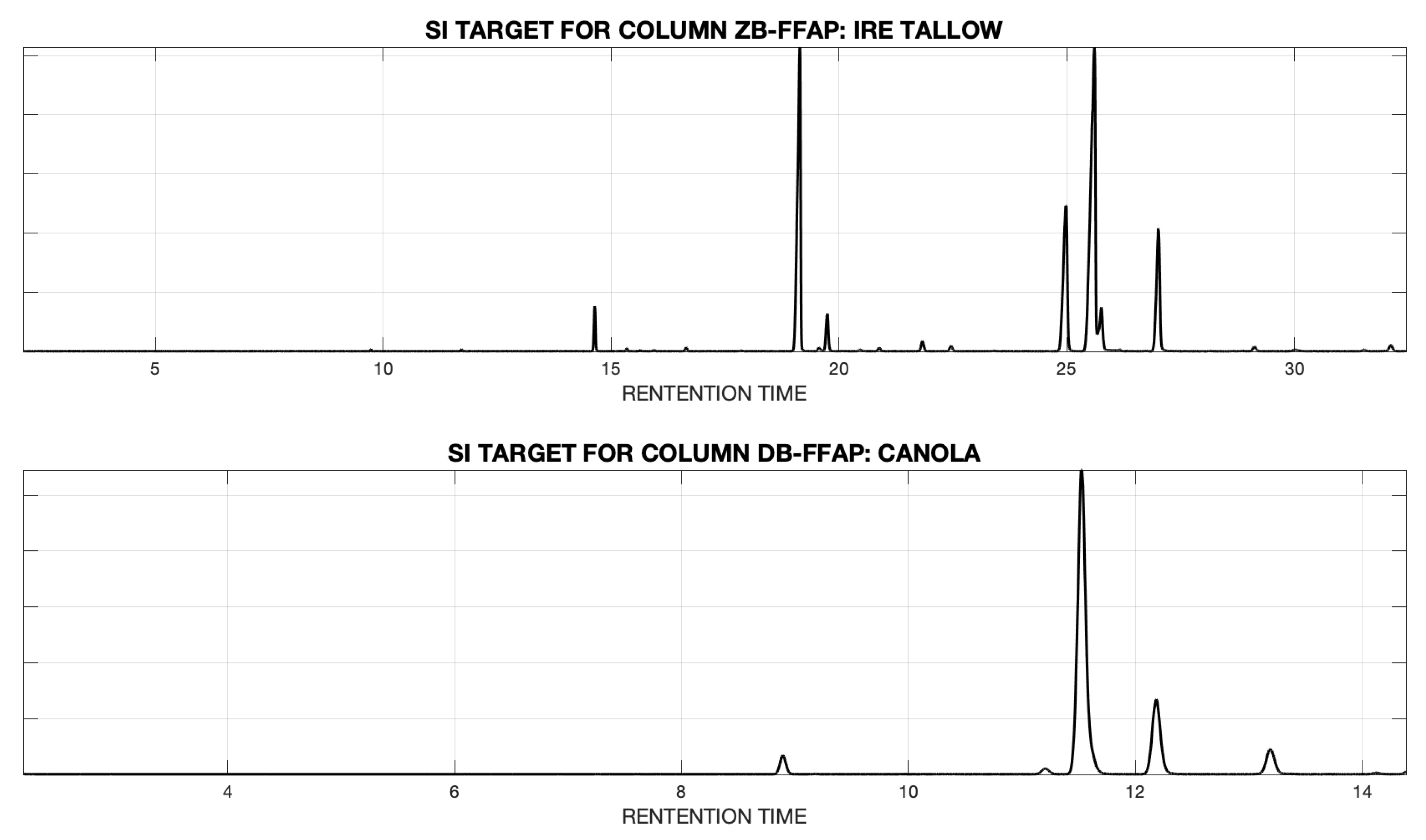
Figure 1. (top) Target chromatogram based on similarity index for column ZB-FFAP data; (bottom) target chromatogram based on similarity index for column DB-FFAP data.
Separations 06 00028 g001
Figure 2. Stacked chromatograms of a B100 biodiesel for various feedstock types using ZB-FFAP (traditional, longer column). Each chromatogram has been normalized to its maximum value for display.
Separations 06 00028 g002
Figure 3. Stacked chromatograms of a B100 biodiesel for various feedstock types using DB-FFAP (shorter, thinner film column). Each chromatogram has been normalized to its maximum value for display.
Separations 06 00028 g003
Table 1. Mahalanobis distance (MD), p-value, and optimal correlated optimized warping (COW) alignment parameters (segment length and maximum warp) for each feedstock, with alignment to a chromatogram from the same feedstock type chosen based on similarity index. The MD was computed based on L = 5 PCs.
FeedstockMDp-ValueSeg. Length (ZB)Max. Warp (ZB)Seg. Length (DB)Max. Warp (DB)
ADM Canola9.83 × 10 33 11914317
Canola1.43 × 10 32 14814218
Coconut8.04 × 10 32 1356247
Flaxseed5.96 × 10 33 1701491
IRE Tallow3.24 × 10 32 1204192
MN Soy2.46 × 10 32 12210138
Palm Kernal2.75 × 10 32 1519171
Safflower6.29 × 10 33 1434216
Soyabean2.15 × 10 32 1149172
Sunflower3.07 × 10 32 1469258
TexasTallow1.85 × 10 32 1154122
Waste Grease1.59 × 10 32 1502278
Table 2. MD, p-value, and optimal COW alignment parameters (segment length and maximum warp) for each feedstock, with alignment to a universal chromatogram chosen based on similarity index. The MD was computed based on L = 3 PCs.
FeedstockMDp-ValueSeg. Length (ZB)Max. Warp (ZB)Seg. Length (DB)Max. Warp (DB)
ADM Canola0.00150.9999677222
Canola0.00041.00006414302
Coconut0.00290.9998439273
Flaxseed0.00101.0000462263
IRE Tallow0.00180.9999692164
MN Soy0.00300.99986813264
Palm Kernal0.01870.9973691581
Safflower0.00300.9998441207
Soyabean0.00180.99994814205
Sunflower0.00180.9999235233
TexasTallow0.00250.9999464152
Waste Grease0.00031.0000562141
Table 3. MD, p-value, and optimal COW alignment parameters (segment length and maximum warp) for each feedstock, with alignment to a universal chromatogram chosen based on similarity index. The MD was computed based on L = 5 PCs.
FeedstockMDp-ValueSeg. Length (ZB)Max. Warp (ZB)Seg. Length (DB)Max. Warp (DB)
ADM Canola0.32940.98336411167
Canola0.11190.99866013184
Coconut0.10470.9988526102
Flaxseed0.40010.9747583208
IRE Tallow0.13560.9978686161
MN Soy0.62570.9384505152
Palm Kernal0.10480.99882215352
Safflower0.22500.9928482251
Soyabean0.11270.9986394212
Sunflower0.08170.9993575132
TexasTallow0.31840.9845381182
Waste Grease0.09320.9991351142