Toward Mechanism-Driven Control: A Soft-Sensor for Zeta Potential and Settling-Decisive Parameters in Coal Slime Water Treatment

Abstract

Intelligent dosing in coal slime water treatment remains a challenge due to the lack of real-time and solid hardware-based measurement of key microscopic parameters governing the settling process, particularly zeta potential. This study proposes a soft-sensor method using Sparrow Search Algorithm-optimized Extreme Learning Machine (SSA-ELM) to simultaneously predict four critical settling process parameters: settling velocity, supernatant turbidity, sediment layer height, and zeta potential. Key variables influencing the coal slime water settling process, including coal slime water concentration, fines content, water hardness, pH, and chemical dosage, were investigated, and the experimental data were used as inputs for the development of the prediction model. The prediction performance of the proposed SSA-ELM model was evaluated against standard ELM and SSA-optimized Back Propagation (BP) models. The results demonstrate that the SSA-ELM model achieved superior prediction accuracy for all parameters, with R² values ranging from 0.95 to 0.98, while maintaining favorable computational efficiency. This study establishes a method for virtual measurement of zeta potential, providing a crucial data foundation for developing mechanism-driven, intelligent dosing systems aimed at precise intelligent control and reduced chemical consumption for coal preparation plants.

1. Introduction

Coal is a critical source of power on our planet, particularly in countries such as China, accounting for 33% of electricity generation today. The world’s appetite for energy is still far from being met [1,2,3]. Under the pressure of the global clean energy transition, the continued reliance on coal necessitates its cleaner and more efficient utilization to balance energy security, economic growth, and carbon reduction. Coal preparation enables high-efficiency, low-emission combustion, facilitating graded utilization to maximize value and minimize environmental impact [4,5]. In China, the mature and widely implemented wet coal preparation process, although efficient, comes at the cost of generating large volumes of high-concentration slime water [6]. Efficient coal slime water treatment is essential because it ensures coal recovery and economic benefits, conserves fresh water resources while preventing polluted water discharge, and safeguards stable raw coal throughput via reliable system operation [7]. Yet, with deeper mining and increased mechanization, raw coal now contains more fines and clay minerals, such as montmorillonite and kaolinite, which readily slake and disperse in water to form stable colloids in the slurry treatment system [8]. These ultra-fine particles typically carry a negative surface charge and resist natural settling due to electrostatic repulsion and Brownian motion, severely impairing the closed-loop washing system and stable operation [9,10,11]. To address this challenge, flocculants and coagulants are therefore routinely added to destabilize this colloidal slurry system and accelerate settling [12].

Dosage control in most Chinese coal preparation plants still relies on manual, experience-based operation and delayed indicators such as supernatant turbidity [13,14]. This approach fails to respond to real-time changes in slime water concentration, flow rate, or particle size distribution [15], often leading to chemical overdosing or underdosing, which causes high turbidity, “black water”, unstable sediment layer height, rake jamming, and ultimately compromises plant safety and profitability [13,16,17]. Real-time, closed-loop intelligent dosing systems offer a critical solution that enhances automation level and enables sustainable, intelligent operation in the coal industry, with recent applications demonstrating substantial economic benefits. For instance, in Buliangou Coal Preparation Plant, an intelligent dosing system reduced coagulant consumption by 58.76% and flocculant consumption by 45.75%, achieving an annual cost saving of 165,400 CNY while lowering labor intensity and labor costs [13]. In Wangpo Coal Preparation Plant, the intelligent dosing system reduced flocculant usage by 8.56% and filter aid usage by 10.25%, achieved unattended operation, and significantly improved thickening and filtration efficiency, resulting in total annual savings of approximately 870,000 CNY in labor, electricity, and material costs, while also reducing operational accidents [15]. Similarly, Menkeqing Coal Preparation Plant reported a flocculant consumption reduction of 24.9% after three months of operation [18,19]. These examples indicate that intelligent dosing can significantly reduce chemical consumption, typically ranging from 8% to 60% depending on plant-specific conditions such as feed composition, scale, and operating parameters.

Intelligent dosing systems integrate advanced sensing, process modeling, and smart control algorithms to dynamically optimize chemical dosage [20]. Extensively studied and applied in municipal wastewater treatment, these systems typically adopt a “feedforward+feedback+intelligent decision-making” architecture [21]. The model-based feedforward channel usually uses measurable parameters like turbidity, pH, and flow rate with mathematical models such as neural networks for preliminary prediction, and the feedback loop often takes indicators like effluent turbidity and algorithms such as Proportional-Integral-Derivative (PID), fuzzy control, or model predictive control (MPC) for fine-tuning [22,23,24,25,26]. However, coal slime water treatment is more challenging because its chemical dosing is highly sensitive to mineral composition, water chemistry and particle size distribution, making sole reliance on turbidity feedback inadequate for managing its nonlinear dynamics [17].

Most intelligent coal slime water dosing systems use basic feedback control driven by macroscopic indicators like feed concentration, overflow turbidity, and mud line height [13,15,18,19,27,28]. Although the reported 8–60% chemical dosage reduction demonstrates the effectiveness of current intelligent dosing systems, actual performance varies considerably across plants. This variation stems from overlooked operational conditions—such as coal slime concentration, fines content, water hardness, and coagulant-to-flocculant ratio. More fundamentally, those macroscopic indicators reflect settling outcomes rather than underlying causes. The resulting models lack insight into key microscopic mechanisms, leading to poor generalization and weak adaptability to changing conditions, with a “black-box” nature and being far from mechanism-based control. Achieving a leap from empirical to precise dosing requires real-time monitoring of key microscopic parameters that govern colloidal stability, such as zeta potential [29,30]. Zeta potential quantifies the net surface charge of a particle within its electrical double layer and directly determines electrostatic repulsion between particles [31]. Coagulants and flocculants primarily function by reducing their absolute value via charge neutralization, double-layer compression, or bridging [32,33]. Utilizing zeta potential as a core feedback or control target offers a pathway toward truly mechanism-based, robust, and cost-effective dosing. However, on-site conditions (high solids concentration, abrasiveness, variable mineral composition, etc.) make reliable zeta potential online monitoring impossible due to sensor clogging, wear, and interference. This lack of a dependable feedback signal poses a fundamental barrier to mechanism-driven intelligent coal slime water treatment.

Confronting the challenge of direct hardware measurement for critical coal slime water settling parameters, soft-sensor method powered by machine learning offers a promising solution, as exemplified by a recent study that developed a multiple linear regression (MLR) soft sensor for real-time process control in a full-scale wastewater treatment plant [34]. For soft sensing of key parameters in coal slime water treatment, Shao et al. [35] developed a Particle Swarm Optimization-Least Squares Support Vector Machine (PSO-LSSVM) model to predict thickener supernatant turbidity, achieving 92.38% accuracy. Wu et al. [28] proposed a Gravitational Search Algorithm (GSA) optimized LSSVM model for sediment layer thickness prediction, with a relative error within 9%. For chemical dosage prediction, Extreme Learning Machine (ELM) offers fast training speed and strong generalization [21]. Wang et al. reported relative errors of 7.41% (ELM) and 10.79% (Back Propagation, BP) for frother dosage prediction in coal slime flotation [36] However, traditional ELM suffers from unstable predictions due to random weight initialization [28]. The Sparrow Search Algorithm (SSA), a swarm intelligence optimization algorithm, has been proven to further boost ELM performance due to its fast convergence and outstanding optimization capability [37,38] Still, most existing work focuses on predicting macroscopic indicators, while an integrated soft sensor targeting key settling parameters (settling velocity, zeta potential, etc.) is lacking, particularly the use of zeta potential for mechanism-based dosing [14,39].

Even as of 2025, China’s coal preparation intelligent construction remains at an early stage, hindered by insufficient technological depth, core instrumentation bottlenecks, and the transition from experience-based to data-driven and, ultimately, mechanism-driven control [40]. To address these challenges, this study proposes an SSA-ELM-based soft-sensor approach for simultaneously “measuring” four important settling parameters: settling velocity, supernatant turbidity, sediment layer height, and—crucially—zeta potential. The novel inclusion of zeta potential is particularly significant. It serves as a key microscopic parameter governing colloidal stability and flocculation efficiency, yet remains inaccessible to direct hardware measurement under on-site conditions. This constitutes a core instrumentation bottleneck that limits the advancement of intelligent dosing in coal slime water treatment systems. By enabling virtual measurement of zeta potential alongside conventional settling outcomes, this work aims to provide the essential data foundation for transitioning from outcome-based data-driven control toward “data- and mechanism-dual-driven” control, thereby supporting the intelligent transformation of coal preparation plants toward more precise, adaptive, and sustainable operation.

2. Materials and Methods

2.1. Preparation of Coal Slime Water Samples

The raw coal sample used in this study was obtained from the Shangwan Coal Preparation Plant, Shendong Coal Preparation Center, China Energy Investment Group. The sample was sequentially crushed using a jaw crusher (model EP-3, Hebi Metallurgical Machinery Equipment Co., Ltd. Tangshan, China) and a roller crusher (model B, Hebi Tianguan Instrument & Meter Co., Ltd., Shijiazhuang, China) to a nominal top size of 0.5 mm, followed by thorough mixing. The ash content of this prepared raw coal was measured to be 10%. A simulated coal slime sample (designated as CS-19) with an elevated ash content of 19% was prepared by blending the raw coal with gangue at a mass ratio of 11:2.

To investigate the influence of fine particle content on the settling process of coal slime water, CS-19 was ground for varying durations using a standard sample preparation grinder (model KEP-FK200A, Zhenjiang Kerui Sample Preparation Equipment Co., Ltd., Zhenjiang, China), producing a series of samples with progressively higher content of fine particles. Each ground sample was thoroughly homogenized, and its particle size distribution was determined via sieve analysis conducted in accordance with the Chinese standard MT/T58-93 (Test Method for Sieve Analysis of Coal Powder) [41]. The proportion of particles finer than 0.045 mm, a key indicator of fineness, was quantified for each grinding interval. The relationship between grinding duration and the content of this fine fraction is summarized in

Table 1. Percentage of particles finer than 0.045 mm in coal slime as a function of grinding time.

Grinding Time (s)	0	2	10	20	65	90	120
Percentage (<0.045 mm) (%)	24	33	39	49	57	69	81

.

2.2. Experimental Data Collection of Coal Slime Water Settling Process

To construct a prediction model for coal slime water settling parameters, this study conducted the following settling experiments and key parameter measurements, collecting 100 sets of experimental data for model training and testing.

2.2.1. Settling Test

Settling tests were conducted following the Chinese standard MT 190-1988 (Test Method for Settling of Coal Slurry Water in Coal Preparation Plants) [42]. The procedure was as follows: a 30 g/L coal slime suspension was first stirred at 500 rad/min for 5 min using a magnetic stirrer (model LC-DMS-S, Shanghai Licheng Bangxi Instrument Technology Co., Ltd., Shanghai, China). The suspension was then transferred to a 500 mL graduated settling cylinder and inverted five times to ensure homogeneity. Subsequently, a specified dosage of a 5000 ppm polyaluminum chloride (PAC, Analytical Grade, Tianjin Damao Chemical Reagent Factory, Tianjin, China) stock solution was added, and the cylinder was inverted another five times. This was immediately followed by the addition of a specified dosage of a 1000 ppm polyacrylamide (PAM, Analytical Grade, molecular weight ~12 million, Shanghai Macklin Biochemical Technology Co., Ltd., Shanghai, China) solution, with the cylinder inverted five times again. Timed settling was then initiated.

The position of the mud line (the interface between the clarified supernatant and the settling solids) was recorded as a function of time. In accordance with the Chinese standard MT 190-1988, the initial settling velocity (ISR) was determined from the data collected within the first 60 s. The height of the mud line (H_i) was observed and recorded at specific time intervals (e.g., 0, 5, 10, 15, 20, 25, 30, … s). The ISR (V, in cm/min) was then calculated from the linear segment of the initial settling curve using the following formula:

$$\mathrm{V}={\displaystyle \frac{\mathrm{M}\sum _{\mathrm{i}=\mathrm{A}}^{\mathrm{B}}{\mathrm{T}}_{\mathrm{i}}{\mathrm{H}}_{\mathrm{i}}-\left(\sum _{\mathrm{i}=\mathrm{A}}^{\mathrm{B}}{\mathrm{T}}_{\mathrm{i}}\right)\left(\sum _{\mathrm{i}=\mathrm{A}}^{\mathrm{B}}{\mathrm{H}}_{\mathrm{i}}\right)}{\mathrm{M}\sum _{\mathrm{i}=\mathrm{A}}^{\mathrm{B}}{{\mathrm{T}}_{\mathrm{i}}}^2-{\left(\sum _{\mathrm{i}=\mathrm{A}}^{\mathrm{B}}{\mathrm{T}}_{\mathrm{i}}\right)}^2}}\times 6$$

(1)

where V is the initial settling velocity of the clarification interface (cm/min); T_i is the cumulative time at a specific observation point i (i = 0, 1, 2, 3, … n), in seconds; H_i is the corresponding cumulative descent distance of the clarification interface at T_i, in millimeters; and A and B are the sequence numbers marking the start and end points, respectively, of the linear segment on the settling curve. The summation is performed over M data points within this linear segment from A to B.

After 10 min of settling, the final sediment thickness was recorded. A 30 mL sample of the supernatant was carefully extracted using a pipette from a position 10 cm below the water surface for subsequent analysis of turbidity and zeta potential.

2.2.2. Zeta Potential Measurement

The colloidal stability of the system was assessed by measuring the zeta potential ($\zeta$) of the supernatant to indicate whether coagulant addition is insufficient or excessive, thus offering a rational basis for dosing control. Directly after the 10 min settling test, a sample was collected and analyzed using a Malvern ZEN3690 Zetasizer Nano instrument (Malvern Panalytical, Malvern, UK). All measurements were performed at 25 °C and repeated three times to ensure reproducibility.

2.2.3. Turbidity Measurement

The clarity of the supernatant was quantified by measuring its turbidity. A WZS-188 turbidimeter (Shanghai Yidian Scientific Instruments Co., Ltd., Shanghai, China) was used after a 30 min warm-up and calibration with ultrapure water. The collected supernatant sample was shaken gently to homogenize it, poured into the instrument’s sample cell, and the turbidity value was read and recorded after approximately 10 s.

2.3. Construction of the SSA-ELM Prediction Model

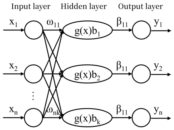
ELM, a type of feedforward neural network, was selected as the core algorithm for modeling the coal slime water sedimentation process; see Figure 1 for its topology diagram [25]. This selection is based on ELM’s suitability for scenarios with limited data, as well as its widespread adoption in industrial soft sensor applications for nonlinear process modeling, where labeled samples are typically scarce [43,44,45,46]. Its key characteristic is that the weights between the input and hidden layers and the hidden layer thresholds are randomly assigned without iterative tuning, while the output layer weights are derived analytically from these random parameters. This gives ELM distinct advantages over traditional neural networks, including an extremely fast learning speed, strong generalization capability, superior function approximation ability, noise resistance, and minimal need for manual intervention—properties that are highly desirable for real-time industrial prediction tasks [47,48]. Accordingly, the ELM model in this study adopts the classical single-hidden-layer architecture—which preserves its inherent advantages of fast training and low computational complexity while also helping mitigate the risk of overfitting given the limited dataset—and is formulated as follows [49,50].

For an ELM with k hidden layer nodes, its output is given by:

$$y_n\left(x\right)={\sum }_{i=1}^k{\beta }_i{g}_i\left(x\right)={\sum }_{i=1}^L{\beta }_{i}g\left(w_i\ast x_j+b_i\right),j=1,\dots ,N$$

(2)

where n is the number of training samples; $w_i$ represents the connection weight between the input layer and the hidden layer; ${\beta }_i$ denotes the connection weight between the hidden layer and the output layer; $g_i\left(x\right)$ is the activation function; $b_i$ is the threshold of the i-th hidden layer node; x and y are the input vector and output vector of the model, respectively.

Expressing ELM in matrix form yields:

$$H\beta =T$$

(3)

where H is the hidden layer output matrix, β is the output layer weight matrix, and T is the target matrix of the model. By solving the least squares solution of this linear model, the formula for calculating the output layer weights is obtained:

$$\beta =H^{+}T$$

(4)

where $H^{+}$ is the Moore–Penrose generalized inverse of the hidden layer output matrix H. This solution approach is crucial for ELM to maintain a good generalization performance.

However, under complex and non-linear industrial conditions, the random initialization of ELM’s input weights and hidden biases can lead the model to converge to local optima, thereby compromising prediction accuracy and stability. To improve the robustness and prediction performance of ELM, the SSA was employed to globally optimize these internal parameters of ELM. SSA is noted for its efficient global search capability, rapid convergence, and effective escape from local optima [38,51], making it well-suited to address the insufficient prediction accuracy that may arise from ELM’s randomly generated parameters in modeling complex processes such as coal slime water settling.

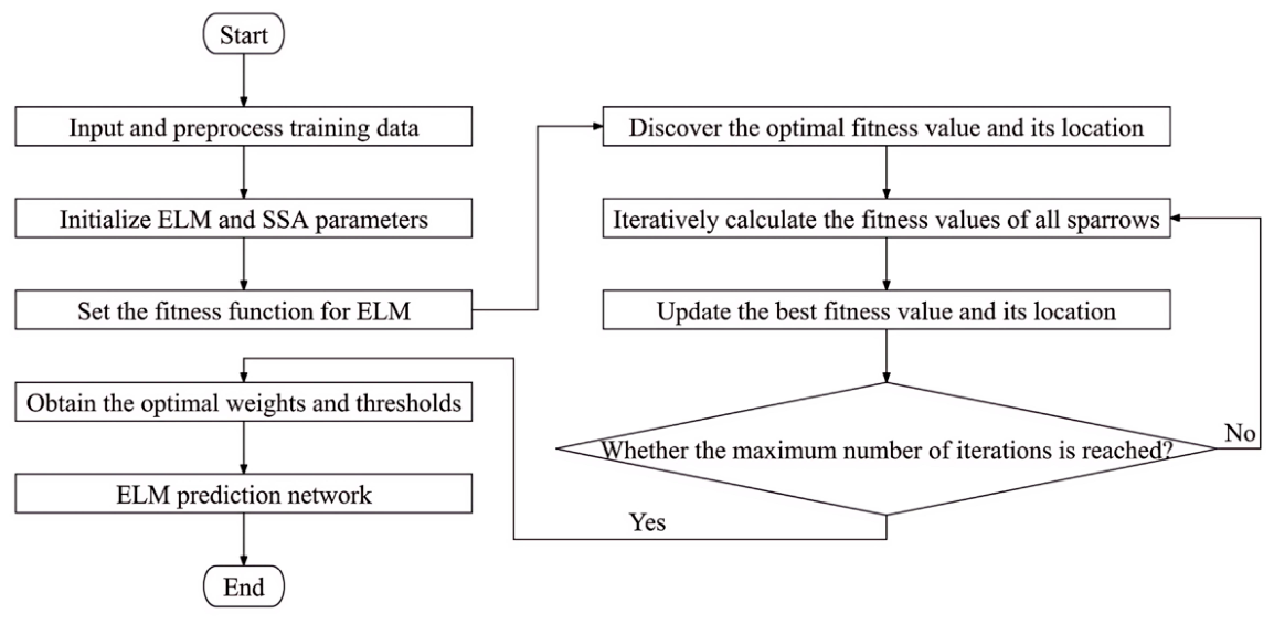
The SSA-ELM model for predicting coal slime water settling parameters in this study was developed in MATLAB (All data analyses were performed using MATLAB (Version R2025a, The MathWorks Inc., Natick, MA, USA).) following the structured framework illustrated in Figure 2. The key steps are outlined below.

(1)

Data Normalization: All input variables were normalized to the range [0, 1] using the min-max normalization method to eliminate dimensional discrepancies among the variables and improve the convergence speed and fitting accuracy.

(2)

Model Parameter Initialization: With reference to the Kolmogorov theorem, the number of hidden layer nodes in the ELM was set within the range of 1–50. After comparing model performance metrics across multiple experimental groups, the optimal number of nodes was determined to be 30. Meanwhile, the parameters of the SSA were initialized with a population size of 30, a maximum iteration number of 60, a warning threshold of 0.6, a discoverer proportion of 0.7, and a scout proportion of 0.2.

(3)

SSA-based Global Parameter Optimization: Following the population position update rules of SSA [38], the positions of discoverers, followers, and scouts were iteratively updated to search for the optimal input-to-hidden layer weights and hidden layer thresholds of the ELM.

(4)

ELM Model Training and Prediction: The Sigmoid function was selected as the activation function of the ELM (determined by comparing the modeling performance of three classic activation functions: Sigmoid, Sine, and Hardlim). The parameters optimized by SSA were then substituted into the ELM to complete model training, and regression predictions were performed on the testing data set.

(5)

Model Performance Evaluation: The mean absolute error (MAE), mean absolute percentage error (MAPE), mean squared error (MSE), root mean squared error (RMSE), and coefficient of determination (R²) were selected as evaluation metrics. The core formulas are given below [52,53,54]:

$$\mathrm{M}\mathrm{A}\mathrm{P}\mathrm{E}={\displaystyle \frac{1}{m}}{\sum }_{i=1}^m\left|{\displaystyle \frac{y_i-f\left(x_i\right)}{y_i}}\right|\times 100\%$$

(5)

$$\mathrm{M}\mathrm{S}\mathrm{E}={\displaystyle \frac{1}{m}}{\sum }_{i=1}^m{\left(y_i-f\left(x_i\right)\right)}^2$$

(6)

$$\mathrm{M}\mathrm{A}\mathrm{E}={\displaystyle \frac{1}{m}}{\sum }_{i=1}^m\left|y_i-f\left(x_i\right)\right|$$

(7)

$$\mathrm{R}\mathrm{M}\mathrm{S}\mathrm{E}=\sqrt{{\displaystyle \frac{1}{m}}{\sum }_{i=1}^m{\left(y_i-f\left(x_i\right)\right)}^2}$$

(8)

$${\mathrm{R}}^2=1-{\displaystyle \frac{{\sum }_{i=1}^m{\left(y_i-f\left(x_i\right)\right)}^2}{{\sum }_{i=1}^m{\left(y_i-\overline{y}\right)}^2}}$$

(9)

where m is the number of test samples, y_i is the actual value (experimental value in this study) of the parameter, f(x_i) is the predicted value from the model, and y is the average of the actual values. Because MAPE can be unreliable for very small actual values, R² and RMSE are used as the primary evaluation metrics, with MAPE reported for reference only.

2.4. Model Performance Test

A prediction model for coal slime water settling parameters based on SSA-ELM was established using the 100 sets of experimental data collected from settling tests. To evaluate model performance and stability, we adopted a Monte Carlo cross-validation approach—also known as repeated random sub-sampling—which is particularly suitable for small datasets [55,56]. Specifically, we performed five independent runs with random data splits (70% for training, 30% for testing). To evaluate the performance of the proposed SSA-ELM model in this research, comparisons were made with the traditional ELM model and the reported high-performance SSA-BP model. The SSA-BP model has been successfully applied in water treatment-related predictions, such as effluent quality forecasting and membrane fouling prediction, and is therefore selected as a robust benchmark to evaluate the advancement of the proposed SSA-ELM model [57,58]. To ensure a fair comparison, both SSA-ELM and SSA-BP were configured with identical SSA parameters (population size 30, maximum iterations 60, as described in Section 2.3), and both models adopted the same single-hidden-layer architecture with 30 hidden nodes. For the BP network, the learning rate was set to 0.01, the maximum number of epochs was set to 500, and the activation function was set to Sigmoid, selected based on preliminary trials to ensure convergence. All models were executed on the same hardware platform using MATLAB to eliminate hardware-related variability. All three models take six variables—slime water concentration, flocculant dosage, coagulant dosage, pH, water hardness, and fine particle content—as input to predict four key settling parameters: settling velocity, supernatant turbidity, sediment layer height, and $\zeta$ potential. Since the results vary slightly with each model run, the average outcomes from the five independent runs were used for comparison to minimize random variations, and the standard deviations are reported to indicate prediction stability.

3. Results and Discussion

3.1. Characterization of Coal Slime Sample

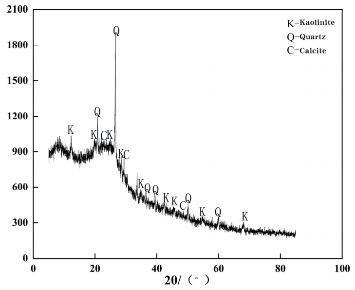
The mineral composition significantly influences the difficulty of coal slime settling. Therefore, X-ray diffraction (XRD, D8 ADVANCE, Bruker Karlsruhe, Germany) was performed on the coal slime sample, and the pattern (as shown in Figure 3) identified quartz, kaolinite, and calcite as the main mineral constituents. These minerals are all hydrophilic, and a higher content of them is generally unfavorable for coal slime water treatment. This hydrophilicity, combined with their pH-dependent surface charge, critically influences dewatering.

According to the Derjaguin–Landau–Verwey–Overbeek (DLVO) theory, the net interaction energy between particles is governed by the balance between van der Waals attraction and electrostatic repulsion, with the latter being directly determined by the surface potential, which is experimentally characterized by the zeta potential of the coal slime particles [31]. The point of zero charge (PZC) for quartz is approximately 2, so its surface is positively charged at pH < 2 and negatively charged at pH > 2 [59]. As a typical phyllosilicate clay mineral, kaolinite has a layered structure and anisotropic charging properties, with PZC < 3 for its Si-basal plane (similar to SiO₂), 6~8 for Al-basal plane, and around 5 for edge surfaces [60]. Changes in pH significantly affect the charge on the Al-basal plane and edge surfaces. Calcite has a higher PZC (~8.9) [61]. This leads to two challenges. Firstly, under high-pH conditions, all particle surfaces are strongly negatively charged. The dominant electrostatic repulsion over the van der Waals attraction causes high dispersion. Under low-pH conditions, while electrostatic repulsion is reduced, the heterogeneous surface charges can drive the formation of complex, voluminous aggregates (such as card-house structures), which trap water and similarly impede efficient dewatering [60].

Therefore, this study investigates key influencing factors: coal slime water concentration, fine particle content (reflecting hard-to-settle degree), water hardness, and pH (which jointly determine surface charge and thus coagulant and flocculant demand). These factors are used as input variables to predict key settling parameters: settling velocity, supernatant turbidity, sediment layer height, and ζ potential. This enables optimal chemical dosages determination for precise settling control under diverse operating conditions.

3.2. Impact Factors of Coal Slime Water Settling Process

In coal preparation plants, the concentration of coal slime water, the content of difficult-to-settle fine particles, and water quality (e.g., pH, hardness) often fluctuate. These factors notably impact the settling and thickening process of coal slime water in the thickener. To establish the relationship between chemical additive dosages, settling performance and its influencing factors, 100 sets of coal slime water settling test data were collected for model construction. These experiments examined the effects of the four factors on settling velocity, supernatant turbidity, sediment layer height, and ζ potential under varying chemical dosages. A subset of the results is presented in

Table 2. Experimental data ¹ of coal slime water settling process.

No.	CCLW g/L	DC kg/t	DF kg/t	pH	WH mg/L	dFC %	V cm/min	T NTU	HSL cm	${\mathbf{\psi }}_{\mathsf{\xi }}$ mV
1	10.00	0.75	0.25	9.00	0.00	49.00	85.84	38.30	0.60	−12.98
2	15.00	0.75	0.25	9.00	0.00	49.00	79.01	26.10	1.10	−14.50
3	20.00	0.75	0.25	9.00	0.00	49.00	72.17	13.89	1.60	−16.01
4	25.00	0.75	0.25	9.00	0.00	49.00	70.11	10.35	2.10	−16.88
5	30.00	0.75	0.25	9.00	0.00	49.00	68.04	6.80	2.60	−17.76
6	32.50	0.75	0.25	9.00	0.00	49.00	64.62	6.97	2.68	−18.36
7	35.00	0.75	0.25	9.00	0.00	49.00	61.21	7.13	2.75	−18.97
8	37.50	0.75	0.25	9.00	0.00	49.00	57.79	7.29	2.83	−19.58
9	40.00	0.75	0.25	9.00	0.00	49.00	54.37	7.45	2.90	−20.18
10	42.50	0.75	0.25	9.00	0.00	49.00	51.79	6.80	2.95	−19.78
11	45.00	0.75	0.25	9.00	0.00	49.00	49.22	6.14	3.00	−19.38
12	47.50	0.75	0.25	9.00	0.00	49.00	46.64	5.49	3.05	−18.98
13	50.00	0.75	0.25	9.00	0.00	49.00	44.06	4.83	3.10	−18.58
14	30.00	0.70	0.25	3.00	0.00	49.00	48.59	8.24	2.71	−0.74
15	30.00	0.70	0.25	4.00	0.00	49.00	49.85	7.24	2.71	−4.20
16	30.00	0.70	0.25	5.00	0.00	49.00	51.10	6.25	2.71	−7.66
17	30.00	0.70	0.25	6.00	0.00	49.00	51.92	8.40	2.71	−11.44
18	30.00	0.70	0.25	7.00	0.00	49.00	52.73	10.55	2.71	−15.21
19	30.00	0.70	0.25	8.00	0.00	49.00	59.64	8.76	2.60	−16.89
20	30.00	0.70	0.25	9.00	0.00	49.00	66.54	6.97	2.50	−18.56
21	30.00	0.70	0.25	10.00	0.00	49.00	70.21	7.84	2.50	−23.87
22	30.00	0.70	0.25	11.00	0.00	49.00	73.88	8.71	2.50	−29.18
23	30.00	0.70	0.25	9.00	50.00	49.00	62.97	6.28	2.54	−14.00
24	30.00	0.70	0.25	9.00	100.00	49.00	59.39	5.58	2.59	−9.44
25	30.00	0.70	0.25	9.00	150.00	49.00	57.27	5.00	2.50	−8.99
26	30.00	0.70	0.25	9.00	200.00	49.00	55.15	4.43	2.40	−8.54
27	30.00	0.70	0.25	9.00	250.00	49.00	55.03	4.83	2.35	−8.18
28	30.00	0.70	0.25	9.00	300.00	49.00	54.91	5.23	2.30	−7.83
29	30.00	0.70	0.25	9.00	350.00	49.00	54.24	5.32	2.35	−7.40
30	30.00	0.70	0.25	9.00	400.00	49.00	53.58	5.40	2.40	−6.97
31	30.00	0.70	0.25	9.00	450.00	49.00	55.39	5.30	2.30	−6.54
32	30.00	0.70	0.25	9.00	500.00	49.00	57.21	5.20	2.21	−6.10
33	30.00	0.70	0.25	9.00	0.00	24.00	88.21	8.34	2.30	−16.15
34	30.00	0.70	0.25	9.00	0.00	33.00	78.07	8.24	2.30	−15.85
35	30.00	0.70	0.25	9.00	0.00	39.00	71.92	7.65	2.40	−15.73
36	30.00	0.70	0.25	9.00	0.00	49.00	66.54	6.97	2.50	−18.56
37	30.00	0.70	0.25	9.00	0.00	57.00	57.02	6.38	2.70	−15.81
38	30.00	0.70	0.25	9.00	0.00	69.00	49.52	6.62	2.70	−17.04
39	30.00	0.70	0.25	9.00	0.00	81.00	43.65	8.11	2.80	−17.87
…
96	50.00	1.30	0.15	9.00	200.00	39.00	36.96	2.97	3.50	−8.59
97	50.00	0.50	0.20	11.00	300.00	49.00	41.04	2.98	3.50	−10.19
98	50.00	0.70	0.25	3.00	400.00	57.00	25.29	3.75	3.50	1.93
99	50.00	0.90	0.30	5.00	0.00	69.00	19.12	3.29	4.00	−0.19
100	50.00	1.10	0.35	7.00	100.00	33.00	64.80	7.34	3.70	−8.45

¹ Abbreviations in the table header: C_CSW: coal slime water concentration; D_C: coagulant dosage; D_F: flocculant dosage; WH: water hardness; d_FC: percentage of coal slime particles finer than 0.045 mm; V: settling velocity; T: turbidity; H_SL: sediment layer height; ψ_ξ: zeta potential.

, while the complete set is provided in Appendix A,

Table A1. Complete experimental data of coal slime water settling process.

No.	CCLW g/L	DC kg/t	DF kg/t	pH	WH mg/L	dFC %	V cm/min	T NTU	HSL cm	${\mathbf{\psi }}_{\mathsf{\xi }}$ mV
1	10.00	0.75	0.25	9.00	0.00	49.00	85.84	38.30	0.60	−12.98
2	15.00	0.75	0.25	9.00	0.00	49.00	79.01	26.10	1.10	−14.50
3	20.00	0.75	0.25	9.00	0.00	49.00	72.17	13.89	1.60	−16.01
4	25.00	0.75	0.25	9.00	0.00	49.00	70.11	10.35	2.10	−16.88
5	30.00	0.75	0.25	9.00	0.00	49.00	68.04	6.80	2.60	−17.76
6	32.50	0.75	0.25	9.00	0.00	49.00	64.62	6.97	2.68	−18.36
7	35.00	0.75	0.25	9.00	0.00	49.00	61.21	7.13	2.75	−18.97
8	37.50	0.75	0.25	9.00	0.00	49.00	57.79	7.29	2.83	−19.58
9	40.00	0.75	0.25	9.00	0.00	49.00	54.37	7.45	2.90	−20.18
10	42.50	0.75	0.25	9.00	0.00	49.00	51.79	6.80	2.95	−19.78
11	45.00	0.75	0.25	9.00	0.00	49.00	49.22	6.14	3.00	−19.38
12	47.50	0.75	0.25	9.00	0.00	49.00	46.64	5.49	3.05	−18.98
13	50.00	0.75	0.25	9.00	0.00	49.00	44.06	4.83	3.10	−18.58
14	30.00	0.70	0.25	3.00	0.00	49.00	48.59	8.24	2.71	−0.74
15	30.00	0.70	0.25	4.00	0.00	49.00	49.85	7.24	2.71	−4.20
16	30.00	0.70	0.25	5.00	0.00	49.00	51.10	6.25	2.71	−7.66
17	30.00	0.70	0.25	6.00	0.00	49.00	51.92	8.40	2.71	−11.44
18	30.00	0.70	0.25	7.00	0.00	49.00	52.73	10.55	2.71	−15.21
19	30.00	0.70	0.25	8.00	0.00	49.00	59.64	8.76	2.60	−16.89
20	30.00	0.70	0.25	9.00	0.00	49.00	66.54	6.97	2.50	−18.56
21	30.00	0.70	0.25	10.00	0.00	49.00	70.21	7.84	2.50	−23.87
22	30.00	0.70	0.25	11.00	0.00	49.00	73.88	8.71	2.50	−29.18
23	30.00	0.70	0.25	9.00	50.00	49.00	62.97	6.28	2.54	−14.00
24	30.00	0.70	0.25	9.00	100.00	49.00	59.39	5.58	2.59	−9.44
25	30.00	0.70	0.25	9.00	150.00	49.00	57.27	5.00	2.50	−8.99
26	30.00	0.70	0.25	9.00	200.00	49.00	55.15	4.43	2.40	−8.54
27	30.00	0.70	0.25	9.00	250.00	49.00	55.03	4.83	2.35	−8.18
28	30.00	0.70	0.25	9.00	300.00	49.00	54.91	5.23	2.30	−7.83
29	30.00	0.70	0.25	9.00	350.00	49.00	54.24	5.32	2.35	−7.40
30	30.00	0.70	0.25	9.00	400.00	49.00	53.58	5.40	2.40	−6.97
31	30.00	0.70	0.25	9.00	450.00	49.00	55.39	5.30	2.30	−6.54
32	30.00	0.70	0.25	9.00	500.00	49.00	57.21	5.20	2.21	−6.10
33	30.00	0.70	0.25	9.00	0.00	24.00	88.21	8.34	2.30	−16.15
34	30.00	0.70	0.25	9.00	0.00	33.00	78.07	8.24	2.30	−15.85
35	30.00	0.70	0.25	9.00	0.00	39.00	71.92	7.65	2.40	−15.73
36	30.00	0.70	0.25	9.00	0.00	49.00	66.54	6.97	2.50	−18.56
37	30.00	0.70	0.25	9.00	0.00	57.00	57.02	6.38	2.70	−15.81
38	30.00	0.70	0.25	9.00	0.00	69.00	49.52	6.62	2.70	−17.04
39	30.00	0.70	0.25	9.00	0.00	81.00	43.65	8.11	2.80	−17.87
40	30.00	0.75	0.10	9.00	0.00	49.00	39.26	13.24	2.70	−19.44
41	30.00	0.75	0.13	9.00	0.00	49.00	43.63	10.23	2.60	−19.12
42	30.00	0.75	0.15	9.00	0.00	49.00	48.00	7.22	2.50	−18.79
43	30.00	0.75	0.18	9.00	0.00	49.00	50.16	6.48	2.60	−17.90
44	30.00	0.75	0.20	9.00	0.00	49.00	52.32	5.74	2.70	−17.01
45	30.00	0.75	0.23	9.00	0.00	49.00	60.18	6.27	2.65	−17.38
46	30.00	0.75	0.25	9.00	0.00	49.00	68.04	6.80	2.60	−17.76
47	30.00	0.75	0.28	9.00	0.00	49.00	68.22	7.75	2.60	−17.98
48	30.00	0.75	0.29	9.00	0.00	49.00	68.31	8.22	2.60	−18.09
49	30.00	0.75	0.30	9.00	0.00	49.00	68.40	8.70	2.60	−18.20
50	30.00	0.75	0.33	9.00	0.00	49.00	68.46	16.27	2.65	−18.43
51	30.00	0.75	0.35	9.00	0.00	49.00	68.52	23.85	2.70	−18.67
52	30.00	0.50	0.25	9.00	0.00	49.00	75.64	11.31	2.50	−18.98
53	30.00	0.60	0.25	9.00	0.00	49.00	71.09	9.14	2.50	−18.77
54	30.00	0.70	0.25	9.00	0.00	49.00	66.54	6.97	2.50	−18.56
55	30.00	0.73	0.25	9.00	0.00	49.00	67.29	6.89	2.55	−18.16
56	30.00	0.75	0.25	9.00	0.00	49.00	68.04	6.80	2.60	−17.76
57	30.00	0.80	0.25	9.00	0.00	49.00	68.79	6.71	2.65	−17.35
58	30.00	0.90	0.25	9.00	0.00	49.00	69.54	6.63	2.70	−16.95
59	30.00	1.00	0.25	9.00	0.00	49.00	66.79	6.18	2.70	−16.95
60	30.00	1.10	0.25	9.00	0.00	49.00	64.05	5.73	2.70	−16.95
61	30.00	1.20	0.25	9.00	0.00	49.00	62.68	5.24	2.65	−17.76
62	30.00	1.30	0.25	9.00	0.00	49.00	61.31	4.75	2.60	−18.56
63	30.00	0.70	0.25	9.00	0.00	49.00	66.54	6.97	2.50	−18.56
64	30.00	0.70	0.25	9.00	0.00	28.50	83.14	8.29	2.30	−16.00
65	30.00	0.70	0.25	9.00	0.00	30.75	80.61	8.27	2.30	−15.92
66	30.00	0.70	0.25	9.00	0.00	34.50	76.53	8.10	2.30	−15.82
67	30.00	0.70	0.25	9.00	0.00	36.00	75.00	7.95	2.35	−15.79
68	30.00	0.70	0.25	9.00	0.00	37.50	73.46	7.80	2.38	−15.76
69	30.00	0.70	0.25	9.00	0.00	44.00	69.23	7.31	2.45	−17.14
70	30.00	0.70	0.25	9.00	0.00	46.50	67.89	7.14	2.48	−17.85
71	30.00	0.70	0.25	9.00	0.00	53.00	61.78	6.68	2.60	−17.18
72	30.00	0.70	0.25	9.00	0.00	55.00	59.40	6.53	2.65	−16.50
73	30.00	0.70	0.25	9.00	0.00	63.00	53.27	6.50	2.70	−16.43
74	30.00	0.70	0.25	9.00	0.00	72.00	48.05	6.99	2.70	−17.25
75	30.00	0.70	0.25	9.00	0.00	75.00	46.59	7.37	2.75	−17.46
76	10.00	0.50	0.15	3.00	0.00	33.00	108.60	27.81	0.50	2.45
77	10.00	0.70	0.20	5.00	100.00	39.00	76.80	31.41	1.00	−2.05
78	10.00	0.90	0.25	7.00	200.00	49.00	55.32	21.75	1.00	−7.21
79	10.00	1.10	0.30	9.00	300.00	57.00	59.88	26.64	0.90	−5.61
80	10.00	1.30	0.35	11.00	400.00	69.00	72.00	14.06	1.10	−8.41
81	20.00	0.70	0.15	7.00	300.00	69.00	42.72	10.30	2.10	−8.01
82	20.00	0.90	0.20	9.00	400.00	33.00	71.54	21.20	1.40	−3.10
83	20.00	1.10	0.25	11.00	0.00	39.00	83.52	11.78	1.50	−19.25
84	20.00	1.30	0.30	3.00	100.00	49.00	58.02	8.88	1.80	4.12
85	20.00	0.50	0.35	5.00	200.00	57.00	55.08	8.37	1.70	−3.10
86	30.00	0.90	0.15	11.00	100.00	57.00	47.76	7.45	2.30	−14.33
87	30.00	1.10	0.20	3.00	200.00	69.00	33.00	6.65	2.30	8.37
88	30.00	1.30	0.25	5.00	300.00	33.00	69.36	5.13	2.30	5.02
89	30.00	0.50	0.30	7.00	400.00	39.00	68.04	5.12	2.20	−4.45
90	30.00	0.70	0.35	9.00	0.00	49.00	87.00	11.85	2.70	−13.93
91	40.00	1.10	0.15	5.00	400.00	49.00	34.09	5.75	3.00	13.20
92	40.00	1.30	0.20	7.00	0.00	57.00	35.07	3.22	3.30	−7.25
93	40.00	0.50	0.25	9.00	100.00	69.00	31.47	4.25	3.30	−11.75
94	40.00	0.70	0.30	11.00	200.00	33.00	62.64	3.89	2.80	−8.17
95	40.00	0.90	0.35	3.00	300.00	39.00	50.40	5.35	2.50	3.67
96	50.00	1.30	0.15	9.00	200.00	39.00	36.96	2.97	3.50	−8.59
97	50.00	0.50	0.20	11.00	300.00	49.00	41.04	2.98	3.50	−10.19
98	50.00	0.70	0.25	3.00	400.00	57.00	25.29	3.75	3.50	1.93
99	50.00	0.90	0.30	5.00	0.00	69.00	19.12	3.29	4.00	−0.19
100	50.00	1.10	0.35	7.00	100.00	33.00	64.80	7.34	3.70	−8.45

.

3.2.1. Influence of Coal Slime Water Concentration

To simulate the coal slime water treatment system in good days and bad days, the influence of coal slime water concentration across a range of 10–50 g/L was examined. With coagulant (PAC) and flocculant (PAM) dosages fixed at 0.75 kg/t and 0.25 kg/t respectively, increasing the slurry concentration from 10 to 50 g/L resulted in a decrease in settling velocity from 85.84 to 44.06 cm/min, a general reduction in supernatant turbidity from 38.3 to 4.83 NTU (despite intermediate fluctuations), an increase in sediment layer height from 0.6 to 3.1 cm, and an initial rise followed by a decline in $\zeta$ potential.

The observed decrease in turbidity with increasing slime concentration was primarily due to flocculant overdosing. This was demonstrated in tests with 30 g/L slurry, where increasing the flocculant dosage from 0.1 to 0.35 kg/t caused turbidity to first drop from 13.24 NTU to a minimum of 5.74 NTU at 0.2 kg/t, before rising again to 23.85 NTU at 0.35 kg/t (see Table A1). Notably, $\zeta$ potential exhibited a positive correlation with turbidity throughout this process. Lower $\zeta$ potential corresponded to lower supernatant turbidity, which manifests that strong electrostatic repulsion among negatively charged fine mineral particles is the dominant mechanism hindering effective particle aggregation and fast settling. Hence, obtaining in situ $\zeta$ potential values are essential for determining coagulant and flocculant dosages for the coal slime water treatment process.

3.2.2. Influence of pH

As noted above, pH significantly influences the surface charging properties of clay mineral particles, which are the troublemakers in the coal slime water settling process. To investigate this impact, the pH of coal slime water was adjusted across a range of 3 to 11. As shown in Table 2, increasing pH shifted the $\zeta$ potential from −0.74 mV to −29.18 mV. This shift was accompanied by a faster settling velocity, a thinner sediment layer, and a fluctuation in supernatant turbidity.

Although the increase in pH caused the particles to carry more negative charges (as evidenced by the more negative $\zeta$ potential) the settling performance did not deteriorate. This apparent contradiction suggests that electrostatic repulsion was no longer the rate-limiting factor under these experimental conditions. At pH 3, the system appeared to be in an overdosing state. Although the $\zeta$ potential was −0.74 mV, very close to the isoelectric point, this does not mean all particle surfaces were uncharged [62]. On the contrary, some surfaces of anisotropic coal slime particles (such as kaolinite) likely carried positive charges due to the overdosing of cations, while some remained negatively charged, leading to heterogeneous aggregation [60]. Such conditions tend to form edge-to-face associations, leading to the card-house networks, which entrap substantial amounts of water and result in a thicker sediment layer.

As pH increases, the ζ potential becomes progressively more negative, reaching −29.18 mV at pH 11. According to DLVO theory, this increase in electrostatic repulsion between particles would be expected to stabilize the suspension. However, the experimental results show faster settling and clearer supernatant, indicating an aggregation mechanism shift with pH. In the acidic to near-neutral range, PAC primarily acts through charge neutralization via highly charged polynuclear Al species. At higher pH (neutral to alkaline), PAC hydrolysis shifts toward the formation of Al(OH)₃ precipitates, which promote sweep flocculation and adsorption bridging [63]. These mechanisms physically enmesh fine particles and enhance aggregation. Consequently, settling performance improves, as evidenced by the fastest settling and thinnest sediment layer. The non-monotonic turbidity trend across the pH range reflects the competition between different mechanisms. At pH 5, optimal clarity resulted from face-to-face stacking of kaolinite-dominated clay minerals, driven by oppositely charged Si-basal and Al-basal faces. Turbidity then rose with increasing pH and ζ potential. Under highly alkaline conditions, sweep flocculation only marginally lowered turbidity, while stronger interparticle repulsion dispersed more fine particles, ultimately increasing turbidity. It is worth noting that a higher settling velocity is not always desirable. If the coal slime particles settle too rapidly, the accumulated underflow solids may exceed the processing capacity of the downstream pressure filtration, which operates intermittently. Such a mismatch can lead to excessive sediment buildup and ultimately cause rake jamming accidents. Furthermore, extreme pH conditions—whether too acidic or too alkaline—can accelerate corrosion of equipment and pipelines, increasing maintenance costs and compromising long-term operational stability.

3.2.3. Influence of Water Hardness

As shown in Table 2, the impact of water hardness was investigated from 0 to 500 mg/L while other parameters were kept constant. As the water hardness increases, $\zeta$ potential decreases from −29.18 to −6.10 mV, indicating that higher calcium and magnesium ion concentrations effectively neutralize the negative charges. Within a certain range, these divalent cations serve as coagulants and help strengthen the aggregation and settling of the coal slime particles, as evidenced by the increase in settling velocity, the decrease in supernatant turbidity and the thinning of the sediment layer.

However, the impact of water hardness on settling velocity and supernatant turbidity is non-linear. The settling velocity gradually declined from its initial peak, suggesting the formation of denser, possibly smaller flocs at higher hardness. Meanwhile, supernatant turbidity first decreased to an optimal minimum of 4.43 NTU at 200 mg/L hardness before slightly increasing, indicating that moderate hardness can promote aggregation and settling of fine particles, but excessive cations may lead to less efficient capture or even restabilization of fine particle fractions. This is because, according to DLVO theory, moderate water hardness introduces an appropriate concentration of divalent cations (Ca²⁺, Mg²⁺) that adsorb onto negatively charged coal slime particles, lowering surface charge, compressing the electrical double layer, and reducing inter-particle repulsion to promote aggregation. However, excessive cation concentration can lead to over-compression of the double layer, potentially causing charge reversal that results in restabilization of the fine particle fraction.

3.2.4. Influence of Fine Particle Content

According to the experimental results in Table 2, the increase in fine particle content from 24% to 81% under constant chemical dosages leads to a progressive deterioration in settling performance. The settling velocity reduces fast from 88.21 to 43.65 cm/min, and the sediment layer height increases from 2.30 to 2.80 cm, indicating the formation of a looser, more porous aggregation structure. In contrast, the supernatant turbidity exhibits a distinct non-monotonic trend, which first improves, reaching an optimum clarity of 6.38 NTU at a fines content of 57%, before worsening again at higher fines levels. Notably, the $\zeta$ potential shows no correlation with the change in fines content, fluctuating only between −15.81 and −18.56 mV. The initial improvement in turbidity likely corresponds to an optimal dosage window where the fixed amount of flocculant effectively bridges the fine particles. Beyond this optimum dosage, the vastly increased specific surface area of the fines likely exceeds the bridging capacity of the flocculant, leading to poorer capture of colloidal mineral particles, slower settling, and less compact sediments. Therefore, accounting for fines content is essential in developing an accurate predictive model for coal slime water settling parameters.

3.3. Prediction Performance of Key Settling Parameters

From the 100 sets of sample data listed in Table A1, 70 sets were randomly selected as the training set to train the three models: SSA-ELM, SSA-BP, and ELM, respectively. The remaining 30 sets were used as the prediction set to run the three models.

3.3.1. Prediction Performance of Settling Velocity

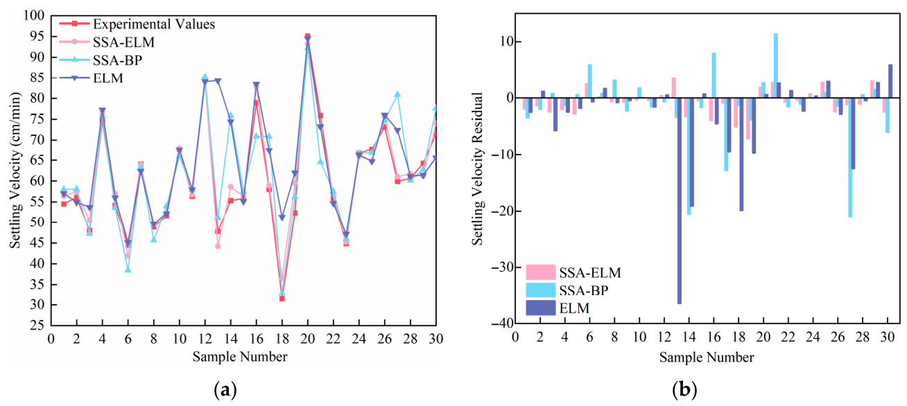
The predicted settling velocities are shown in Figure 4. As observed in Figure 4a, both the SSA-optimized BP and ELM models show better performance in predicting the settling velocity compared to the non-optimized ELM, with predictions closer to the experimental values. Moreover, the prediction trends of the optimized models align more closely with the actual variations, indicating that SSA optimization effectively enhances global search capability.

To directly compare the experimental and predicted values, the residual plot for each algorithm is presented in Figure 4b. Residuals represent the differences between the experimental and predicted values. As shown in Figure 4b, the ELM model exhibits the largest residuals, followed by SSA-BP, while SSA-ELM demonstrates the smallest residuals, suggesting its superior prediction performance.

To further quantify and compare prediction accuracy across models, commonly adopted error metrics and goodness-of-fit indicators were calculated and are presented in

Table 3. Performance metrics of different models for settling velocity prediction.

Evaluation Metric	SSA-ELM Model	SSA-BP Model	ELM Model
MAE	1.993 ± 0.092	2.921 ± 0.116	2.200 ± 0.356
MSE	6.432 ± 0.313	46.201 ± 2.557	36.923 ± 2.128
RMSE	2.536 ± 0.144	6.784 ± 0.451	6.076 ± 0.400
MAPE	3.613 ± 0.32	6.382 ± 0.665	10.216 ± 0.872
R2	0.960 ± 0.022	0.730 ± 0.031	0.490 ± 0.090

. MAE, MSE, RMSE and MAPE quantify the magnitude of discrepancy between predicted and actual values, with lower values indicating higher accuracy. The coefficient of determination, R², represents the proportion of variance explained by the model, ranging from 0 to 1, with a value closer to 1 indicating better predictive performance.

It can be seen from Table 3 that the quantitative metrics further confirm the superior prediction performance of SSA-ELM. Across all four error metrics, the SSA-ELM model yields the lowest values, indicating the smallest prediction deviations. Moreover, the R² value of SSA-ELM reaches 0.96, meaning that the model explains 96% of the variance in the settling velocity data, which is significantly higher than the 0.73 and 0.49 achieved by SSA-BP and ELM, respectively. The relatively poor performance of the standard ELM (R² = 0.49) can be attributed to its reliance on random initialization of input weights and hidden biases. Coal slime water settling is a highly nonlinear process governed by multiple interacting variables, and the underlying input-output relationship exhibits multiple local optima. For such a complex problem, random initialization often leads to suboptimal or locally optimal solutions without global optimization. In contrast, the SSA-optimized ELM performs a global search for optimal weights, effectively escaping poor local optima and achieving consistently high prediction accuracy, thereby demonstrating superior accuracy, robustness, and generalization for settling velocity prediction.

3.3.2. Prediction Performance of Supernatant Turbidity

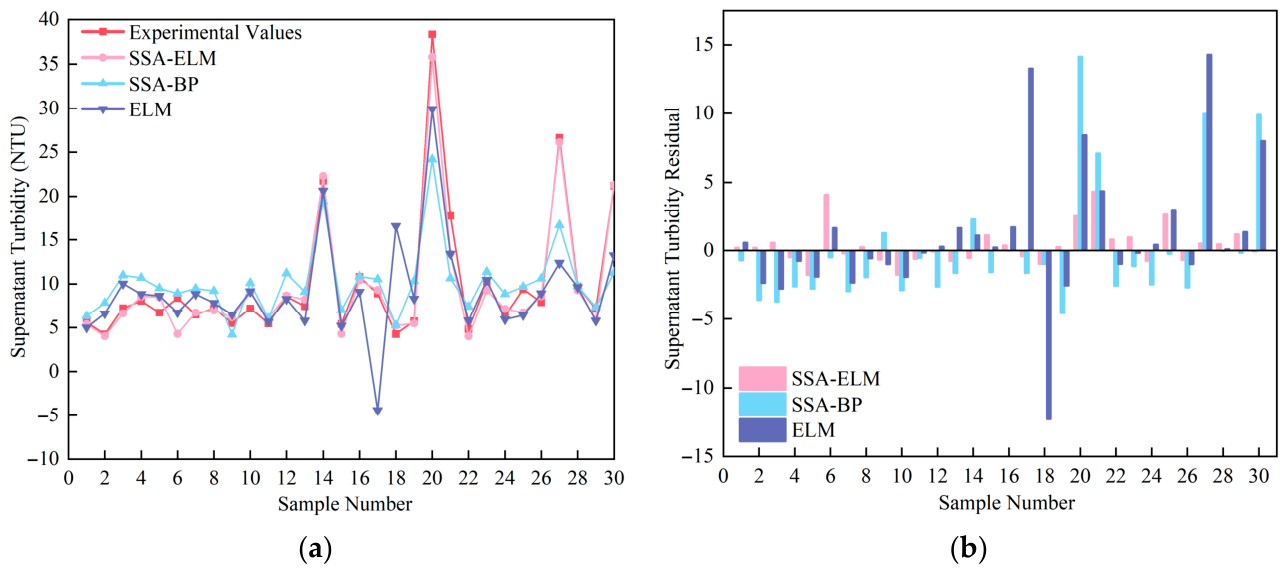
The three models were executed to predict the supernatant turbidity. The prediction results for the test set are shown in Figure 5a, with the corresponding residual plot presented in Figure 5b. The quantitative performance metrics are summarized in

Table 4. Performance metrics of different models for supernatant turbidity prediction.

Evaluation Metric	SSA-ELM Model	SSA-BP Model	ELM Model
MAE	1.023 ± 0.055	2.990 ± 0.137	1.308 ± 0.081
MSE	2.183 ± 0.126	19.257 ± 0.356	10.643 ± 0.288
RMSE	1.478 ± 0.061	4.389 ± 0.124	3.262 ± 0.117
MAPE	11.895 ± 0.369	26.870 ± 1.005	34.136 ± 1.654
R2	0.961 ± 0.030	0.650 ± 0.052	0.560 ± 0.120

.

As observed in Figure 5a, the overall prediction trend for supernatant turbidity remains most accurate with the SSA-ELM model. However, all three models show directional deviation from experimental values, which was not seen in the prediction of settling velocity. The performance variation across different outputs may stem from the complex coupling relationships among the four target parameters. The model’s attempt to reconcile potentially conflicting patterns during training could lead to compromised accuracy on individual targets, such as supernatant turbidity, a challenge compounded by the dataset’s wide yet sparse coverage and limited sample size.

Figure 5b indicates that for supernatant turbidity prediction, both the SSA-BP and ELM models show a wider range of residual variations, with most residual values higher than those of SSA-ELM, which aligns with the pattern observed in the previous subsection.

A comprehensive analysis of the metrics in Table 4 confirms that the SSA-ELM model delivers the best overall performance in predicting supernatant turbidity. Its R² value of 0.961 indicates that the model explains approximately 96% of the variance in the data, whereas the other two models explain only about 65% and 56%, respectively.

3.3.3. Prediction Performance of Sediment Layer Height

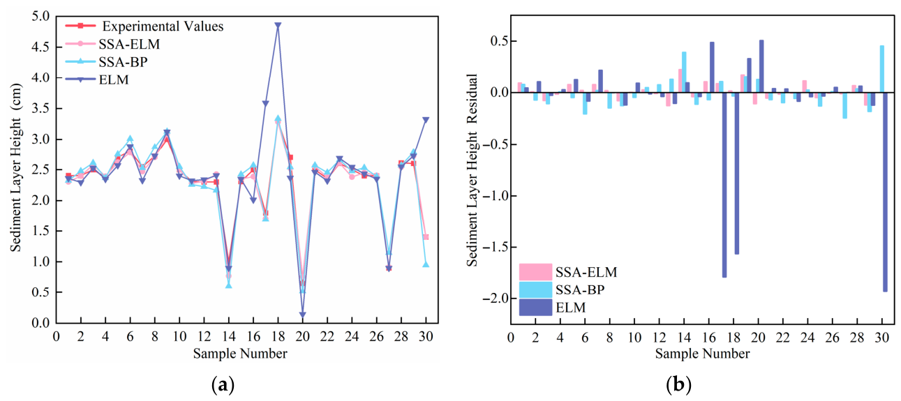
The three models were executed to predict the sediment layer height. The prediction results for the test set are shown in Figure 6a, with the corresponding residual plot presented in Figure 6b. The quantitative performance metrics are summarized in

Table 5. Performance metrics of different models for sediment layer height.

Evaluation Metric	SSA-ELM Model	SSA-BP Model	ELM Model
MAE	0.063 ± 0.005	0.116 ± 0.008	0.118 ± 0.009
MSE	0.007 ± 0.001	0.007 ± 0.002	0.145 ± 0.012
RMSE	0.084 ± 0.006	0.153 ± 0.010	0.380 ± 0.023
MAPE	3.421 ± 0.107	1.600 ± 0.082	15.504 ± 0.500
R2	0.980 ± 0.014	0.930 ± 0.013	0.120 ± 0.022

.

It can be seen from Figure 6a that all three models follow a similar overall trend for sediment layer height prediction. The prediction results of the two SSA-optimized models align more closely with the experimental values, whereas the standard ELM model produces several noticeable outliers. This discrepancy is primarily attributed to the weaker global search ability of standard ELM, hindering its convergence to an optimal solution.

As indicated in Figure 6b, the residuals of the SSA-optimized models remain low and exhibit very small fluctuation, while the ELM model shows significantly larger and more variable residuals.

The metrics given in Table 5 demonstrate that the two SSA-optimized models achieve very high accuracy in predicting sediment layer height. The SSA-ELM model obtains an R² of 0.98, explaining 98% variance of the data, while the SSA-BP model achieves an R² of 0.93. The superior performance of SSA-ELM over SSA-BP highlights the effectiveness of the SSA in fine-tuning the ELM’s parameters for enhanced local search and prediction precision. In contrast, the standard ELM model (R² = 0.12) fails to capture the underlying trend effectively.

3.3.4. Prediction Performance of Zeta Potential

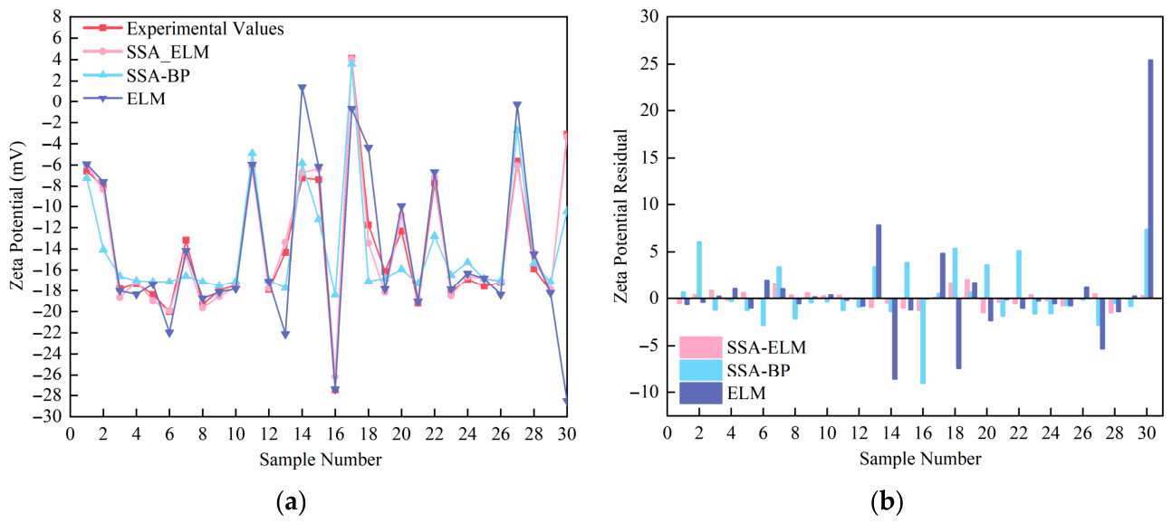
According to the DLVO theory [30], ζ potential governs the aggregation behavior of coal slime particles. Thus, the prediction and control of ζ potential are essential for optimizing the settling process. Given the current lack of solid in situ hardware-based measurement methods in industrial applications and limited prior research on its prediction, this study evaluates the predictive capability of three models for this key parameter. The models were executed, and their predictions for zeta potential are shown in Figure 7a, with the corresponding residual plot presented in Figure 7b. The quantitative performance metrics are summarized in

Table 6. Performance metrics of different models for zeta potential prediction.

Evaluation Metric	SSA-ELM Model	SSA-BP Model	ELM Model
MAE	0.649 ± 0.020	1.831 ± 0.051	1.123 ± 0.030
MSE	0.715 ± 0.023	10.658 ± 0.304	13.034 ± 0.466
RMSE	0.845 ± 0.017	3.265 ± 0.129	3.610 ± 0.151
MAPE	8.168 ± 0.316	20.450 ± 0.552	39.335 ± 1.331
R2	0.980 ± 0.005	0.740 ± 0.012	0.260 ± 0.020

.

The results from Figure 7a,b indicate that the SSA-ELM model achieves predictions highly consistent with the experimental values for $\zeta$ potential. In contrast, the other two models exhibit significantly larger and more variable residuals. The superior predictive accuracy and markedly lower errors of the SSA-ELM model indicate that it has captured the underlying relationship governing $\zeta$ potential more effectively than the benchmark models. This demonstrates its strong generalization capability and represents a substantial advance in predicting this critical parameter for the coal slime water settling process.

An analysis of Table 6 confirms that SSA-ELM delivers the best performance in predicting $\zeta$ potential, with an R² of 0.98. The SSA-BP and ELM models achieve substantially lower R² values of 0.74 and 0.26, respectively. For all the settling process parameters, the proposed SSA-ELM model is demonstrated to have the most robust and accurate prediction performance.

Furthermore, the computational efficiency of the three models was evaluated by recording the execution time. The SSA-BP model required 29.15 s, while the SSA-ELM and standard ELM models completed execution in 3.06 s and 0.59 s, respectively. This indicates that SSA-ELM not only offers superior prediction accuracy but also maintains a favorable computational speed. The excellent balance between prediction precision and computational cost makes SSA-ELM an ideal choice for modeling the settling process of coal slime water treatment.

4. Conclusions

In this study, a prediction model of essential coal slime water processing parameters was developed based on SSA-ELM. The model uses readily measurable inputs (coal slime water concentration, particle size distribution, water hardness, pH, and reagent dosage) to simultaneously achieve the “soft-sensor” of four settling process parameters: settling velocity, supernatant turbidity, sediment layer height, and the crucial $\zeta$ potential. This work provides a novel approach for predicting $\zeta$ potential, which is a determinant of particle aggregation and solid–liquid separation but difficult to measure in situ. The prediction performance of the proposed SSA-ELM model was thoroughly evaluated and compared against that of the standard ELM and SSA-BP model. The results demonstrate that the SSA-ELM model achieves the highest prediction accuracy for all four parameters, with R² values ranging from 0.95 to 0.98, outperforming previously reported soft-sensor models for coal slime water parameter prediction, while maintaining favorable computational efficiency (3.06 s). These findings confirm that SSA effectively enhances the global search capability and stability of ELM, making SSA-ELM a promising solution for predicting coal slime water settling parameters. This superior performance confirms that incorporating mechanism-based parameters (zeta potential) helps the model maintain high prediction accuracy even when operational conditions—such as solids concentration, water hardness, fines content, and pH—vary significantly. This capability provides a solid basis for upgrading existing industrial-scale intelligent dosing systems toward more robust, mechanism-driven control.

In summary, the findings of this work provide a foundation for mechanism-based dosing, directly contributing to improved efficiency, enhanced treatment outcomes, and reduced chemical costs. However, soft sensing of zeta potential is not a complete solution, as particle interactions in coal slime water are also governed by non-DLVO forces, particularly hydration forces, whose mechanistic origins and mathematical formulations remain incompletely understood. In highlighting the limitations of current approaches and the unresolved issues in extended DLVO theory, this work opens the door to a deeper integration of more comprehensive colloidal interaction mechanisms into predictive models—a direction that promises to advance the digital transformation of coal preparation plants toward smarter, truly mechanism-driven control.

References

1. Liu, X.; Yang, Y.; Zhao, Y. The path of coal to electricity revolution under the goals of carbon peak and carbon neutral. Min. Saf. Environ. Prot. 2024, 51, 14–18. [Google Scholar]
2. Schernikau, L. Economics of the International Coal Trade: Why Coal Continues to Power the World; Springer: Berlin/Heidelberg, Germany, 2017. [Google Scholar]
3. Coal’s Share in Global Generation Mix to Slip: IEA. Available online: https://www.argusmedia.com/en/news-and-insights/latest-market-news/2786338-coal-s-share-in-global-generation-mix-to-slip-iea (accessed on 10 January 2026).
4. Mao, X.; Liu, L. Present status of the research work on intelligent control in slime water treatment. Coal Prep. Technol. 2022, 50, 78–85. [Google Scholar]
5. Chen, D.; Liang, F.; Li, L.; Zhu, S.; Wang, X.; Bu, Q.; Chen, D.; Zhang, C. Study and application of the slime water system management and control technologies. Coal Prep. Technol. 2022, 50, 80–88. [Google Scholar]
6. Fan, Y.; Ruan, C.; Chang, M.; Dong, X.; Ma, X.; Ye, G. Effect of settling vortex of coal slime flocs with different sizes on the settlement of microfine particles. Powder Technol. 2025, 452, 120422. [Google Scholar] [CrossRef] [Scilit]
7. Zhang, B. Research and Application on Collaborative Control System of Medicament Accession of Concentration and Filtering Process. Master’s Thesis, Taiyuan University of Technology, Taiyuan, China, 2017. [Google Scholar]
8. Pan, F.; Ding, S.; Zou, H. Analysis of the Causes of Difficult Subsidence in Coal Slurry Water and Research Status of Treatment Technologies. Coal Process. Util. 2023, 3, 9–14. [Google Scholar]
9. Li, Q.; Liao, C.; Hou, J.; Wang, W.; Zhang, J. A mathematic model based on eDLVO and Lifshitz theory calculating interparticle interactions in coal water slurry. Fuel 2022, 316, 123271. [Google Scholar] [CrossRef] [Scilit]
10. Wang, Y.; Zhang, A. Analysis and Measurement of Slime Water with Difficult Subsidence in Coal Preparation Plant. Clean Coal Technol. 2018, 24, 130–133. [Google Scholar]
11. Liang, L.; Peng, Y.; Tan, J.; Xie, G. Intensified Ash Rejection in Coal Flotation by the Aggregation of Gangue Minerals Induced by Polyaluminum Chloride. Int. J. Coal Prep. Util. 2018, 38, 180–191. [Google Scholar] [CrossRef] [Scilit]
12. Shi, C.; Guo, D.; Li, Y.; Zhang, Z.; Tang, L. Effect of the Polymerized Titanium Ferric Sulfate (PTFS) Coagulant on Sedimentation of Coal Slime Water. Minerals 2022, 12, 26. [Google Scholar] [CrossRef] [Scilit]
13. Deng, J.; Liu, W.; Zheng, C.; Wang, C. Design and Application of the Intelligent Agent Dosing System in Coal Slurry Water Treatment Process at Buliangou Mine’s Coal Preparation Plant. Coal Prep. Technol. 2024, 52, 79–85. [Google Scholar]
14. Tao, Y.; Pan, Y. Study on the Intelligent Control System of Slime Water Dosing in Coal Preparation Plant. Clean Coal Technol. 2019, 25, 151–155. [Google Scholar]
15. Li, P.; Shen, Y.; Wang, X.; Song, Z.; Guo, J.; Qiao, P. Study and Application of the Intelligent Agent Dosing System in Coal Slurry Water Treatment Process. Coal Prep. Technol. 2024, 52, 79–86. [Google Scholar]
16. Yan, Y.; Tang, H.; Yu, F.; Huang, X. Research on Intelligent Dosing System for Coal Slurry Water in Limin Coal Preparation Plant. Coal Technol. 2023, 42, 258–261. [Google Scholar]
17. Wang, A. Research on Flocculation and Sedimentation Characteristics of Extremely Fine Coal Slime Based on Computer PID Algorithm. J. Phys. Conf. Ser. 2020, 1578, 012002. [Google Scholar] [CrossRef] [Scilit]
18. Dong, J.; Li, L.; Zhou, S.; Zhang, Y.; Wang, X. Research on Operation Test of XiaoJihan Coal Slurry Water Intelligent Dosing System. Shandong Chem. Ind. 2021, 50, 113–114, 118. [Google Scholar]
19. Xu, Z. Research and Application of Intelligent Agent Dosing System for Coal Slurry Water in Menkeqing Coal Preparation Plant. Coal Process. Util. 2022, 12, 9–13. [Google Scholar]
20. Wang, D.; Wang, C.; Liu, J.; Yuan, Y. Hybrid data and knowledge driven approach for determining coagulant dosing in drinking water treatment plants. Environ. Sci. Water Res. Technol. 2025, 11, 1770–1786. [Google Scholar] [CrossRef] [Scilit]
21. Yu, W.; Zhou, Z.; Yang, Y.; Li, X.; Lu, Z.; Liu, Y.; Ren, J.; Liu, Y. Artificial intelligence in chemical dosing for drinking water treatment: A systematic review of algorithmic applications, implementation frameworks, and future challenges. J. Environ. Chem. Eng. 2025, 13, 118936. [Google Scholar] [CrossRef] [Scilit]
22. Liu, F.; Ding, N.; Zheng, G.; Xu, J. Carbon emission prediction and reduction analysis of wastewater treatment plants based on hybrid machine learning models. Environ. Eng. Res. 2025, 30, 240403. [Google Scholar] [CrossRef] [Scilit]
23. Lu, X.; Huang, S.; Liu, H.; Yang, F.; Zhang, T.; Wan, X. Research on Intelligent Chemical Dosing System for Phosphorus Removal in Wastewater Treatment Plants. Water 2024, 16, 1623. [Google Scholar] [CrossRef] [Scilit]
24. Li, F.; Su, Z.; Wang, G.-m. An effective integrated control with intelligent optimization for wastewater treatment process. J. Ind. Inf. Integr. 2021, 24, 100237. [Google Scholar] [CrossRef] [Scilit]
25. Librantz, A.F.H.; dos Santos, F.C.R.; Dias, C.G. Artificial neural networks to control chlorine dosing in a water treatment plant. Acta Scientiarum. Technol. 2018, 40, e37275. [Google Scholar] [CrossRef] [Scilit]
26. Wang, D.; Li, S.; Zhou, X. Control-Oriented Modeling and Real-Time Control for the Ozone Dosing Process of Drinking Water Treatment. Environ. Sci. Technol. 2013, 47, 2197–2203. [Google Scholar] [CrossRef] [Scilit]
27. Zhang, Y.; Fan, Y.; Ma, X.; Dong, X.; Jin, W.; Wang, D. Prediction of Overflow Concentration of Thickener Based on ISSA-LSTM. J. Mine Autom. 2022, 48, 63–72. [Google Scholar]
28. Wu, T.W.R.; Wang, J. Research on Predictive Model of Thickener Slime Sedimentation Thickness Based on GSA-LSSVM. Coal Mine Mach. 2019, 40, 29–31. [Google Scholar]
29. Bello, O.; Hamam, Y.; Djouani, K. Control of a coagulation chemical dosing unit for water treatment plants using MMPC based on fuzzy weighting. J. Water Process Eng. 2014, 4, 34–46. [Google Scholar] [CrossRef] [Scilit]
30. Goddard, E.D. Foundations of colloid science: Vol. II, by Robert J. Hunter, Oxford University Press, 1991, 410 pp., ISBN 0-19-855392-7 (Pbk). Colloids Surf. A Physicochem. Eng. Asp. 1993, 74, 313. [Google Scholar] [CrossRef] [Scilit]
31. Israelachvili, J.N. Intermolecular and Surface Forces; Academic Press: Cambridge, MA, USA, 2011. [Google Scholar]
32. Ma, X. Study on the Adsorption Behavior of Solid-Liquid Separation Agent at the Interface of Coal Slurry. Ph.D. Thesis, Taiyuan University of Technology, Taiyuan, China, 2019. [Google Scholar]
33. Min, F.; Zhao, Q.; Li, H.; Peng, C. Study on Surface Charging Characteristics of Kaolin Particles in Coal Slurry Water. J. China Univ. Min. Technol. 2013, 42, 284–290. [Google Scholar]
34. Ding, H.; Tang, M.; Huang, Q.; Yang, P.; Liu, Z.; Bi, X.; Nair, A.; Wang, X. Soft sensor enabled real-time chemical dosing control systems for wastewater treatment: From hybrid model to full-scale application. J. Water Process Eng. 2024, 63, 105431. [Google Scholar] [CrossRef] [Scilit]
35. Shao, Q.; Wang, R. Prediction for Overflow Water Concentration of Concentrated Tank Based on PSO-LSSVM. China Coal 2017, 43, 117–120. [Google Scholar]
36. Wang, X.; Sun, T.; Gan, H.; Cao, Y.; Liu, F.; Qin, L. Research on Dosage Prediction of Coal Slurry Flotation Agent Based on PSO-ELM Algorithm. J. Yancheng Inst. Technol. (Nat. Sci. Ed.) 2024, 37, 26–30, 49. [Google Scholar]
37. Li, J.; Wu, Y. Improved Sparrow Search Algorithm with the Extreme Learning Machine and Its Application for Prediction. Neural Process. Lett. 2022, 54, 4189–4209. [Google Scholar] [CrossRef] [Scilit]
38. Xue, J.; Shen, B. A novel swarm intelligence optimization approach: Sparrow search algorithm. Syst. Sci. Control Eng. 2020, 8, 22–34. [Google Scholar] [CrossRef] [Scilit]
39. Yang, J.; Yang, J.; Wei, J.; Li, Q. Design of an Automatic Flocculant Dosing System Based on Grey Prediction-Fuzzy Control. J. Taiyuan Univ. Technol. 2012, 43, 606–609. [Google Scholar]
40. How to Proceed with the Intelligentization Construction of Coal Preparation Plants. Available online: https://mp.weixin.qq.com/s/kD4WiYD5LV1MrXn7WMg5gg (accessed on 23 March 2026).
41. MT/T 58-1993; Test Method for Sieve Analysis of Coal Powder. Coal Industry Press: Beijing, China, 1993.
42. MT 190-1988; Test Method for Settling of Coal Slurry Water in Coal Preparation Plants. Coal Industry Press: Beijing, China, 1988.
43. Shao, W.; Ge, Z.; Song, Z.; Wang, K. Nonlinear industrial soft sensor development based on semi-supervised probabilistic mixture of extreme learning machines. Control Eng. Pract. 2019, 91, 104098. [Google Scholar] [CrossRef] [Scilit]
44. Ooi, B.P.; Rahim, N.A.; Masnan, M.J.; Zakaria, A. A study of extreme learning machine on small sample-sized classification problems. J. Phys. Conf. Ser. 2021, 2107, 012013. [Google Scholar] [CrossRef] [Scilit]
45. Yu, L.; Zhang, X.; Yin, H. An extreme learning machine based virtual sample generation method with feature engineering for credit risk assessment with data scarcity. Expert Syst. Appl. 2022, 202, 117363. [Google Scholar] [CrossRef] [Scilit]
46. Alnagashi, F.A.K.Q.; Rahim, N.A.; Shukor, S.A.A.; Hamid, M.H.A. Mitigating overfitting in extreme learning machine classifier through dropout regularization. Appl. Math. Comput. Intell. (AMCI) 2024, 13, 26–35. [Google Scholar] [CrossRef] [Scilit]
47. Samat, A.; Du, P.; Liu, S.; Li, J.; Cheng, L. Ensemble Extreme Learning Machines for Hyperspectral Image Classification. IEEE J. Sel. Top. Appl. Earth Obs. Remote Sens. 2014, 7, 1060–1069. [Google Scholar] [CrossRef] [Scilit]
48. Huang, G.-B.; Zhu, Q.-Y.; Siew, C.-K. Extreme learning machine: Theory and applications. Neurocomputing 2006, 70, 489–501. [Google Scholar] [CrossRef] [Scilit]
49. Zhang, R.; Deng, Z.; Wang, S.; Choi, K.; Qian, P. Robust single hidden layer feed-forward neural networks modeling forsmall datasets. Control Decis. 2012, 27, 1308–1312+1319. [Google Scholar]
50. Xie, Q.; Tian, Q. Extreme Nonlinear Discriminant Analysis Network with Random Orthogonalization of Weights. Comput. Technol. Dev. 2018, 28, 23–27. [Google Scholar]
51. Du, Y.; Zhou, Z.; Jia, K.; Ding, L.; Lu, M. Chaotic Sparrow Search Algorithm with Hybrid Multiple Adaptive Weights. Comput. Eng. Appl. 2024, 60, 70–83. [Google Scholar]
52. Biswas, M.; Shome, A.; Islam, M.A.; Nova, A.J.; Ahmed, S. Predicting stock market price: A logical strategy using deep learning. In Proceedings of 2021 IEEE 11th IEEE Symposium on Computer Applications & Industrial Electronics (ISCAIE); IEEE: Piscataway, NJ, USA, 2021; pp. 218–223. [Google Scholar]
53. Rodrigues, C.H.; Pires, D.E.; Ascher, D.B. DynaMut: Predicting the impact of mutations on protein conformation, flexibility and stability. Nucleic Acids Res. 2018, 46, W350–W355. [Google Scholar] [CrossRef] [Scilit] [PubMed]
54. Eldar, Y.C.; Nehorai, A.; La Rosa, P.S. A competitive mean-squared error approach to beamforming. IEEE Trans. Signal Process. 2007, 55, 5143–5154. [Google Scholar] [CrossRef]
55. Xu, Q.-S.; Liang, Y.-Z. Monte Carlo cross validation. Chemom. Intell. Lab. Syst. 2001, 56, 1–11. [Google Scholar] [CrossRef] [Scilit]
56. Shan, G. Monte Carlo cross-validation for a study with binary outcome and limited sample size. BMC Med. Inform. Decis. Mak. 2022, 22, 270. [Google Scholar] [CrossRef] [Scilit]
57. Wang, Z.; Dai, H.; Chen, B.; Cheng, S.; Sun, Y.; Zhao, J.; Guo, Z.; Cai, X.; Wang, X.; Li, B.; et al. Effluent quality prediction of the sewage treatment based on a hybrid neural network model: Comparison and application. J. Environ. Manag. 2024, 351, 119900. [Google Scholar] [CrossRef] [Scilit]
58. Ling, G.; Wang, Z.; Shi, Y.; Wang, J.; Lu, Y.; Li, L. Membrane Fouling Prediction Based on Tent-SSA-BP. Membranes 2022, 12, 691. [Google Scholar] [CrossRef] [Scilit] [PubMed]
59. Yan, L.; Englert, A.H.; Masliyah, J.H.; Xu, Z. Determination of Anisotropic Surface Characteristics of Different Phyllosilicates by Direct Force Measurements. Langmuir 2011, 27, 12996–13007. [Google Scholar] [CrossRef] [Scilit]
60. Chang, J.; Shao, H.; Liu, B.; Manica, R.; Li, Z.; Liu, Q.; Xu, Z. Control of nanostructures through pH-dependent self-assembly of nanoplatelets. J. Colloid Interface Sci. 2021, 582, 439–445. [Google Scholar] [CrossRef] [Scilit] [PubMed]
61. Darbha, G.K.; Schäfer, T.; Heberling, F.; Lüttge, A.; Fischer, C. Retention of Latex Colloids on Calcite as a Function of Surface Roughness and Topography. Langmuir 2010, 26, 4743–4752. [Google Scholar] [CrossRef] [Scilit] [PubMed]
62. Yan, L.; Masliyah, J.H.; Xu, Z. Understanding suspension rheology of anisotropically-charged platy minerals from direct interaction force measurement using AFM. Curr. Opin. Colloid Interface Sci. 2013, 18, 149–156. [Google Scholar] [CrossRef] [Scilit]
63. Song, Z.; Li, Y. Water Pollution Control Engineering, 2nd ed.; China University of Mining and Technology Press: Xuzhou, China, 2019. [Google Scholar]
Figure 1. ELM Topology Diagram.
Separations 13 00115 g001
Figure 2. SSA-ELM model construction flowchart.
Separations 13 00115 g002
Figure 3. XRD diffractogram for mineral composition analysis of the coal slime sample.
Separations 13 00115 g003
Figure 4. Prediction results and validation for settling velocity. (a) Model outputs versus experimental data; (b) corresponding residuals.
Separations 13 00115 g004
Figure 5. Prediction results and validation for supernatant turbidity. (a) Model outputs versus experimental data; (b) Corresponding residuals.
Separations 13 00115 g005
Figure 6. Prediction results and validation for sediment layer height. (a) Model outputs versus experimental data; (b) Corresponding residuals.
Separations 13 00115 g006
Figure 7. Prediction results and validation for zeta (ζ) potential. (a) Model outputs versus experimental data; (b) Corresponding residuals.
Separations 13 00115 g007