Economic Dispatch of Multi-Energy System Considering Load Replaceability

Abstract
:1. Introduction
2. Load Replaceability in Multi-Energy System
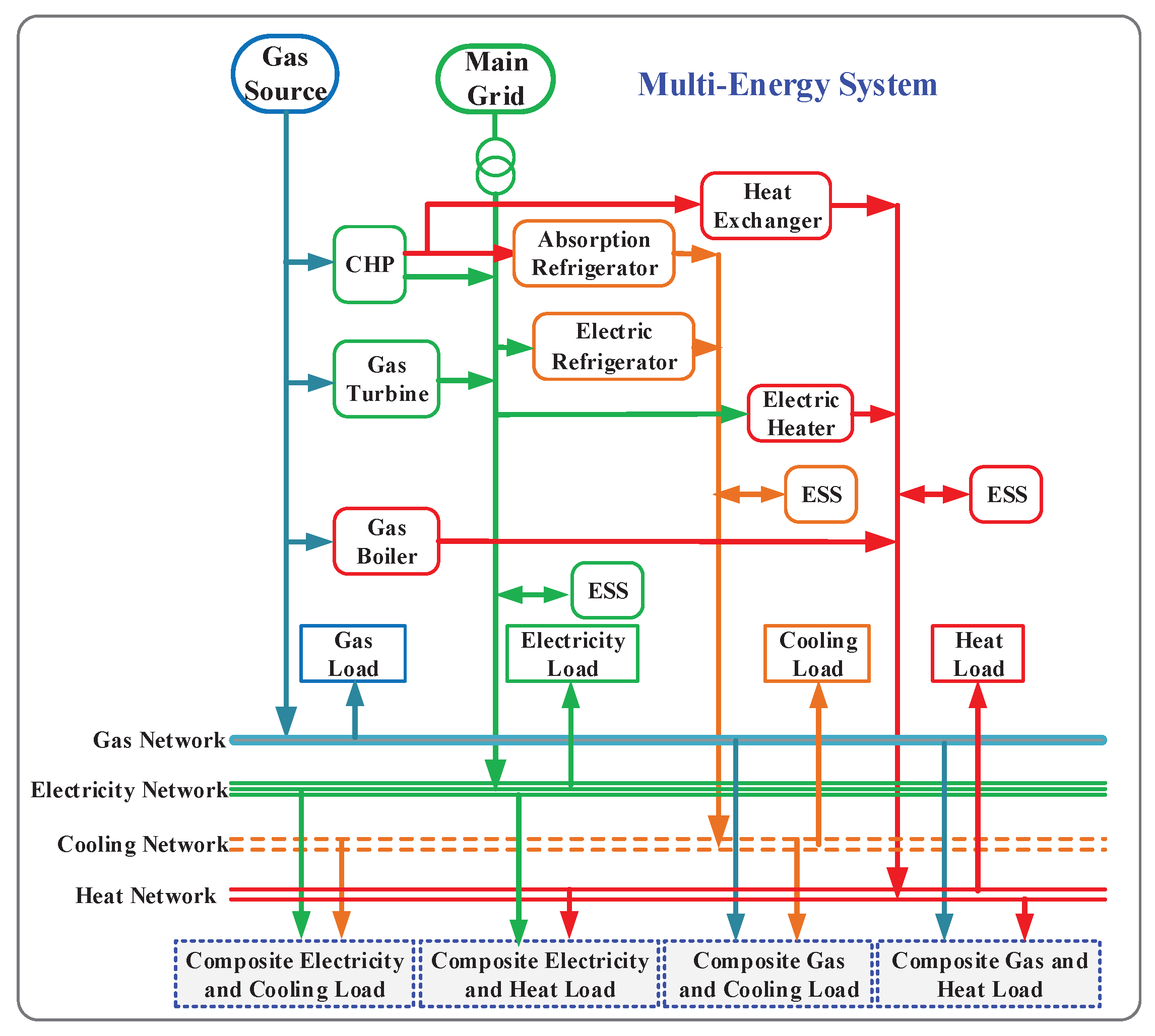
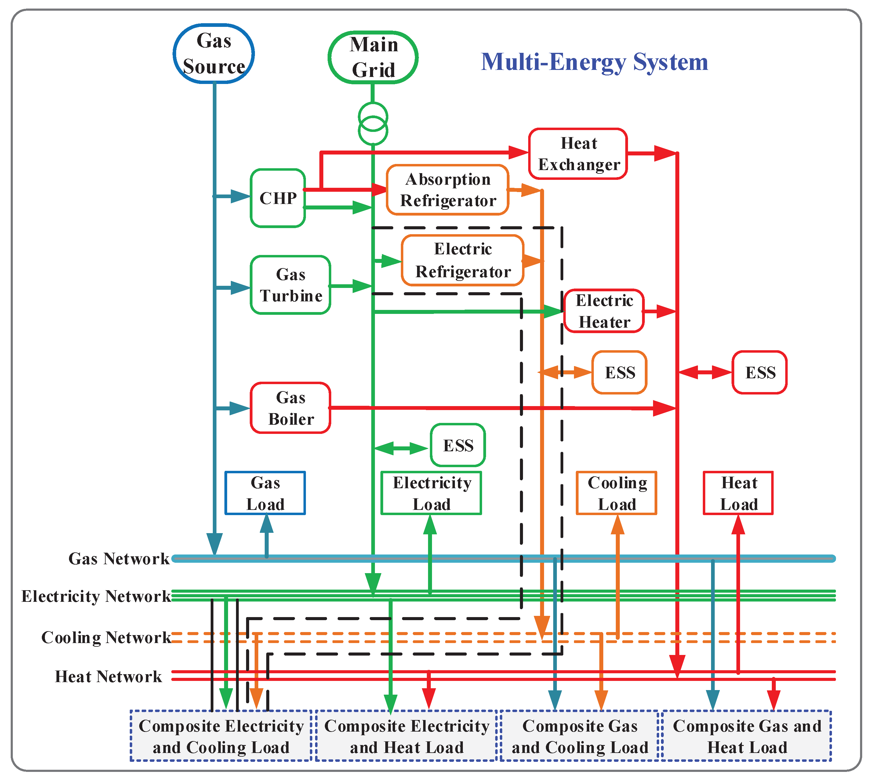
2.1. Load Replaceability and Composite Load
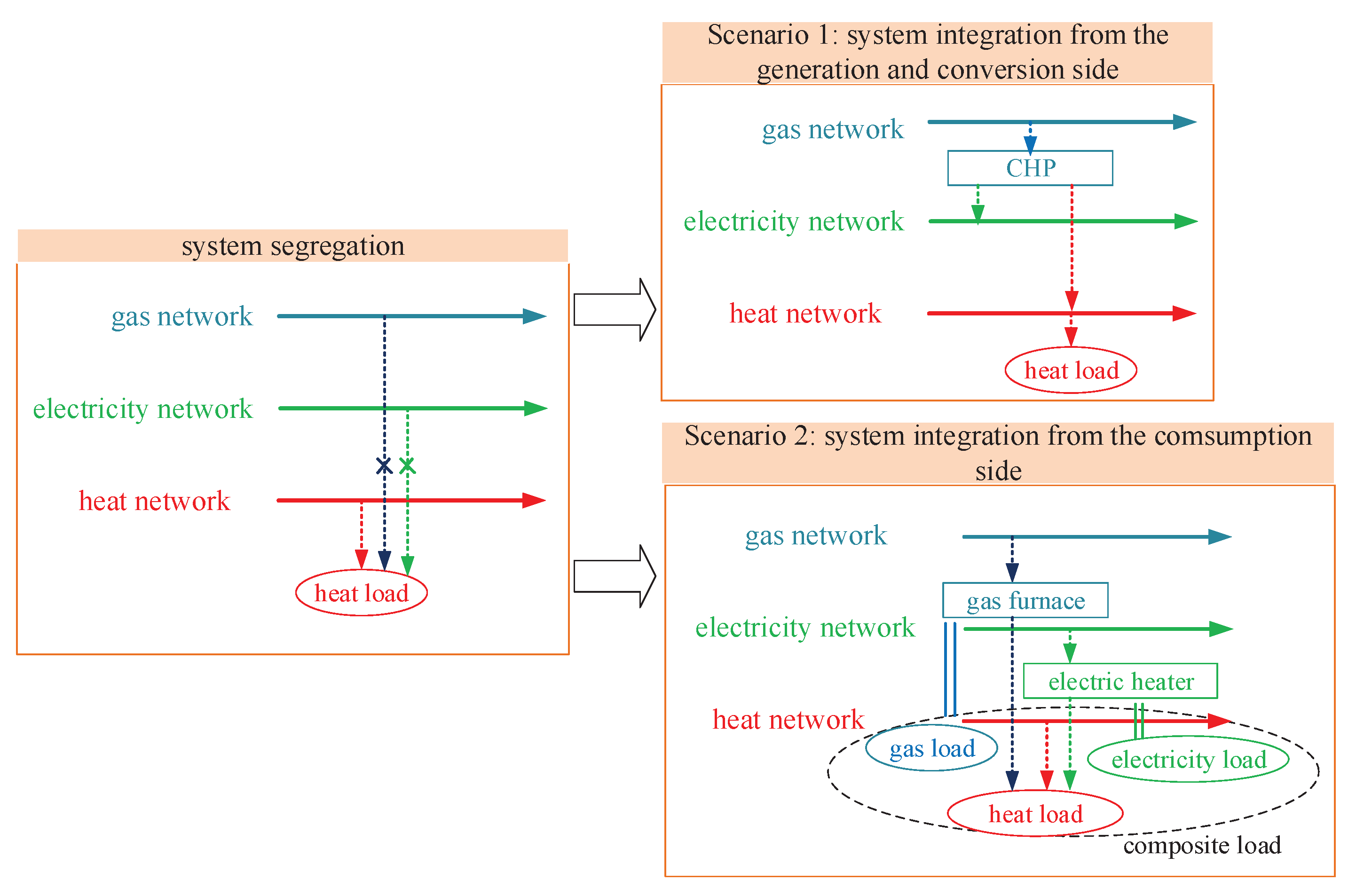
- Scenario 1: There exists no replaceable heat load in the system; the multi-generation plant is the CHP plant. The overall energy conversion ratio is 0.8; the energy proportion of electricity generated by the CHP plant is 0.6; the energy proportion of heat generated by the CHP plant is 0.4. And the maximal capacity of the CHP plant is supposedly to be much bigger than the maximal transmission capacity of the network.
- Scenario 2: There exists replaceable heat load in the system, and the load is composite load which contains electric heater and gas furnace. The maximal capacity of both devices is supposedly to be much bigger than the maximal transmission capacity of power and gas network. The energy efficiency ratio for both devices is 0.5.
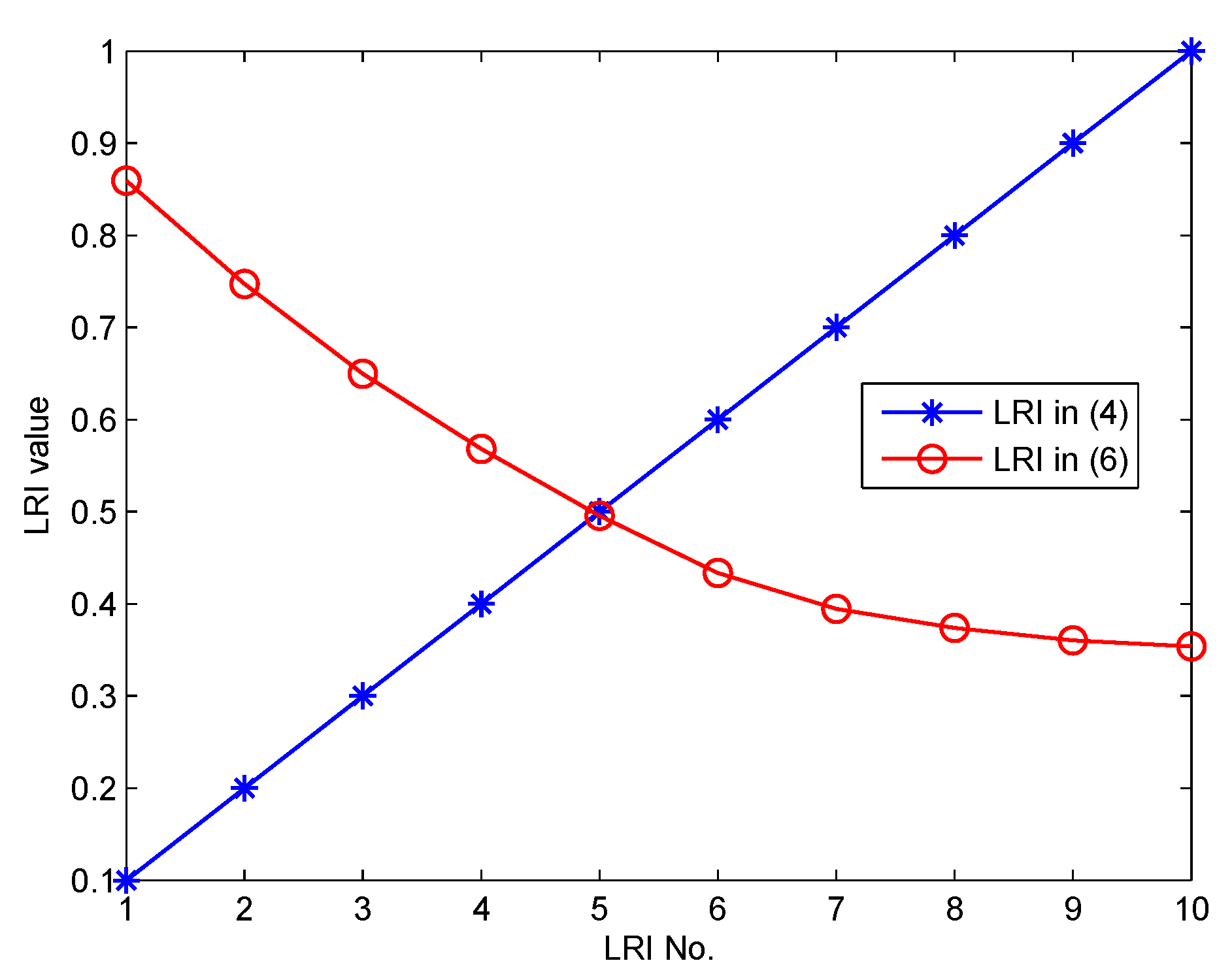
2.2. Load Replaceability Index
2.2.1. Load Replaceability Index Reflecting Potential Load Substitution Ability
2.2.2. Load Replaceability Index Reflecting Actual Load Substitution Ability
3. Optimal Economic Scheduling of Multi-Energy System Considering Load Replaceability
3.1. Objective Function of Optimal Economic Scheduling of MES
3.2. Constraints of Optimal Economic Scheduling of MES
3.2.1. Energy Supply and Demand Balance
3.2.2. Energy Balance of Conversion Systems
3.2.3. Energy Storage Systems
3.2.4. Other Constraints
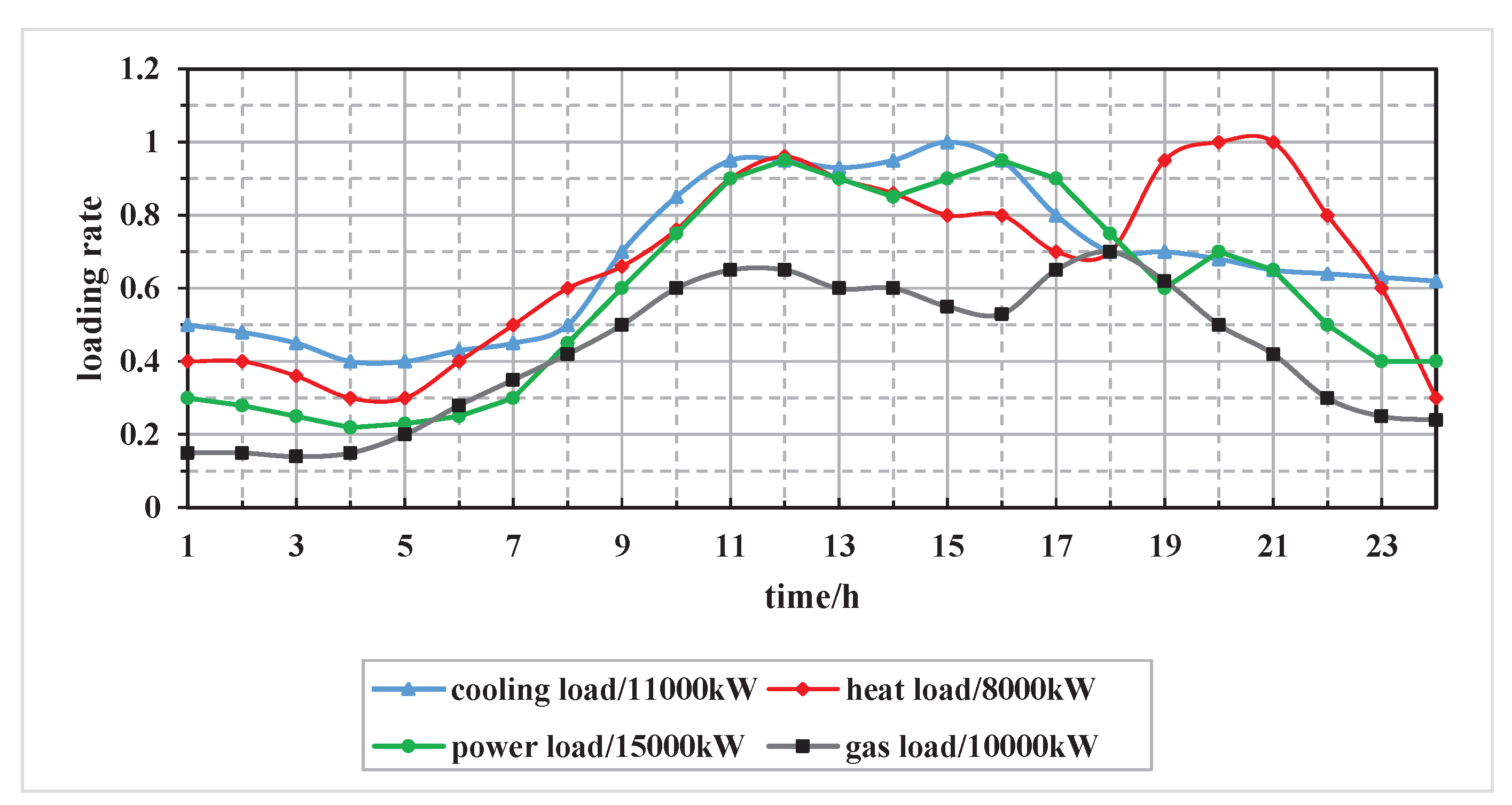
4. Case Study
4.1. Simulation Settings
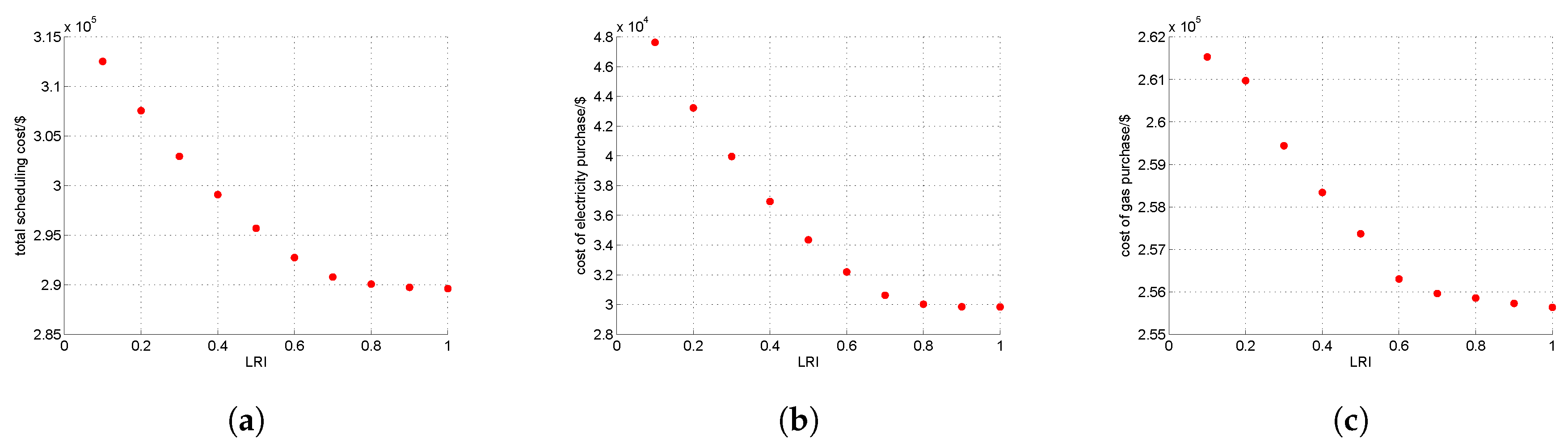
4.2. Simulation Results and Discussions
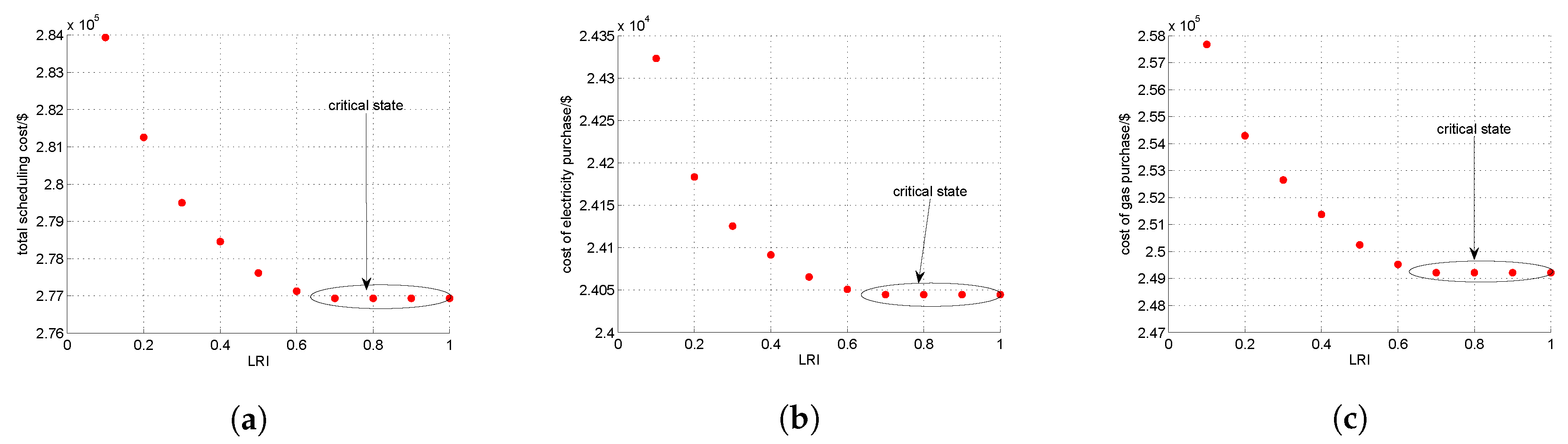
4.2.1. Scenario 1
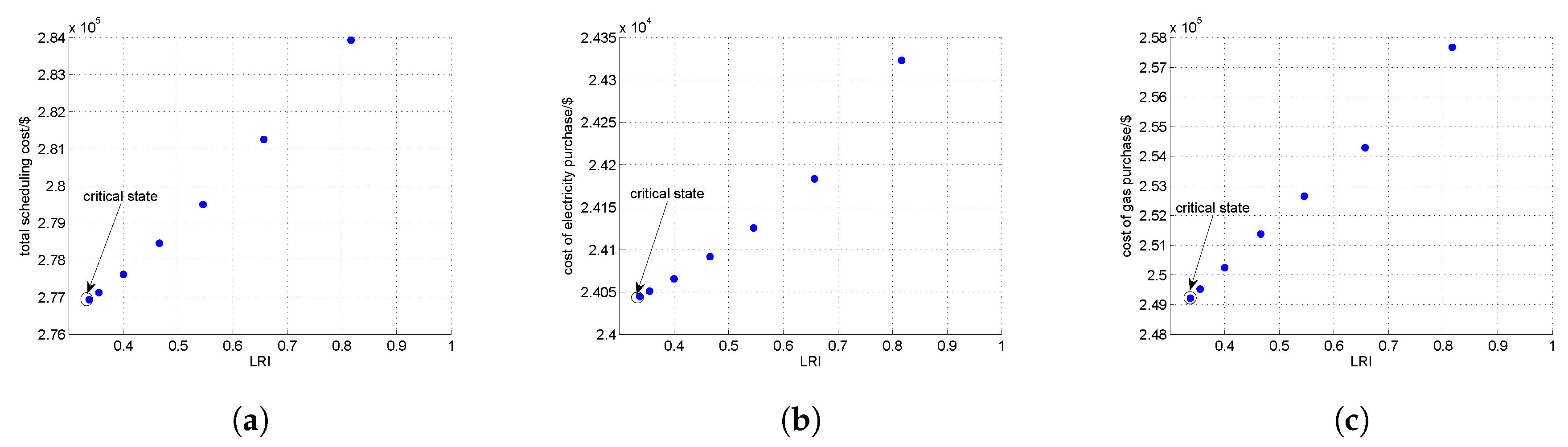
4.2.2. Scenario 2
5. Conclusions
Author Contributions
Funding
Conflicts of Interest
References
- Vasebi, A.; Fesanghary, M.; Bathaee, S. Combined heat and power economic dispatch by harmony search algorithm. Int. J. Electr. Power Energy Syst. 2007, 29, 713–719. [Google Scholar] [CrossRef]
- Vögelin, P.; Koch, B.; Georges, G.; Boulouchos, K. Heuristic approach for the economic optimisation of combined heat and power (CHP) plants: Operating strategy, heat storage and power. Energy 2017, 121, 66–77. [Google Scholar] [CrossRef]
- Wu, C.; Jiang, P.; Sun, Y.; Zhang, C.; Gu, W. Economic dispatch with chp and wind power using probabilistic sequence theory and hybrid heuristic algorithm. J. Renew. Sustain. Energy 2017, 9, 013303. [Google Scholar] [CrossRef]
- Li, Z.; Wu, W.; Shahidehpour, M.; Wang, J.; Zhang, B. Combined heat and power dispatch considering pipeline energy storage of district heating network. IEEE Trans. Sustain. Energy 2015, 7, 12–22. [Google Scholar] [CrossRef]
- Hashemi, R. A developed offline model for optimal operation of combined heating and cooling and power systems. IEEE Trans. Energy Convers. 2009, 24, 222–229. [Google Scholar] [CrossRef]
- Facci, A.L.; Andreassi, L.; Ubertini, S. Optimization of CHCP (combined heat power and cooling) systems operation strategy using dynamic programming. Energy 2014, 66, 387–400. [Google Scholar] [CrossRef]
- Li, M.; Mu, H.; Li, N. Optimal design and operation strategy for integrated evaluation of CCHP (combined cooling heating and power) system. Energy 2016, 99, 202–220. [Google Scholar] [CrossRef]
- Tan, Z.; Guo, H.; Lin, H.; Tan, Q.; Yang, S.; Gejirifu, D.; Ju, L.; Song, X. Robust scheduling optimization model for multi-energy interdependent system based on energy storage technology and ground-source heat pump. Processes 2019, 7, 27. [Google Scholar] [CrossRef]
- Wang, M.; Wang, J.; Zhao, P.; Dai, Y. Multi-objective optimization of a combined cooling, heating and power system driven by solar energy. Energy Convers. Manag. 2015, 89, 289–297. [Google Scholar] [CrossRef]
- Motevasel, M.; Seifi, A.R.; Niknam, T. Multi-objective energy management of CHP (combined heat and power)-based micro-grid. Energy 2013, 51, 123–136. [Google Scholar] [CrossRef]
- Li, K.; Yan, H.; He, G.; Zhu, C.; Liu, K.; Liu, Y. Seasonal Operation Strategy Optimization for Integrated Energy Systems with Considering System Cooling Loads Independently. Processes 2018, 6, 202. [Google Scholar] [CrossRef]
- Zhang, X.; Shahidehpour, M.; Alabdulwahab, A.; Abusorrah, A. Optimal expansion planning of energy hub with multiple energy infrastructures. IEEE Trans. Smart Grid 2015, 6, 2302–2311. [Google Scholar] [CrossRef]
- Parisio, A.; Del Vecchio, C.; Vaccaro, A. A robust optimization approach to energy hub management. Int. J. Electr. Power Energy Syst. 2012, 42, 98–104. [Google Scholar] [CrossRef]
- Vahid-Pakdel, M.; Nojavan, S.; Mohammadi-Ivatloo, B.; Zare, K. Stochastic optimization of energy hub operation with consideration of thermal energy market and demand response. Energy Convers. Manag. 2017, 145, 117–128. [Google Scholar] [CrossRef]
- Huang, Y.; Zhang, W.; Yang, K.; Hou, W.; Huang, Y. An optimal scheduling method for multi-energy hub systems using game theory. Energies 2019, 12, 2270. [Google Scholar] [CrossRef]
- Lin, Y.; Chen, B.; Wang, J.; Bie, Z. A combined repair crew dispatch problem for resilient electric and natural gas system considering reconfiguration and DG islanding. IEEE Trans. Power Syst. 2019, 34, 2755–2767. [Google Scholar] [CrossRef]
- Liu, Z.; Yang, P.; Xu, Z. Capacity allocation of integrated energy system considering typical day economic operation. Electr. Power Constr. 2017, 38, 51–59. [Google Scholar]
- Zhao, F.; Sun, B.; Zhang, C. Cooling, heating and electrical load forecasting method for CCHP system based on multivariate phase space reconstruction and Kalman filter. Proc. CSEE 2016, 36, 399–406. [Google Scholar]
- Chen, F.; Xu, J.; Wang, C. Research on building cooling and heating load prediction model on user’s side in energy internet system. Proc. CSEE 2015, 35, 3678–3684. [Google Scholar]
- Shi, J.; Tan, T.; Guo, J. Multi-task learning based on deep architecture for various types of load forecasting in regional energy system integration. Power Syst. Technol. 2018, 42, 698–706. [Google Scholar]
- Sheikhi, A.; Rayati, M.; Bahrami, S. Integrated demand side management game in smart energy hubs. IEEE Trans. Smart Grid 2015, 6, 675–683. [Google Scholar] [CrossRef]
- Bahrami, S.; Sheikhi, A. From demand response in smart grid toward integrated demand response in smart energy hub. IEEE Trans. Smart Grid 2016, 7, 650–658. [Google Scholar] [CrossRef]


| Parameter | Value |
|---|---|
| maximum allowable electricity procurement | 12,000 kW |
| maximum allowable gas procurement | 60,000 kW |
| maximum output of electric heater | 2000 kW |
| maximum output of electric refrigerator | 2000 kW |
| maximum output electricity of CHP plant | 8000 kW |
| maximum output of heat exchanger | 4000 kW |
| maximum output of absorption refrigerator | 6000 kW |
| maximum output of gas boiler | 2000 kW |
| maximum output of gas turbine | 8000 kW |
| power generation efficiency of CHP plant | 0.3 |
| electricity-to-heat ratio of CHP plant | 2/3 |
| energy efficiency ratio of heat exchanger | 0.9 |
| energy efficiency ratio of absorption refrigerator | 0.9 |
| energy efficiency ratio of electric heater | 0.95 |
| energy generation proportion ratio | 0.6 |
| energy efficiency ratio of electric refrigerator | 3.5 |
| energy efficiency ratio of gas boiler | 0.9 |
| maximum charge/discharge energy of electricity ESS | 2000 kW |
| maximum charge/discharge energy of heat ESS | 1000 kW |
| maximum charge/discharge energy of cooling ESS | 2000 kW |
| maximum remaining energy of electricity ESS | 8000 kWh |
| maximum remaining energy of heat ESS | 4000 kWh |
| maximum remaining energy of cooling ESS | 8000 kWh |
| attrition rate of electricity ESS | 0.2% |
| attrition rate of heat ESS | 0.3% |
| attrition rate of cooling ESS | 0.2% |
| operating cost of electricity ESS | 0.32 $/kWh |
| operating cost of heat ESS | 0.25 $/kWh |
| operating cost of cooling ESS | 0.2 $/kWh |
| Periods | Periods | ||
|---|---|---|---|
| 00:00–07:00 | 2.7 | 00:00–08:00 | 0.35 |
| 07:00–12:00 | 3.3 | 08:00–12:00 | 1.65 |
| 12:00–16:00 | 3.0 | 12:00–17:00 | 0.95 |
| 16:00–20:00 | 3.3 | 17:00–21:00 | 1.65 |
| 20:00–24:00 | 3.0 | 21:00–24:00 | 0.95 |
© 2019 by the authors. Licensee MDPI, Basel, Switzerland. This article is an open access article distributed under the terms and conditions of the Creative Commons Attribution (CC BY) license (http://creativecommons.org/licenses/by/4.0/).
Share and Cite
Zheng, T.; Dai, Z.; Yao, J.; Yang, Y.; Cao, J. Economic Dispatch of Multi-Energy System Considering Load Replaceability. Processes 2019, 7, 570. https://doi.org/10.3390/pr7090570
Zheng T, Dai Z, Yao J, Yang Y, Cao J. Economic Dispatch of Multi-Energy System Considering Load Replaceability. Processes. 2019; 7(9):570. https://doi.org/10.3390/pr7090570
Chicago/Turabian StyleZheng, Tao, Zemei Dai, Jiahao Yao, Yufeng Yang, and Jing Cao. 2019. "Economic Dispatch of Multi-Energy System Considering Load Replaceability" Processes 7, no. 9: 570. https://doi.org/10.3390/pr7090570
APA StyleZheng, T., Dai, Z., Yao, J., Yang, Y., & Cao, J. (2019). Economic Dispatch of Multi-Energy System Considering Load Replaceability. Processes, 7(9), 570. https://doi.org/10.3390/pr7090570