Monitoring and Analysis of Wave Characteristics during Pipeline End Termination Installation

Abstract

Pipeline end termination (PLET) installation is an essential part of offshore pipe-laying operation. Pipe-laying operations are sensitive to pipe-laying barge motion and marine environmental conditions. Monitoring the field environment can provide a reasonable basis for planning pipe-laying. Therefore, the measurement and analysis of sea wave motion is helpful for the control and operational safety of the pipeline and vessels. In this study, an environmental monitoring system was established to measure wave motion during PLET operation. Fourier transforms were used to process images that were acquired by ultra-high-frequency X-band marine radar to extract wave parameters. The resulting wave spectra, as measured each minute, were used to simulate real-time wave data and calculate wave characteristics and regressed wave frequency and direction spectrum throughout the PLET operation. The regressed frequency, spectral density, and direction spectra were compared with the theoretical spectra to evaluate their similarity and find the most similar spreading function in the operational area (the South China Sea). Gaussian fitting of real-time wave data was tested while using a classical method. The marginal distribution and joint density of the wave characteristics were estimated and then compared with theoretical distributions to find the most suitable model for improving marine environmental forecasting.

1. Introduction

Information on changes in sea conditions is essential for marine activities, including offshore operation activities, fisheries, marine resource transformations, and deep-sea development. The challenges for offshore engineering constantly change with the continuous development of deep water and open sea areas. The operating speed and precision for installing pipelines and other deep-sea equipment need to constantly improve to adapt to increasing developmental requirements [1,2]. Vessel motion and installation are highly sensitive to environmental changes during pipeline installation [3,4]. It is essential to acquire a better understanding of the marine environment during installation to provide these operations with higher accuracy, which can significantly help with planning pipeline installation.

There are many approaches for monitoring offshore engineering operations in pipeline installation [5]. To conduct such operations and expertly and securely install a pipeline, a system for monitoring the ocean environment while laying an offshore pipeline has been developed that measures vessel motion, position, heading profile, and top tension [6]. This monitoring system has achieved full-time tracking of the pipe-laying process and other functions, such as the touch-down point and pipeline fatigue. However, the system mainly monitors vessel motion and pipeline fatigue and thus neglects marine environmental analysis for installation operations, which can provide a basis for safety assessments and sea state forecasts. Another monitoring system that is used for floatover installations includes environmental and position monitoring functions to validate the installation tests and calibrate the monitoring system [7]. However, these monitoring systems do not acquire detailed measurements of specific wave parameters; thus, there is no analysis or induction of the wave characteristics.

Recent research in marine environmental monitoring has paid more attention to specific sea areas for longer periods of time to obtain reliable information [8]. The development of better wave observation technologies in recent years has yielded a greater variety of wave measurement devices, such as buoys, wave gages, and sensors, including radar sensors [9,10]. A home-made buoy-type wave height meter was used to perform measurements off the shore of northern China [11]. While using offshore buoy observations along the California coast, O’Reilly showed that buoy-driven model hindcasts have low bias and they are suitable for predicting mean wave climate conditions [12]. Additional shallow water wave height measurements were performed while using a cable-type wave monitoring system; however, these wave height observations were discontinuous, and the algorithm was only applicable to an inner space of less than 100 m [13]. An operational wave monitoring system was used for a Mediterranean beach to predict the wave evolution up to five days in advance by running the system once a day [14]. A regional coastal ocean observation system was also built for wave measurements [15]. Yasukuni Mori first presented measurements from light-emitting diode radar to monitor waves and evaluate the relationship between the wind and the waves [16]. Carrasco and Seeman measured the surface wave properties and spectral parameters while using Doppler marine radar [17].

Real-time wave monitoring systems were used to measure continuous wave data, and the acquired data were then used to calculate other environmental properties, such as wind speed and surface current direction [18,19,20]. For the total monitoring of marine environmental parameters, a semi-enclosed basin-monitoring system was designed to show the annual evolution of the measured parameters in the area investigated [21]. However, these wave monitoring systems were built to measure certain marine parameters and they do not provide a precise description of the sea conditions for specific engineering operations, even though these operations are susceptible to the sea level. In addition, the theoretical spectrum and corresponding environmental parameters were obtained by regressing a wave spectrum while using the measured data to provide an environmental reference for offshore engineering.

It is necessary to analyze the wave characteristics of the laying process and other working conditions of the pipeline to determine the working environmental parameters during pipe-laying operations with a lay-barge. This study aims to present and discuss real-time and continuous recording of marine environmental data that were collected using X-band radar in the South China Sea during a pipeline end termination (PLET) installation. Two frequency spectra were regressed while using real-time wave data that were simulated using a spectrum that was measured every minute by radar during the entire PLET installation. The regressed frequency spectra were compared with theoretical ocean spectra, and the direction spectra were compared with the theoretical spreading functions. The wave characteristics were analyzed while using the regressed spectra, including the marginal distribution of the wave characteristics, the joint distribution of the local wave maxima and minima, and the joint distribution of the wave height and period. This was to understand the waves during PLET installation and to provide a design basis for PLET installation operations and other offshore engineering projects.

2. Materials and Methods

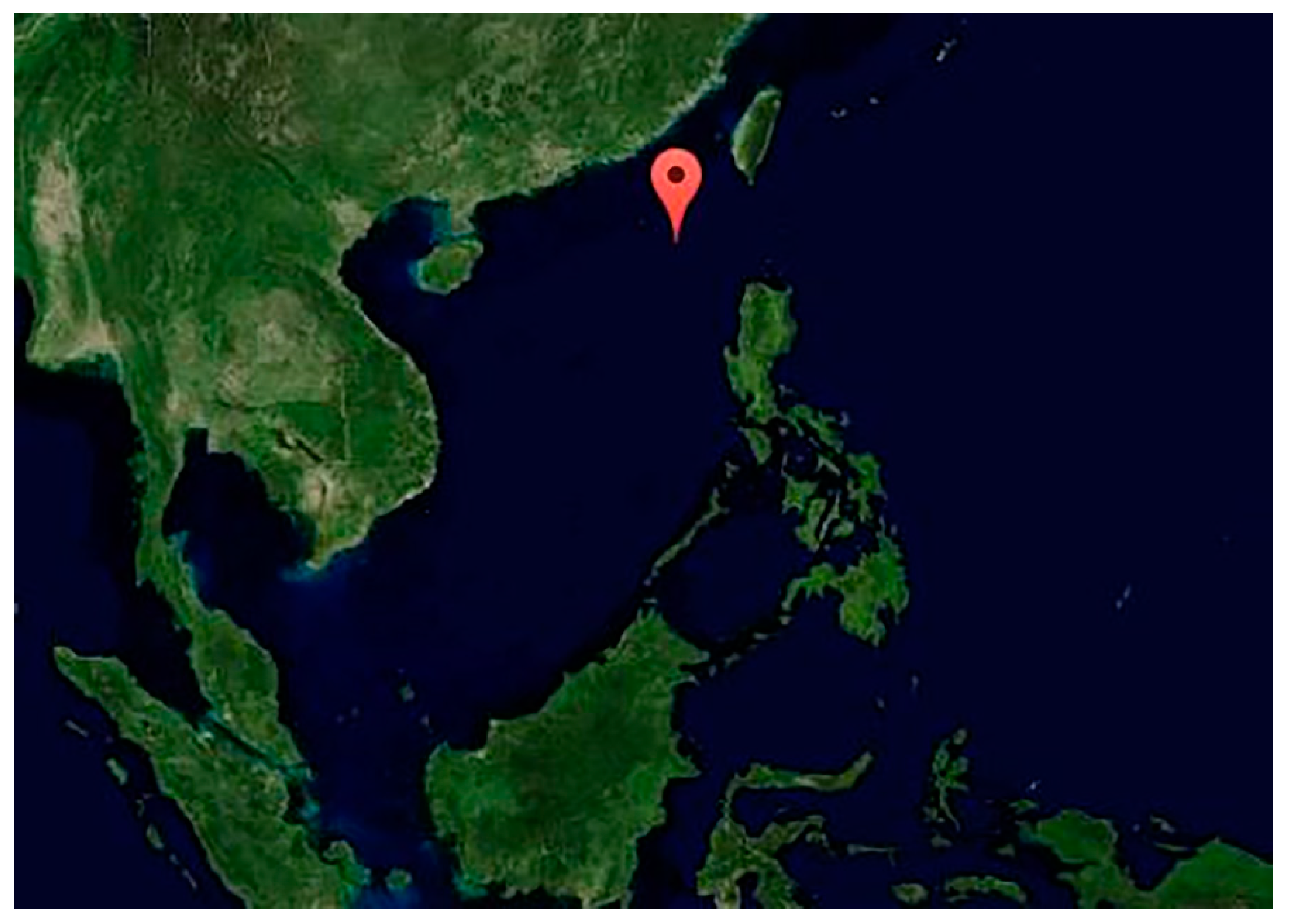
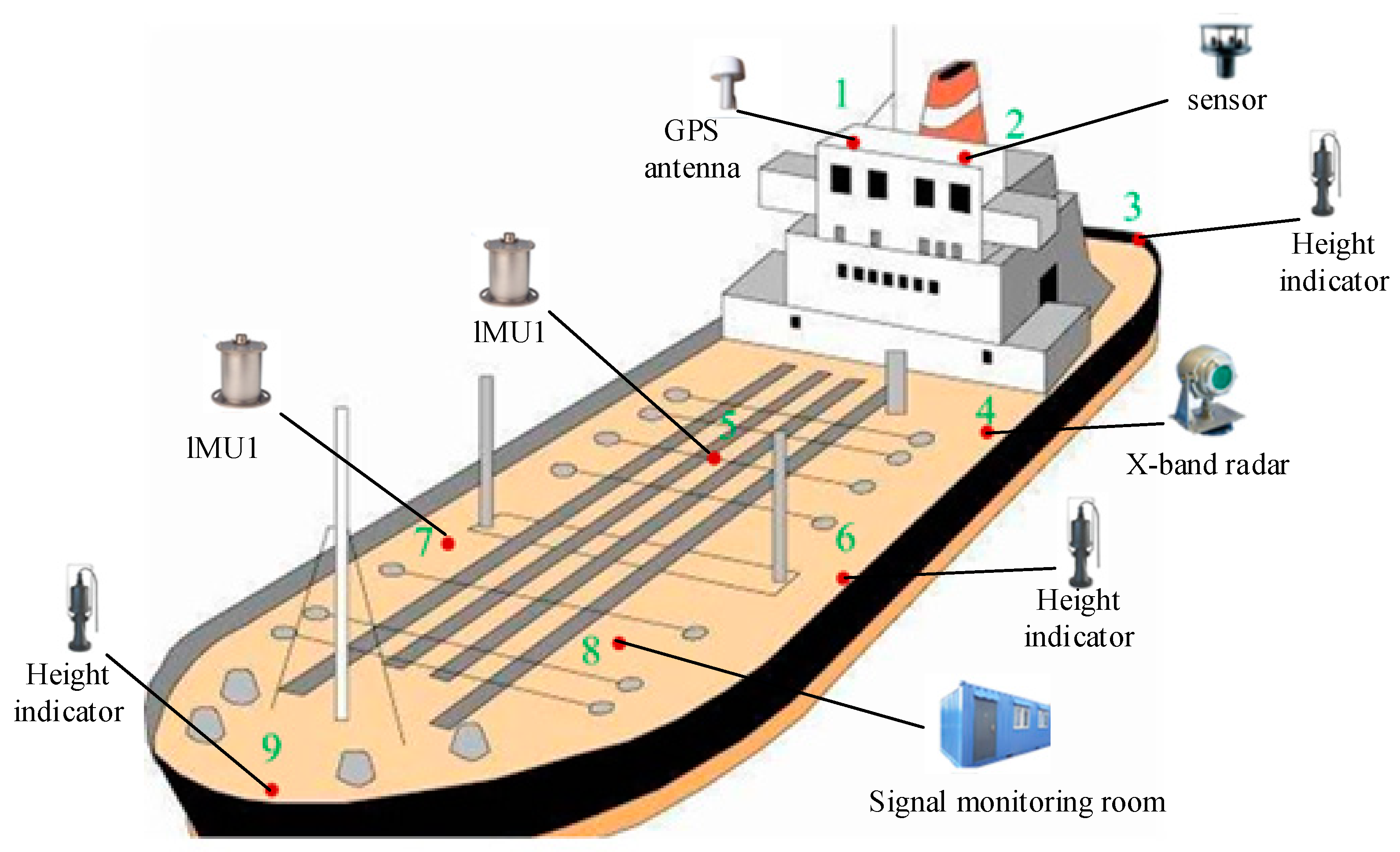
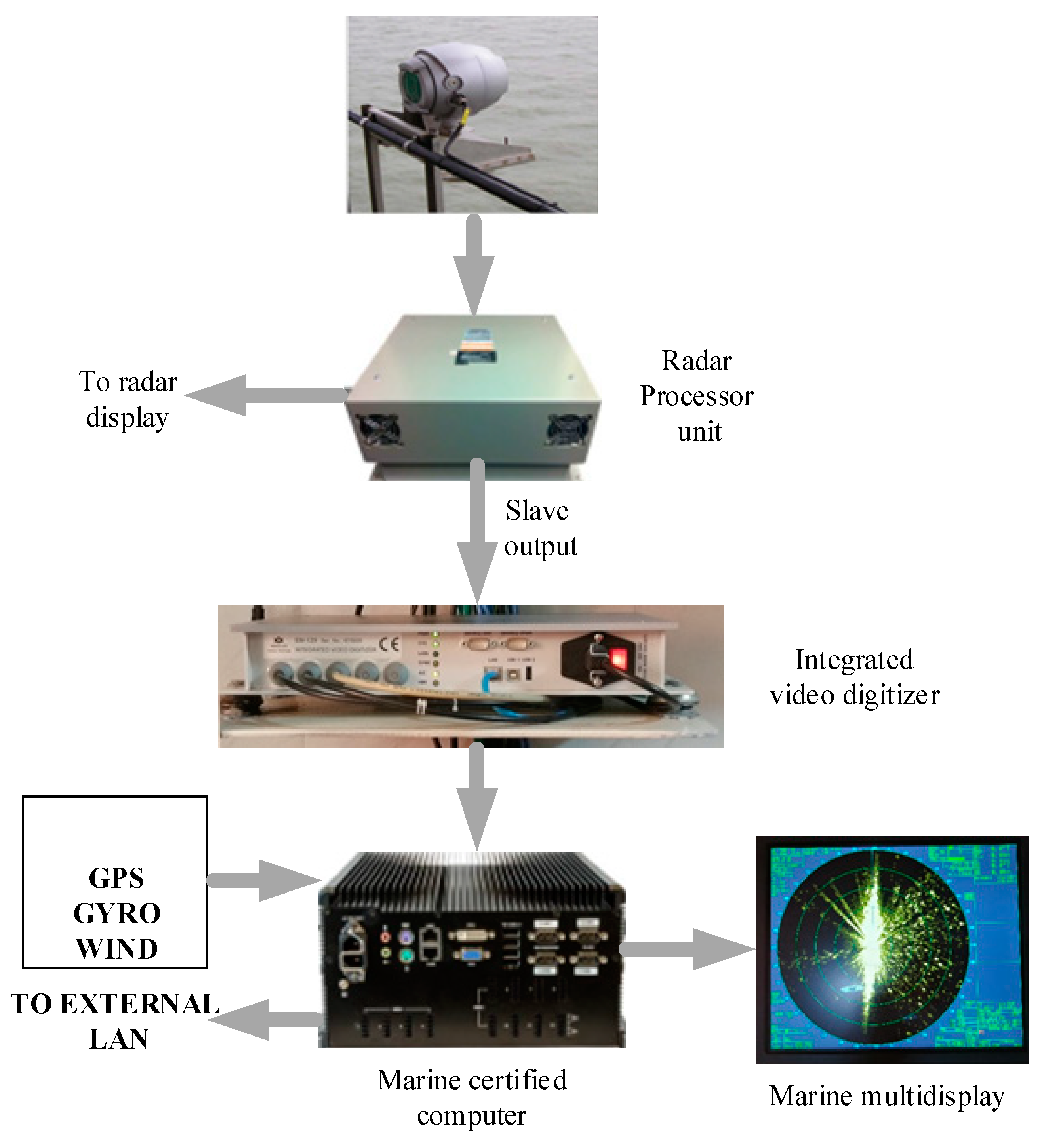
2.1. Operational Area and Monitoring System

Figure 1 shows the monitoring system that was used for the marine environmental data during PLET installation in the South China Sea (115°20′27″ E, 20°24′56″ N). During April 2019, the Offshore Oil Corporation Co. Ltd conducted a PLET sea trial. The water depth in the operational area varied from 50 m to 150 m.

A monitoring system was installed to measure the wave data to gain a better understanding of the type of marine environment that is suitable for PLET installation. The system included X-band radar, sensors, height indicators, and a Global Positioning System (GPS) antenna (Figure 2).

X-band radar was used to acquire the wave measurements in this study. The X-band radar device can be installed either on a stationary platform or moving ship. In this operation, the radar was installed on the side of the pipe-laying vessel at a height of 8 m above sea level. The X-band radar device has high temporal and spatial resolution and it consists of an appropriately sized antenna, a main unit, a control unit, and a display unit (Figure 3). After the antenna scans the ocean surface, the radar device receives echo-scattering signals from the ocean surface. These parameters were effectively estimated every few minutes by transforming signal information, such as the directional wave spectrum and the wave height. The wave information was then presented in the form of icons, a text output, and data files. This system can automatically run with a cycle time of approximately 1 min.

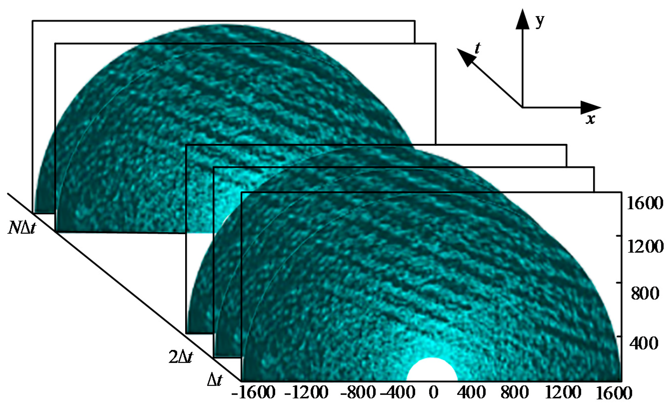
2.2. Extraction of Marine Information

The radar images of “sea clutter” are composed of backscattered echoic waves that were generated by the interaction of the radar waves with sea surface capillary waves. The surface gravity wave modulates the backscattered echoic wave, so large amounts of ocean wave information are included in the sea clutter image (Figure 4). The ocean wave data that were produced by the radar signal extraction ranged from polar coordinates to rectangular coordinates.

The sea surface can be imaged once by rotating the radar antenna. The X-band radar handles a certain number of the accumulated images in one transfer time interval. The spatial and temporal distribution function g(r, θ, t) of the gray levels was determined for 40 consecutive images per minute collected by the radar antenna (Figure 4). The antenna speed determines the time interval Δt between two consecutive images. The radius of the semicircular area was 1600 m and the radar resolution satisfied the requirements for marine environmental monitoring. The radar system performs a fast Fourier transform (FFT) on multiple g(r, θ, t) images each minute to obtain the function $I(\overrightarrow{k},\omega )$. The antenna speed of this X-band radar system was set at 15 s/rad, which meant that 40 g(r, θ, t) images could be obtained per minute, and the period of the function $I(\overrightarrow{k},\omega )$ was set at 1 min. Performing an FFT of g(r, θ, t) yielded wave number-frequency spectra that satisfied the dispersion relation for gravity waves. The dispersion relation can be expressed as:

$$\omega (\overrightarrow{k})=\sqrt{g\left|\overrightarrow{k}\right|\tanh (\left|\overrightarrow{k}\right|h)}+\overrightarrow{k}\overrightarrow{U},$$

(1)

where $\omega$ is the angular frequency, $\overrightarrow{k}=(k_r,k_{\theta })$ is the wave number vector in two directions, h is the average height of the monitoring area, and U is the surface flow velocity.

The function g(r, θ, t) was then converted while using a three-dimensional Fourier transform:

$$I(\overrightarrow{k},\omega )={\displaystyle {\int }_0^r{\displaystyle {\int }_0^{\theta }{\displaystyle {\int }_0^{T}g(r,\theta ,t_i)}}}\exp [i(k_{r}r+k_{\theta }\theta -\omega t)]drd\theta dt,$$

(2)

where $I(\overrightarrow{k},\omega )$ is the image wave number frequency spectrum, r and θ indicate the radius and the angle of the rectangular area, respectively, i is the time series, and T is the total length of the time series [22,23].

Using the dispersion relation as a band pass filter to calculate the wave number frequency interval, we eliminated the effects of the Doppler shift on the wave frequency that was measured by the radar to obtain wave number images in two dimensions:

$$\begin{array}{c}{I}^{(3)}(\overrightarrow{k})=2{\displaystyle {\int }_{\omega >0}{I}^{(2)}(\overrightarrow{k},\omega )d(\omega -\tilde{\omega })},\\ I^{(2)}(\overrightarrow{k},\omega )=\frac{{\left|I(\overrightarrow{k},\omega )\right|}^2}{ST},\end{array}$$

(3)

where S is the area of the grayscale image that reduces spectral blurring when the angle is >180°, so the part where $\omega >0$ is reserved. When the surface flow velocity is $\overrightarrow{U}$, the frequency dispersion follows Equation (1).

The ocean wave number spectrum was obtained by multiplying the modulation transfer function M and the image wave number spectrum:

$$M=k^{\beta },$$

(4)

where $\beta$ is obtained by fitting with the least squares method with $\lg k$ as the abscissa and $\lg M$ as the ordinate:

$$F^{(2)}(\overrightarrow{k})=k^{\beta }\cdot I^{(2)}(\overrightarrow{k},\omega ).$$

(5)

Furthermore, the wave direction spectrum was obtained while using the following:

$$F^{(2)}(\omega ,\theta )=\frac{k}{2\pi }\frac{\partial k}{\partial \omega }{F}^{(2)}(k,\theta ),$$

(6)

$$S(\omega )={\displaystyle {\int }_0^{2\pi }{F}^{(2)}(\omega ,\theta )}d\theta .$$

(7)

The spectra, which were measured by the radar every minute, are shown at 600 min., 3000 min., and 6000 min. in Figure 5.

3. Results of Wave Data Time Series Simulation and Spectral Estimation

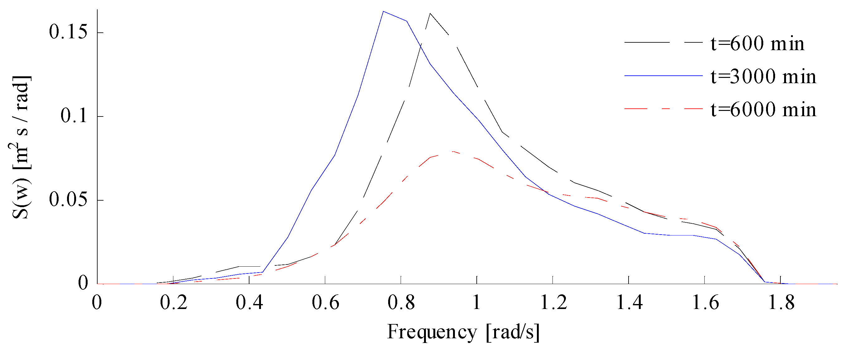
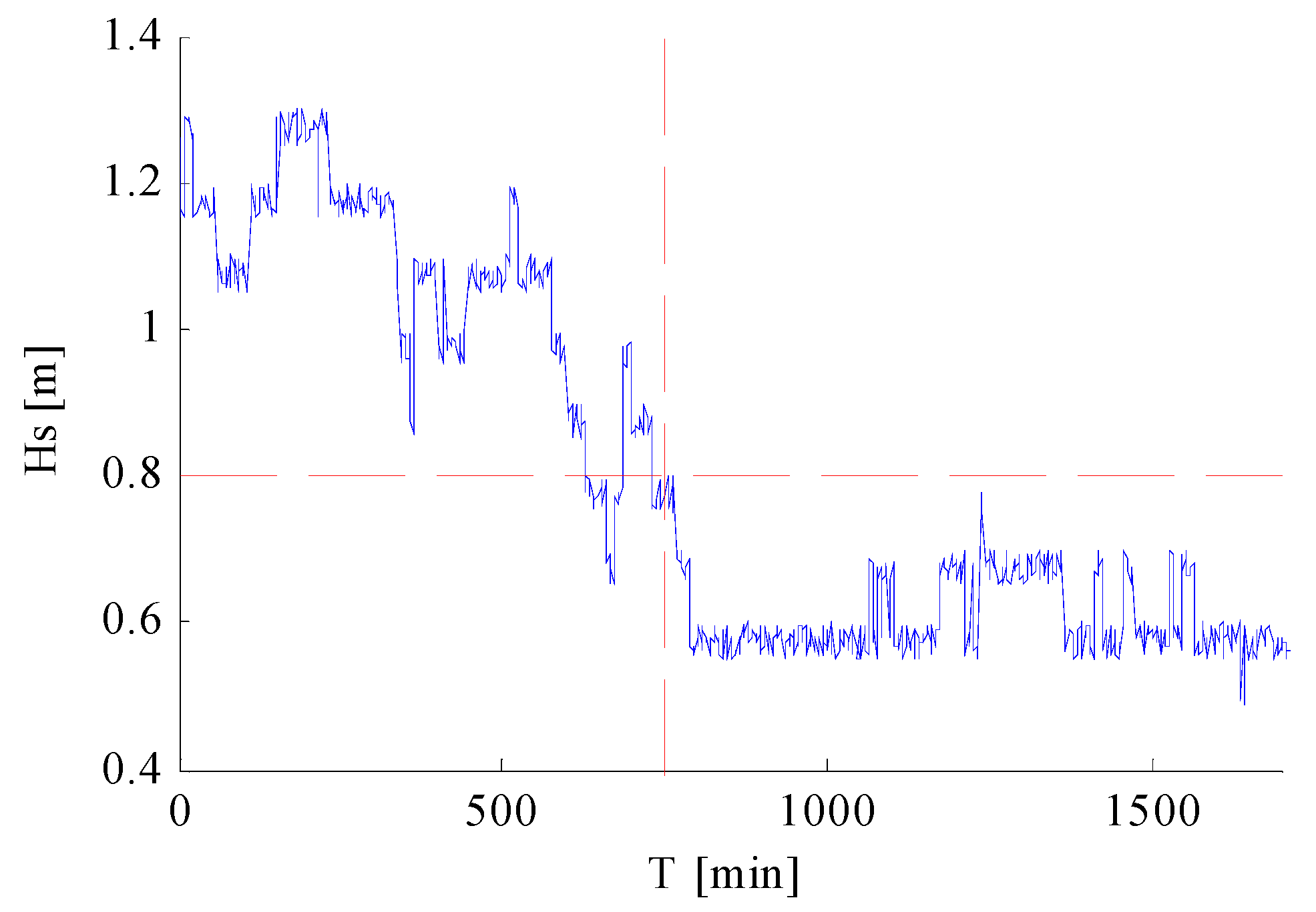
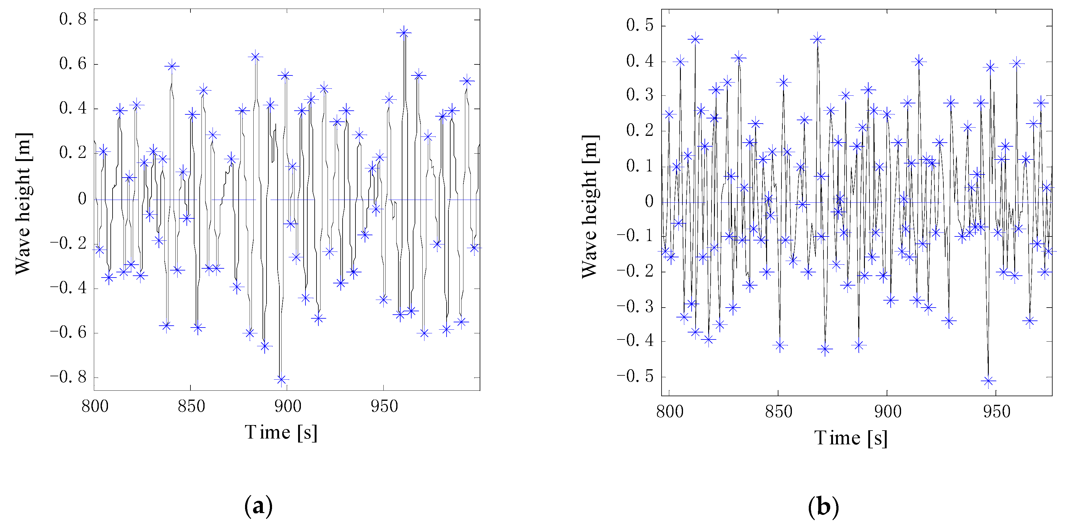
3.1. Wave Data Simulation

The wave spectra per minute obtained by the radar were simulated to obtain real-time data to represent the entire working environment, as the wave information in these wave spectra is limited and the environmental conditions during the pipe-laying operation cannot be described in detail. Using the spectrum measured by radar every minute, the significant wave height (H_s) can be calculated as:

$$H_s=4\sqrt{m_0},$$

(8)

where $m_0={\displaystyle \sum _{i=0}^N\omega \widehat{S}(\omega )}$ represents the zero-order spectral moments and the significant wave height changes over time (see Figure 6).

According to

Table 1. Classification of sea states.

Wave Scale	Wave Definition	Hs [m]
0	Calm-glassy	0
1	Calm-rippled	<0.25
2	Smooth wavelet	0.25~<0.8
3	Slight wave	0.8~<1.25
4	Moderate	1.25~<2.00

[24], the sea state during the pipe-laying operation could be divided into two scales with 750 min. as the demarcation point in the time series: smooth waves (0.25 m < H_s < 0.8 m) and slight waves (0.8 m < H_s < 1.3 m). Therefore, wave data simulation and wave spectra regression were carried out in light of these two scales.

The radar results are presented as wave spectra in terms of monitoring the area per minute. The wave spectrum over a small time interval cannot explain the distribution in the study area during the entire pipe-laying operation, so we used geometric approximation to simulate the radar wave spectra each minute to obtain real-time wave series data. The ocean wave data were then arranged in chronological order to derive the ocean history during the entire pipe-laying operation.

A useful mathematical model for such a situation is the random function (stochastic process), as denoted by X(t). The model of a stationary wave signal with a fixed spectrum S(w) is:

$$X(t)=m_0+{\displaystyle \sum _{i=1}^N\sqrt{{\widehat{s}}_i\Delta \omega }}\sqrt{2}\cos ({\omega }_{i}t+{\theta }_i),$$

(9)

where ${\theta }_i$ is the spreading direction angle, N is the total number of frequencies, i is the frequency number, $\Delta \omega$ is the sample interval for the radar in the frequency domain ${\omega }_i=i\cdot \Delta \omega$, and ${\widehat{s}}_i$ is the value of the spectrum at each frequency, which was monitored and then extracted in Section 2.2. Therefore, ${\widehat{s}}_i$ includes a certain randomness to ensure the randomness of the wave data X(t). The last integral is the zero order spectral moment m_o, and a higher order spectral moment is defined as $m_n={\displaystyle {\int }_0^{\infty }{\omega }^n\widehat{s}(\omega )}d\omega$.

Table 2. Summary of observation statistics.

Dataset	Ts [s]	T [min]	Hs [m]
Group 1	0.5	750	1.0583
Group 2	0.5	950	0.6069

gives some simple statistics for the real-time wave data transformed while using the measured spectra, including the time interval T_s, the total measurement time T, and the significant wave height H_s. To calculate the significant wave height, all of the turning points were included in the calculations.

Figure 7 shows the parts of the wave data that were acquired during the pipe-laying operation with the turning points.

3.2. Similarity Analysis of Measured and Ocean Spectra

The complete simulation wave data were used to estimate and regress the ocean spectrum during the pipe-laying operation in the South China Sea. The correlation function was used to estimate the sea spectrum.

3.2.1. Regression of the Ocean Wave Spectrum

The correlation function is a description of the stochastic process from a time domain perspective. In contrast, the spectral function describes the stochastic process from the frequency domain perspective, and both can be obtained while using a Fourier transform. The correlation and spectral functions are defined as:

$$R_{xx}(\tau )=\underset{T\to \infty }{\lim }\frac{1}{2T}{\displaystyle {\int }_{-T}^{T}x(t)x(t+\tau )}dt,$$

(10)

$$S_{xx}^{\ast }(\omega )=\underset{T\to \infty }{\lim }\frac{1}{4\pi T}{\left|X(\omega )\right|}^2,$$

(11)

where $S_{xx}^{\ast }$ is the two-sided spectral function. By applying the FFT, the correlation function and the one-sided spectrum can be expressed as:

$$\begin{array}{c}{R}_{xx}(\tau )={\displaystyle {\int }_{-\infty }^{\infty }{S}_{xx}^{\ast }(\omega )e^{i\omega \tau }}d\omega ,\\ S_{xx}(\omega )=\underset{T\to \infty }{\lim }\frac{2}{\pi }{\displaystyle {\int }_0^T{R}_{xx}(\tau )\cos \omega \tau }d\tau .\end{array}$$

(12)

The integral above was converted into a finite numerical integral that can be expressed by the sum

$$\widehat{R}(\nu \Delta t)=\frac{1}{N-\upsilon }{\displaystyle \sum _{n=1}^{N-\upsilon }x(t_n+\nu \Delta t)x(t_n)},$$

(13)

where $\tau =\nu \Delta t$, $\Delta t$ is the time interval of the wave time series data, and $\nu =0,1,2,\dots ,m(<N)$. Therefore, the corresponding numerical integration of the spectral estimation is:

$${\widehat{S}}_h=\frac{2\Delta t}{\pi }\left[\frac{1}{2}\widehat{R}(0)+{\displaystyle \sum _{\nu =1}^{m-1}\widehat{R}(\nu \Delta t)\cos \frac{\pi \nu h}{m}+\frac{1}{2}\widehat{R}(m\Delta t)\cos (h\pi )}\right],h=0,1,2,\dots ,m$$

(14)

where ${\omega }_h=h\Delta t=\frac{h\pi }{m\Delta t}$ is the frequency interval, ${\widehat{S}}_h$ is the estimated rough spectrum, and the spectral curve regressed using Equation (15) is jagged. The coarse spectra must be smoothed to improve the quality of the spectral estimation.

The Hanning weight function was adopted as a smoothing function:

$$D(\tau )=\{\begin{array}{ll}\frac{1}{2}\left(1+\cos \frac{\pi \tau }{T_m}\right),& \left|\tau \right|\le c\\ 0& \left|\tau \right|>T_m\end{array},$$

(15)

where $T_m=m\Delta t$ is the maximum value of $\tau$ in Equation (15) and is the maximum delay, and the spectral value after smoothing is expressed as:

$${\widehat{S}}_h=0.25{\widehat{S}}_{h-1}+0.5{\widehat{S}}_h+0.25{\widehat{S}}_{h+1},h=1,2,\dots ,m-1.$$

(16)

3.2.2. Theoretical Ocean Spectra

The theoretical ocean spectra were calculated while using two equations. The first is the Jonswap spectrum [25]:

$$S_{\varsigma }(\omega )=319.34\frac{H_s}{T_p^4{\omega }^5}\left\{-\frac{1948}{{(T_p\omega )}^4}\right\}{3.3}^{\exp \left[-\frac{{(0.159\omega T_p-1)}^2}{2{\sigma }^2}\right]},$$

(17)

where T_p is the peak spectral period and $\omega$ is the wave frequency, whereby

$$\sigma =\{\begin{array}{lll}0.07& \mathrm{if}& \omega <{\omega }_p\\ 0.09& \mathrm{if}& \omega \ge {\omega }_p\end{array}.$$

(18)

The second calculation uses the Ochi-Hubble double-peak spectrum and describes bimodal spectra using a superposition of two modified Pierson-Moskovitz spectra with six parameters. The spectrum includes two peaks that divide it into two parts: the swell and wind waves represent the low and high frequency parts, respectively, with each part using the three parameters H_s (significant wave height), ${\lambda }_i$ (shape parameter), and ${\omega }_p$ (wave frequency):

$$S_{\varsigma }(\omega )=\frac{1}{4}{\displaystyle \sum _{i=1}^2\frac{{(({\lambda }_i+1/4){\omega }_{p,i}^4)}^{{\lambda }_i}}{\Gamma ({\lambda }_i)}}\frac{H_{s,i}^2}{{\omega }^{4{\lambda }_i}+1}\exp \left(\frac{-({\lambda }_i+1/4){\omega }_{p,i}^4}{{\omega }^4}\right),$$

(19)

where i = 1 and 2 represent the low- and high-frequency components, respectively. The significant wave height H_s was calculated (Table 2) and it forms the foundation for the six mean parameters in Equation (20).

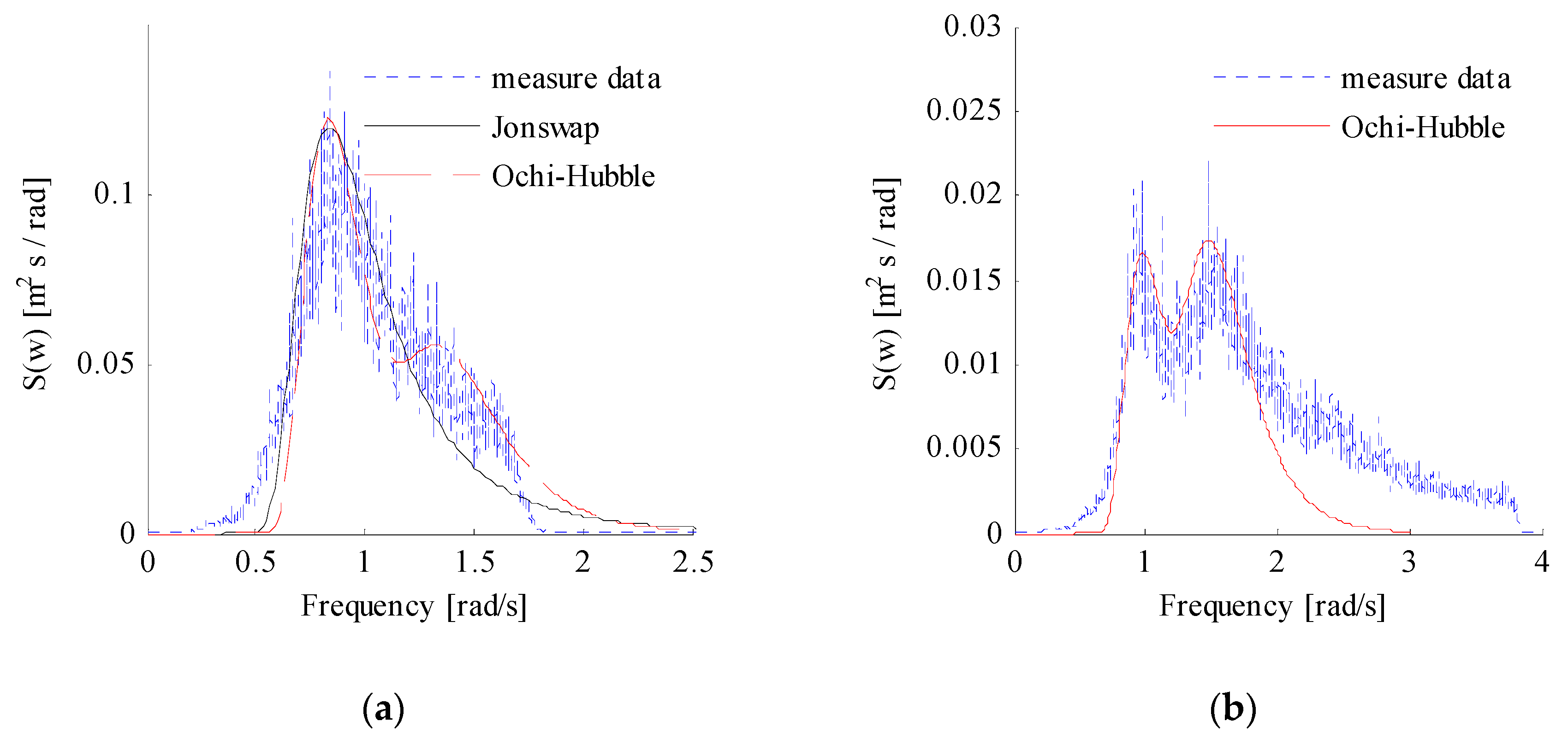
3.2.3. Comparison and Analysis of the Measured and Ocean Spectra

The measured spectra were regressed while using a correlation function, and the theoretical spectra at the same sea level were also calculated. The value of the smooth function was set as 2000 to retain the original shape and reduce the total wave energy loss. On the basis of the regressed spectra, only theoretical spectra with similar shapes were calculated (Figure 8, where the dotted lines represent the regressed spectra).

The regressed spectrum was similar to the Ochi-Hubble spectrum when H_s = 1.0583 m (Figure 8a), although the valley in the middle of two peaks of the regressed spectrum is a deviation from the theoretical spectrum. The Jonswap spectrum ignored the peak energy of the wind waves. The regressed spectrum was a double-peak spectrum of the sea state that represented the dominance of the swell.

Another spectrum showed a double peak with approximately the same height, which means that the wave energies of the low- and high-frequency parts were nearly equal; therefore, only the Ochi-Hubble theoretical spectrum was calculated during the similarity analysis. The low-frequency part represents the swell component of a wave, while the high-frequency part indicates a wind wave. According to a regressed spectrum with H_s = 0.6069 m, the mixed wind waves and swell have comparable energies. From a sea state, with H_s = 1.0583 m, to a slightly lower sea condition of H_s = 0.6069 m, the sea state varied from swell-dominated to mixed wind wave and swell throughout the PLET installation.

The peak frequency of the measured spectrum with H_s = 1.0583 m was similar to the first peak frequency of another spectrum, with H_s = 0.6069 m, which means that the period of the swell remained approximately the same during the PLET operations. The measured spectra were more similar to the theoretical spectra at low frequencies and at the high-frequency peak (Figure 8b). The other remaining high-frequency regions deviated from the theoretical spectra because of the energy dissipation of a lower sea state. This indicates that the double-peak Ochi-Hubble spectrum can be used to analyze and forecast the marine environment during PLET operations in the South China Sea.

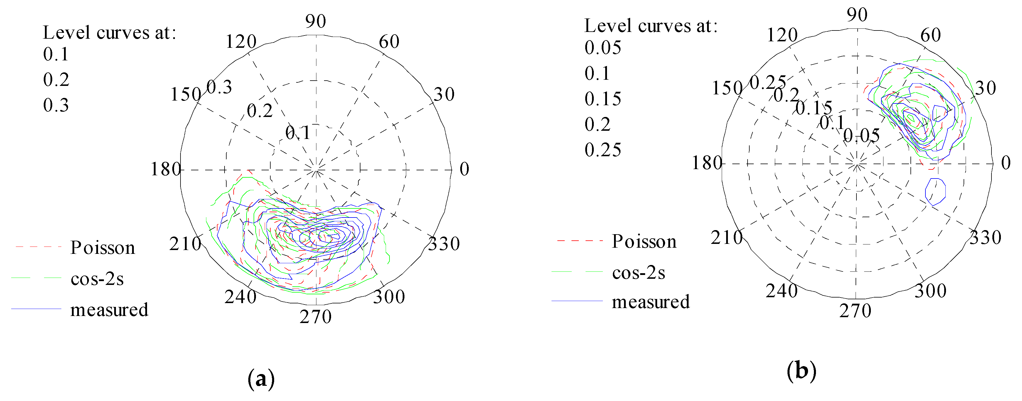
3.3. Direction Spectrum Regression and Spreading Function Analysis

The direction wave spectrum is a plot that shows the distribution of the energy with the wave period and direction. Using the direction spectrum, the original directions of the waves and their periods can be determined. The spectrum consists of single or multiple wave systems and separate wind wave and swell systems. The direction spectrum can be calculated as:

$$S_d=S(\omega )\cdot D(\omega ,\theta ),$$

(20)

where $S(\omega )$ is the frequency spectrum, $D(\omega ,\theta )$ is the direction spreading function, f is the frequency, and $\theta$ is the direction. There are two common families of direction-spreading functions: the cos₋2s distribution that was introduced by Longuet-Higgins and the Poisson distribution derived by Lygre and Krogstad [26].

Table 3. Theoretical direction spreading functions.

Function	Expression	Parameter Range	Fourie Coefficient
cos-2s	$\frac{1}{2\pi }\frac{\Gamma (s+1)}{\sqrt{\pi }\Gamma (s+1/2)}{\cos }^{2s}\left(\frac{\theta }{2}\right)$	0 < s	$\frac{{\Gamma }^2(s+1)}{\Gamma (s+n+1)\Gamma (s-n+1)}$
Poisson	$\frac{1}{2\pi }\left[1+2{\displaystyle {\sum }_{n=1}^{\infty }{x}^{n^2}}\cos (n\theta )\right]$	0 < x < 1	$x^{n^2}$

lists the formulae and parameters of these two spreading functions.

In this study, the direction spectrum that was measured using radar was compared with the direction spectrum calculated from the theoretical direction spreading via Equation (20) to determine which of the spreading functions satisfied the conditions in the operational area. Spectra were regressed using the real-time wave data.

Figure 9 shows the measured direction spectrum and the calculated spectrum with H_s = 1.0583 m and H_s = 0.6069 m, respectively. There are two closed contours within the innermost level of the measured spectrum (Figure 9a). This means that the wave energy component decreased to approximately 240° after the wind direction shifted by approximately 45° to the east. The contours are the densest at approximately 285° along the main wave direction relative to the current wind direction. As shown in Figure 9a, the outline of the measured direction spectrum was similar to that calculated from the Poisson spreading function; the inconsistent upper left shape was a result of shifting wind direction and energy.

The calculated direction of the Poisson function is still more similar to the measured value than that calculated while using the cos-2s function (Figure 9b). In addition to the intensive contour, another contour indicates the swell from approximately 140°, which was also consistent with the two-dimensional spectra. This shows that the swell and wind waves coexisted during this monitoring procedure. The wind wave information did not show any changes in the wind direction, and the outline of the measured spectrum matched the spectrum of the Poisson spreading function better than that shown in Figure 9a.

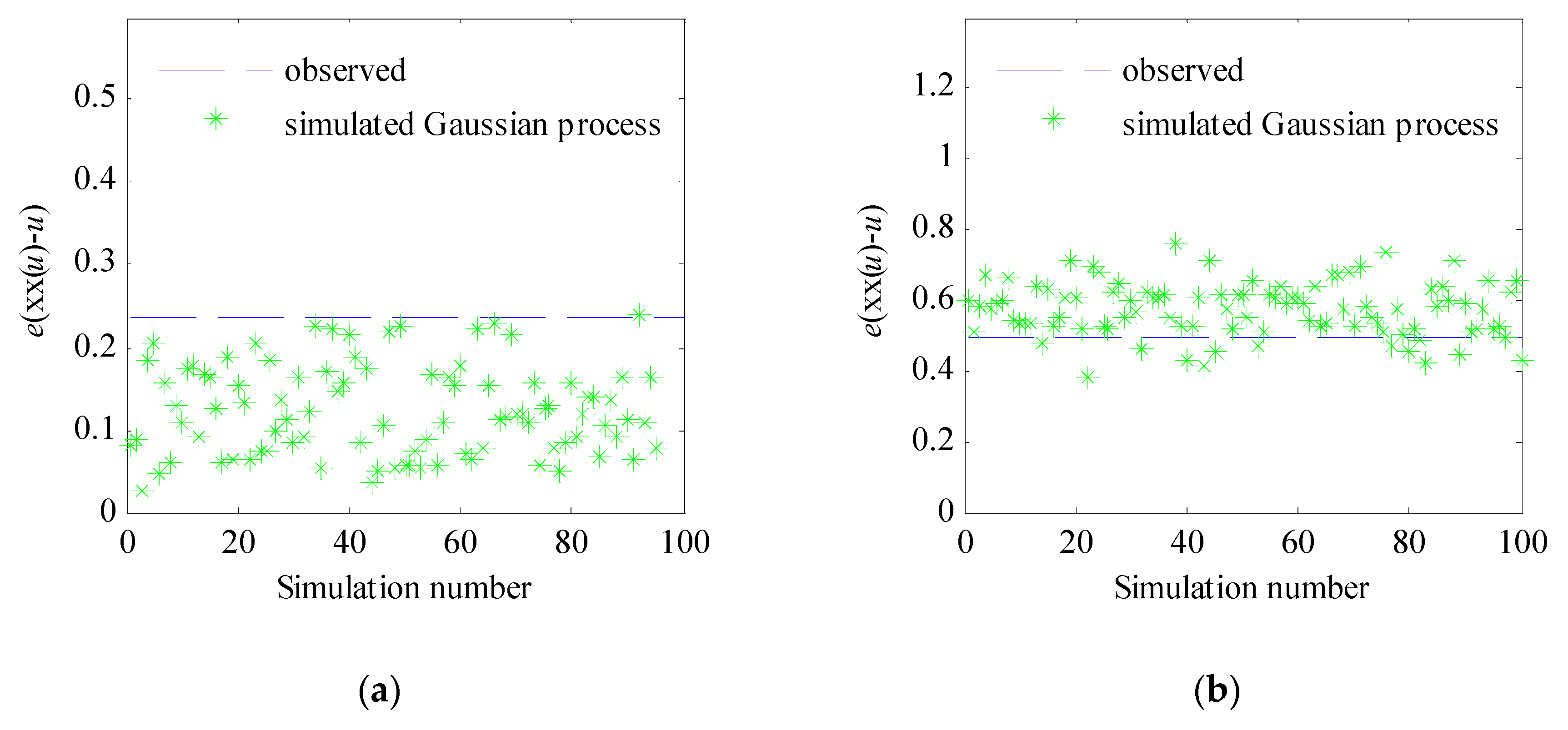
3.4. Gaussian Processing Test

A sea state under stationary conditions, model X(t), was assumed to be similar to a Gaussian process, which is a stationary and ergodic stochastic process with an average value of zero. Real wave data seldom perfectly support Gaussian assumptions. The Gaussian case is well modeled, and there are approximate methods to calculate the wave characteristics from a Gaussian spectrum. Gaussian fitting was conducted on the wave data calculated from the radar-obtained spectrum to determine the degree of departure from a Gaussian process [27].

The function e(g) was used to calculate how much the data departed from a Gaussian process. The definition of e(g) is:

$$\begin{array}{c}e(g)={\left({{\displaystyle {\int }_{-\infty }^{\infty }(g(u)-u)}}^{2}du\right)}^{1/2},\\ g(u)=\{\begin{array}{l}\sqrt{-2\ln (2\mathsf{\pi }\stackrel{⌢}{V}(\sigma u+m))}\\ -\sqrt{-2\ln (2\mathsf{\pi }\stackrel{⌢}{V}(\sigma u+m))}\end{array},\end{array}$$

(21)

where $V(u)$ is the crossing-density function, which yields the average number per unit time or space of up-crossings of level u. The basic definition of the crossing function is $V(u)=E[\mathrm{numbers} \mathrm{of} \mathrm{up}\text{-}\mathrm{crossing} \mathrm{of} \mathrm{level} u \mathrm{by} X(t)]$, where E is the expected value and V is approximated as:

$$V(u)=\frac{1}{T}{\displaystyle \sum _i{l}_{(m_i,M_i]}}(u)=\widehat{V}(u),$$

(22)

where $l_{(m_i,M_i]}(u)=1$ if minimum < u < maximum and 0 otherwise. The minimum and maximum are the local wave extremes of the index and u is a variable of the different levels of the crossing-density function and the transformed function produced by the empirical up-crossing density that was observed at time T.

100 group Gaussian processes were simulated to calculate the degree of departure from a Gaussian fit while using the spectrum that was regressed from the observed data. Figure 10 shows the relationship between the simulation model and the degree of deviation, e(g). Few simulated Gaussian models exceeded the e(g) value of 0.273 for the observed data at H_s = 1.0583 m, so this process slightly deviated from Gaussian behavior (Figure 10a). However, most of the simulated data exceeded the e(g) value of 0.495 for H_s = 0.6069 m, which means that this process was more similar to a Gaussian process (Figure 10b).

4. Discussion

The wave processes that were measured during the pipe-laying operation were similar to a Gaussian process, but there was a departure from this when H_s was 1.0609 m. This begs the question of whether the probability distribution of the wave parameters also satisfied the Gaussian probability distribution or another distribution. Because of this question, we calculated the wave parameter probability distribution of the measured data to compare it with the theoretical distribution.

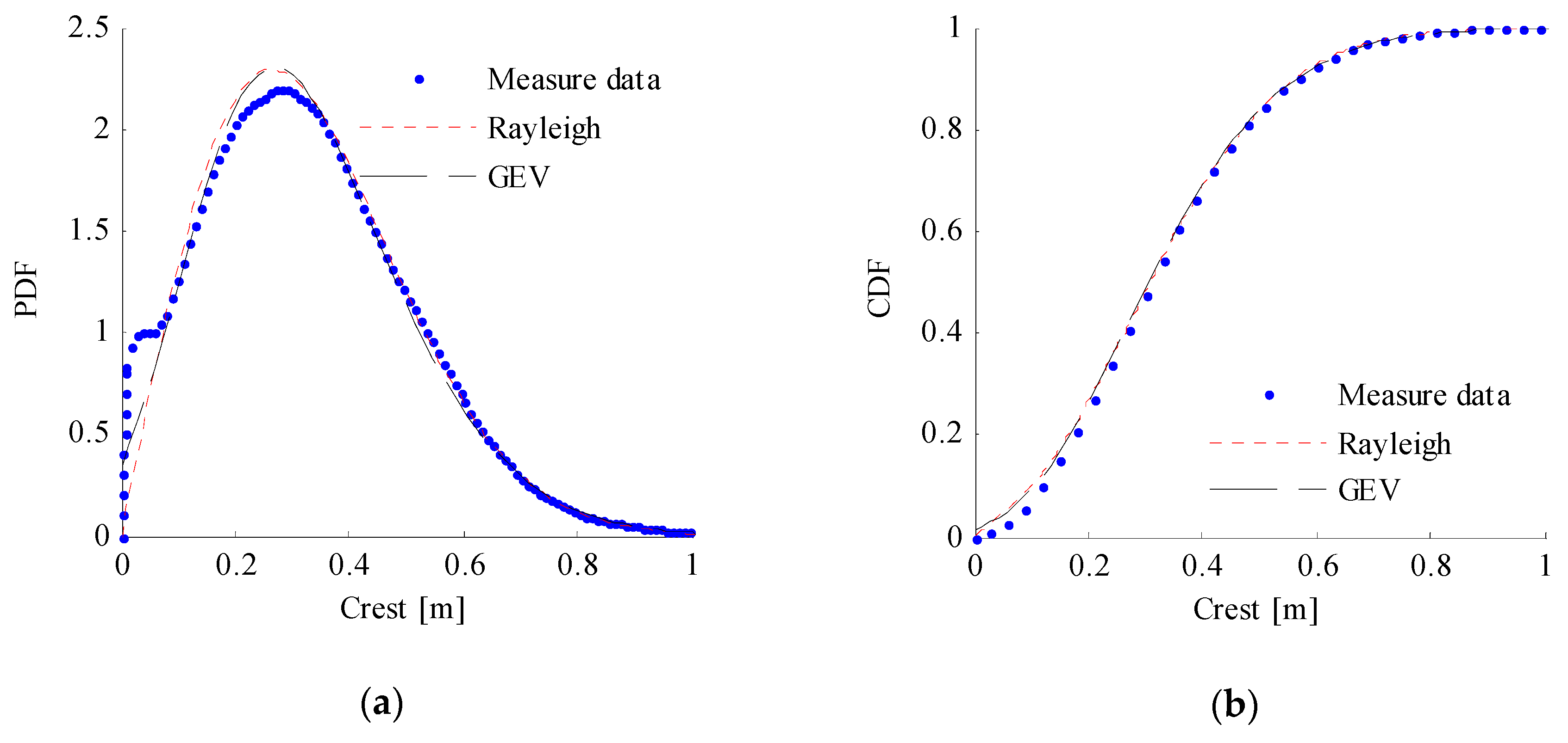
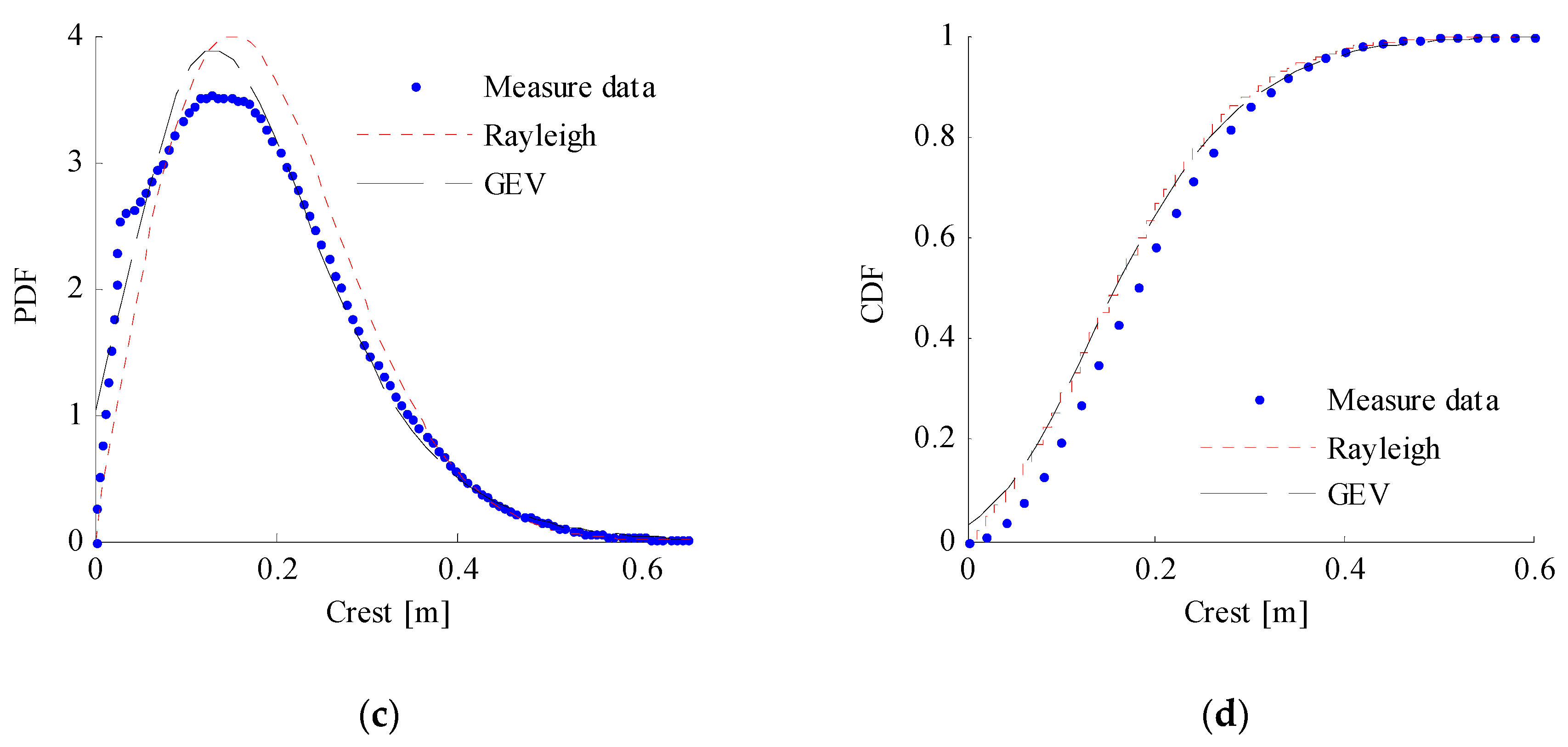
4.1. Theoretical Approximations of Wave Distribution

Forecasting the wave parameters requires obtaining the distribution of the wave characteristics. To select the most suitable distribution, we calculated the Rayleigh and generalized extreme value (GEV) distributions and the Longuet-Higgins joint distribution to describe the marginal and joint parameters.

The most frequently used model for a Gaussian sea is the Rayleigh distribution. In a Gaussian sea, the Rayleigh approximation works very well for high waves. The standardized Rayleigh variable R has a density given by $f(r)=r\exp (-r^2/2)$. In fact, this is a conservative approximation, because the probability is

$$\mathrm{P}(A>b)\le \mathrm{P}(R>4\ast b/Hs)=e^{-8b^2/H{s}^2},$$

(23)

so the approximation becomes more accurate as level b increases.

In wave analysis, the specific focus is to find extreme quantities and calculate significant values for a wave series. These values are often used to predict how large the extreme values might become outside the observed data when the number of observations is limited. Weibull and Gumbel analyses, which are two extreme value distributions, are commonly used to perform this type of analysis. Both of these analyses are part of the GEV family of extreme value distributions. The GEV distribution has the following distribution function:

$$F(x;k,\mu ,\sigma )=\{\begin{array}{ll}\exp \left\{-{(1-k(x-\mu )/\sigma )}^{1/k}\right\},& if k\ne 0,\\ \exp \left\{-\exp \left\{-(x-\mu )/\sigma \right\}\right\},& if k=0,\end{array}.$$

(24)

For k(x – µ) < σ, σ > 0, and k and µ are arbitrary. The case k = 0 is the limit when $k\to 0$ for both distributions.

In addition to the marginal distribution, the joint distribution of the wave parameters must also be analyzed. The Longuet-Higgins model provides approximate distributions by considering the joint distribution of the envelope amplitude and the time derivative of the envelope phase [28]. This approach seemed to give relatively accurate results for waves with significant amplitudes. In addition to the significant height H_s and the peak period, the Longuet-Higgins density depends on the spectral width parameter $\nu$. The density function is then:

$$f_{T,A}(t,x)=C_{LH}{\left(\frac{x}{t}\right)}^2\exp \left\{-\frac{x^2}{8}[1+{\nu }^{-2}{(1-t^{-1})}^2]\right\},$$

(25)

where the parameter $\nu =\frac{m_0{m}_2}{m_1^2}-1$ and $C_{LH}=\frac{1}{8}{(2\pi )}^{-1/2}{\nu }^{-1}{[1+{(1+{\nu }^2)}^{-1/2}]}^{-1}$.

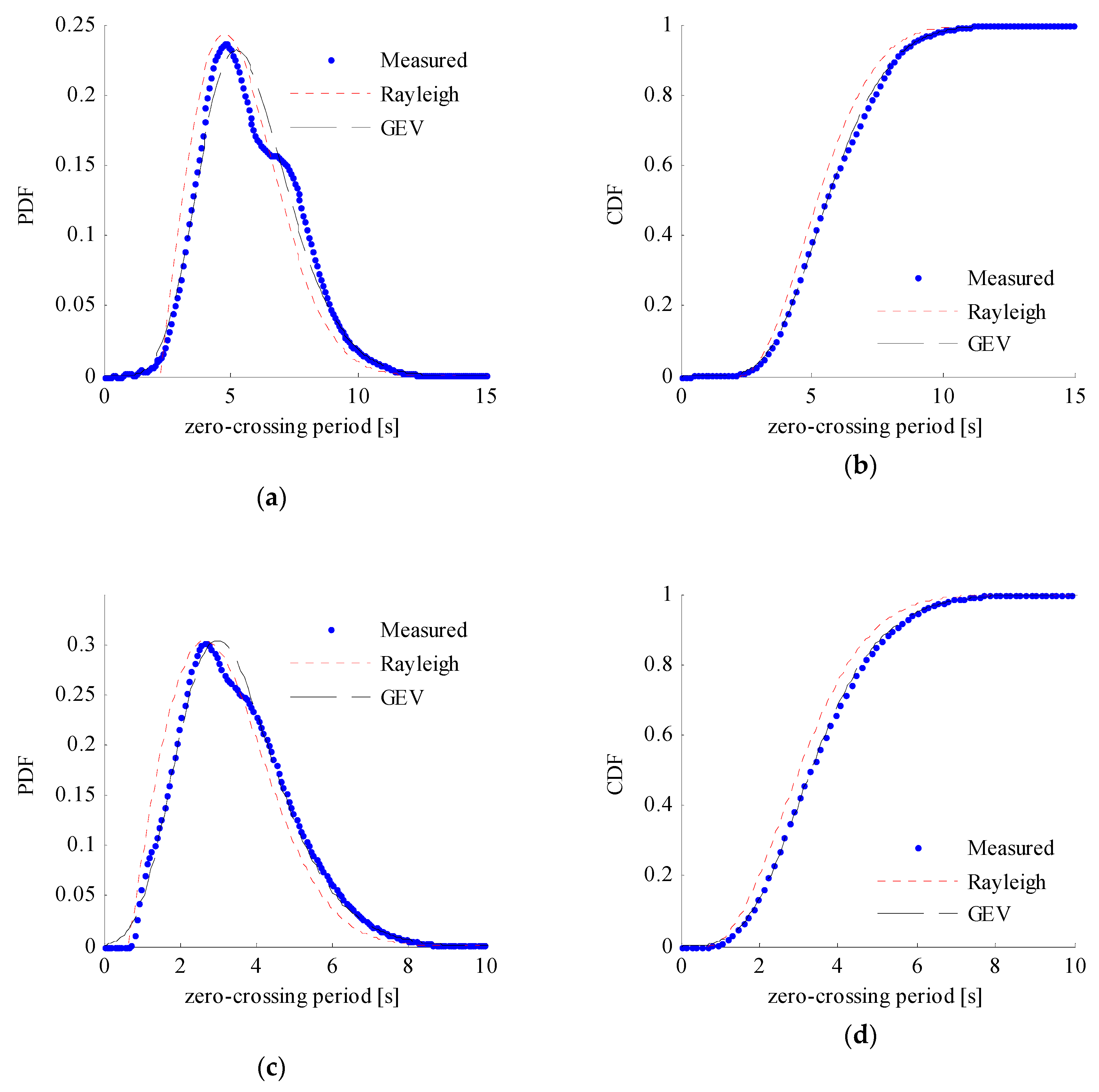
4.2. Marginal Distribution of Wave Characteristics

This section focuses on analysis of the marginal distribution of the wave characteristics. The density values of the wave crests, troughs, and zero-crossing period T calculated while using the Rayleigh and GEV distributions were compared with the empirical distribution that was estimated from the complete observed dataset. The probability density function (PDF) and cumulative distribution function (CDF) were then calculated.

Figure 11 and Figure 12 show that the cumulative distribution and the probability density of the GEV distributions for the crest and trough heights were closer to the measured data, which shows that these are the most suitable distributions for the wave crest and the trough height during operation.

When compared with the results for H_s = 0.6069 m, the Rayleigh distribution was also similar to the measured data, which means that the Rayleigh distribution can also be used to predict wave parameter distribution for relatively high sea states. The crest and trough distributions showed similar trends and the same axis range because these two sea conditions were lower during PLET operation when compared with the other sea state parameters.

The cumulative distribution of the GEV zero-crossing period was more similar to the measured data than the Rayleigh distribution (Figure 13). For the probability density of the zero-crossing period, the GEV distribution was more consistent with the measured data, with the exception of the peak values. When the wave extremes and the zero-crossing period are included, the GEV distribution can give suitable marginal distributions of the wave parameters.

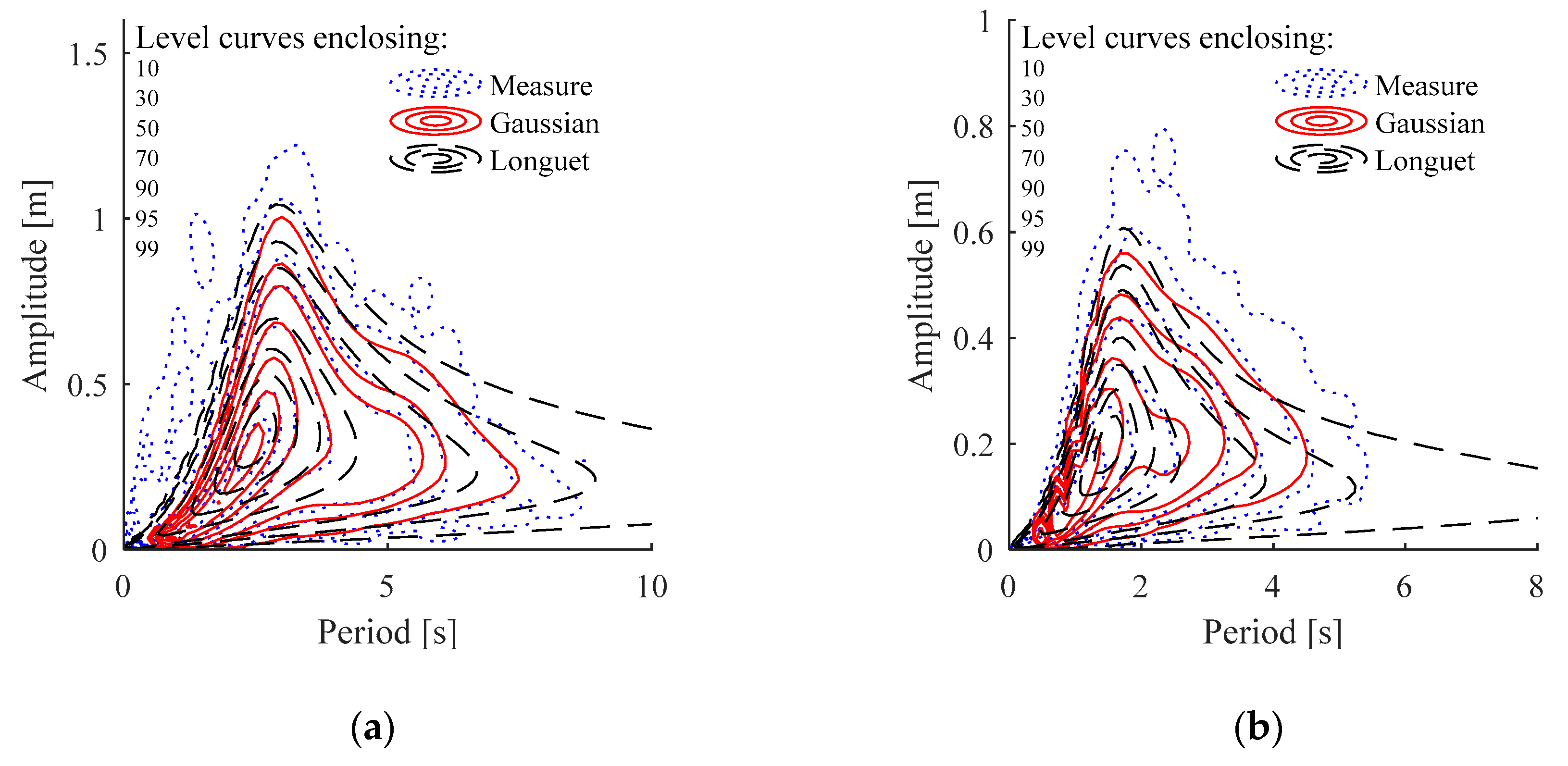
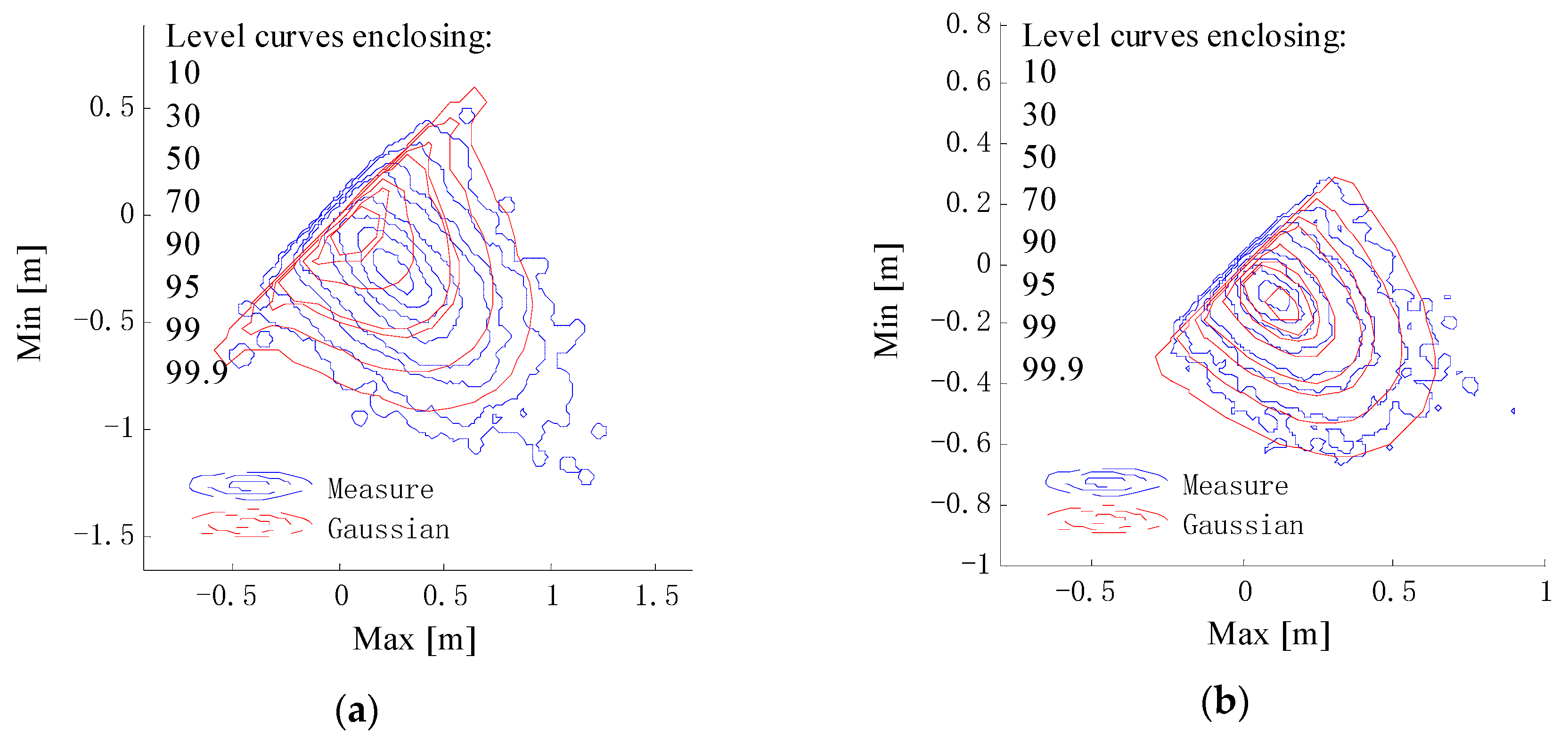
4.3. Joint Density of Wave Characteristics

An analysis of the joint density of the typical wave characteristics provides more reliable statistical estimates of the densities. We calculated the joint densities of the amplitude and the period, as well as the maximum and subsequent minimum.

From the resulting joint distribution of the amplitude and the corresponding period (Figure 14), the Gaussian model produced a distribution that was more similar to that of the measured data when compared with the Longuet-Higgins model. This may occur because the Longuet-Higgins model is used to calculate relatively accurate estimates of large waves. While the extreme values that were calculated using the Gaussian process were smaller than the measured values, the Gaussian method also satisfactorily forecast the wave characteristics. However, if the Gaussian model is used to predict the amplitude and the corresponding period, it can underestimate the wave data when compared with the real environmental data.

The Longuet-Higgins model was only used for the amplitude and period, so only the Gaussian model was used for the joint distribution of the maximum and corresponding local minimum. The maximum and minimum values showed the same symmetrical distribution as the crest and trough did, thereby also satisfying the Gaussian assumptions. The Gaussian model can give a very close distribution for the maxima and minima, especially for the sea state H_s = 0.6069 m (Figure 15). The similarity between the Gaussian model and measured data decreased with increasing H_s, thereby resembling the results for the joint distribution of the amplitude and period.

5. Conclusions

We have presented a system for monitoring the marine environment during PLET installation and used it to monitor the waves in real time and obtain images of sea clutter in the South China Sea. This study focused on measurement and analysis of the wave motion throughout the entire PLRT operation. The frequency spectra were regressed and investigated via Jonswap and double-peak Ochi-Hubble similarity analyses. The regressed spectra of two sea states were both highly similar to a double-peak spectrum, which indicated that the Ochi-Hubble spectrum was preferable for forecasting marine environments for offshore operations. The direction spectrum that was calculated from a Poisson spreading function was the most suitable for depicting the wave spreading direction of the area studied during operation. These two sea states were separated on the basis of their H_s values, which showed that H_s = 0.6069 m was more similar to a Gaussian process, but higher H_s values slightly deviated from Gaussian behavior. For the marginal distribution of wave characteristics, such as the crest, trough height, and zero-crossing period, the GEV distribution provided the most relevant results for both the probability density and cumulative density distributions. The Gaussian model provided a relatively accurate estimate of the joint distribution of the amplitude and period along with the maximum and minimum. The empirical joint distribution of the measured data with H_s = 1.0583 m slightly deviated from the Gaussian results, which indicated that the Gaussian model may give lower predictions for the wave parameters in high sea states. The wave monitoring data available during PLET installation for predicting wave transformation are limited, but it can provide context for future pipe-laying testing and process improvement. The data recorded that were using the field monitoring system are invaluable and can be referenced for the design and analysis of future projects.

References

1. Bruschi, R.; Vitali, L.; Marchionni, L.; Parrella, A.; Mancini, A. Pipe technology and installation equipment for frontier deep water projects. Ocean Eng. 2015, 108, 369–392. [Google Scholar] [CrossRef]
2. Hosseinlou, F.; Mojtahedi, A. Developing a robust simplified method for structural integrity monitoring of offshore jacket-type platform using recorded dynamic responses. Appl. Ocean Res. 2016, 56, 107–118. [Google Scholar] [CrossRef]
3. Zhang, Q.; Draper, S.; Cheng, L.; An, H. Scour below a subsea pipeline in time varying flow conditions. Appl. Ocean Res. 2016, 55, 151–162. [Google Scholar] [CrossRef] [Green Version]
4. Sollund, H.A.; Vedeld, K.; Fyrileiv, O.; Hellesland, J. Improved assessments of wave-induced fatigue for free spanning pipelines. Appl. Ocean Res. 2016, 61, 130–147. [Google Scholar] [CrossRef]
5. Nielsen, U.D.; Stredulinsky, D.C. Sea state estimation from an advancing ship–A comparative study using sea trial data. Appl. Ocean Res. 2012, 34, 44. [Google Scholar] [CrossRef]
6. Wang, F.; Chen, J.; Gao, S.; Tang, K.; Meng, X. Development and sea trial of real-time offshore pipeline installation monitoring system. Ocean Eng. 2017, 146, 468–476. [Google Scholar] [CrossRef]
7. Tian, X.; Wang, P.; Li, X.; Wu, X.; Lu, W.; Wu, C.; Hu, Z.; Rong, H.; Sun, H.; Wang, A.; et al. Design and application of a monitoring system for the floatover installation. Ocean Eng. 2018, 150, 194–208. [Google Scholar] [CrossRef]
8. Rachmayani, R.; Ningsih, N.S.; Adiprabowo, S.R.; Nurfitri, S. Ocean wave characteristic in the Sunda Strait using Wave Spectrum Model. IOP Conf. Ser. Earth Environ. Sci. 2018, 139, 012025. [Google Scholar] [CrossRef] [Green Version]
9. Hui, X.; Miao, M.; Yan, L. Analysis of the Measured Wave Data around Toumen Island Sea Area in Taizhou. In Proceedings of the 2015 International Conference on Intelligent Transportation, Big Data and Smart City, Halong Bay, Vietnam, 19–20 December 2015; pp. 113–116. [Google Scholar] [CrossRef]
10. Venkatesan, R.; Vengatesan, G.; Vedachalam, N.; Muthiah, M.A.; Lavanya, R.; Atmanand, M.A. Reliability assessment and integrity management of data buoy instruments used for monitoring the Indian Seas. Appl. Ocean Res. 2016, 54, 1–11. [Google Scholar] [CrossRef]
11. Sun, S.Z.; Li, H.; Sun, H. Measurement and analysis of coastal waves along the north sea area of China. Pol. Marit. Res. 2016, 23, 72–78. [Google Scholar] [CrossRef]
12. O’Reilly, W.C.; Olfe, C.B.; Thomas, J.; Seymour, R.J.; Guza, R.T. The California coastal wave monitoring and prediction system. Coast. Eng. 2016, 116, 118–132. [Google Scholar] [CrossRef] [Green Version]
13. Kim, B.N.; Choi, B.K.; Kim, S.H.; Kim, D.S. Real-time wave height measurements using a cable type wave monitoring system in shallow waters. In Proceedings of the 2015 IEEE/OES Eleveth Current, Waves and Turbulence Measurement (CWTM), St. Petersburg, FL, USA, 2–6 March 2015. [Google Scholar]
14. Ruju, A.; Passarella, M.; Trogu, D.; Buosi, C.; Ibba, A.; De Muro, S. An Operational Wave System within the Monitoring Program of a Mediterranean Beach. J. Mar. Sci. Eng. 2019, 7, 32. [Google Scholar] [CrossRef]
15. Seim, H.E.; Fletcher, M.; Mooers, C.N.K.; Nelson, J.R.; Weisberg, R.H. Towards a regional coastal ocean observing system: An initial design for the Southeast Coastal Ocean Observing Regional Association. J. Mar. Syst. 2009, 77, 261–277. [Google Scholar] [CrossRef]
16. Singh, U.N.; Nicolae, D.N.; Mori, Y.; Shimada, S.; Shiina, T.; Baji, H.; Takemoto, S. Dynamic analysis of sea wave data measured by LED lidar. In Proceedings of the SPIE Remote Sensing, Edinburgh, UK, 26–29 September 2016; Volume 10006, p. 100060G. [Google Scholar] [CrossRef]
17. Seemann, J.; Carrasco, R.; Stresser, M.; Horstmann, J.; Stole-Hentschel, S.; Trulsen, K.; Borge, J.C.N. An Operational Wave Monitoring System Based on a Dopplerized Marine Radar. In Proceedings of the OCEANS 2017-Aberdeen, Aberdeen, UK, 19–22 June 2017. [Google Scholar]
18. Al-Hajeri, S.; Wylie, S.R.; Shaw, A.; Al-Shamma’a, A.I. Real time EM waves monitoring system for oil industry three phase flow measurement. J. Phys. Conf. Ser. 2009, 178, 012030. [Google Scholar] [CrossRef]
19. Yasui, T.; Nakamura, R.; Kawamoto, K.; Ihara, A.; Fujimoto, Y.; Yokoyama, S.; Inaba, H.; Minoshima, K.; Nagatsuma, T.; Araki, T. Real-time monitoring of continuous-wave terahertz radiation using a fiber-based, terahertz-comb-referenced spectrum analyzer. Opt. Express 2009, 17, 17034–17043. [Google Scholar] [CrossRef] [PubMed] [Green Version]
20. Li, H.; Terada, H.; Yamada, A. Real-time monitoring system of vortex wind field using coded acoustic wave signals between parallel array elements. Jpn. J. Appl. Phys. 2014, 53, 7–18. [Google Scholar] [CrossRef]
21. Armenio, E.; Ben Meftah, M.; Bruno, M.F.; De Padova, D.; De Pascalis, F.; De Serio, F.; Di Bernardino, A.; Mossa, M.; Leuzzi, G.; Monti, P. Semi enclosed basin monitoring and analysis of meteo, wave, tide and current data: Sea monitoring. In Proceedings of the 2016 IEEE Workshop on Environmental, Energy, and Structural Monitoring Systems (EESMS), Bari, Italy, 13–14 June 2016; pp. 1–6. [Google Scholar] [CrossRef]
22. Young, I.R.; Rosenthal, W.; Ziemer, F. A three-dimensional analysis of marine radar images for the determination of ocean wave directionality and surface currents. J. Geophys. Res. Oceans 1985, 90, 1049–1059. [Google Scholar] [CrossRef] [Green Version]
23. Senet, C.M.; Seemann, J.; Flampouris, S.; Ziemer, F. Determination of bathymetric and current maps by the method DiSC based on the analysis of nautical X-band radar image sequences of the sea surface. IEEE Trans. Geosci. Remote Sens. 2008, 46, 2267–2279. [Google Scholar] [CrossRef]
24. Young, I.R. Global ocean wave statistics obtained from satellite observations. Appl. Ocean Res. 1994, 16, 235–248. [Google Scholar] [CrossRef]
25. Kim, C.H. Fourier Transform and Wave Spectra. In Nonlinear Waves and Offshore Structures; World Scientist Publishing: Singapore, 2014; pp. 55–91. Available online: https://doi.org/10.1142/9789812775139_0002 (accessed on 14 March 2019).
26. Krogstad, H.E.; Barstow, S.; Haug, O. Direction distribution in wave spectra. In Proceedings of the 1997 3rd International Symposium on Ocean Wave Measurement and Analysis, Waves 97, Ramada Plaza Resort Virginia Beach, VA, USA, 3–7 November 1997; Volume 2, pp. 883–895. [Google Scholar]
27. Baxevani, A.; Rychlik, I. Maxima for Gaussian seas. Ocean Eng. 2006, 33, 895–911. [Google Scholar] [CrossRef]
28. Longuet-Higgins Michael, S. On the joint distribution wave periods and amplitudes in a random waves field. Proc. R. Soc. 1983, 389, 240–258. [Google Scholar] [CrossRef]
Figure 1. Study area and pipe-laying operation area.
Processes 07 00569 g001
Figure 2. Layout of the environmental monitoring equipment on the pipe-laying vessel.
Processes 07 00569 g002
Figure 3. Diagram of the radar arrangement.
Processes 07 00569 g003
Figure 4. Time-accumulated images of X-band radar.
Processes 07 00569 g004
Figure 5. Spectra measured per minute by X-band radar.
Processes 07 00569 g005
Figure 6. Real-time significant wave heights.
Processes 07 00569 g006
Figure 7. Real-time wave data simulated using radar spectra for (a) Hs = 1.0583 m and (b) Hs = 0.6069 m.
Processes 07 00569 g007
Figure 8. Regressed spectrum during pipeline end termination (PLET) installation and theoretical spectrum for (a) Hs = 1.0583 m and (b) Hs = 0.6069 m.
Processes 07 00569 g008
Figure 9. Directional spectra of measured data from radar and theoretical calculations for (a) Hs = 1.0583 m and (b) Hs = 0.6069 m.
Processes 07 00569 g009
Figure 10. Gaussian modeling of the observed data for (a) Hs = 1.0583 m and (b) Hs = 0.6069 m.
Processes 07 00569 g010
Figure 11. Computed probability density function (PDF) and cumulative distribution function (CDF) for the crest height of the measured data, and the Rayleigh and general extreme value (GEV) distributions: (a) crest height PDF when Hs = 1.0583 m; (b) crest height CDF when Hs = 1.0583 m; (c) crest height PDF when Hs = 0.6069 m; and, (d) crest height CDF when Hs = 0.6069 m.
Processes 07 00569 g011aProcesses 07 00569 g011b
Figure 12. Computed PDF and CDF for the trough height of the measured data, and Rayleigh and GEV distributions: (a) trough height PDF when Hs = 1.0583 m; (b) trough height CDF when Hs = 1.0583 m; (c) trough height PDF when Hs = 0.6069 m; and, (d) trough height CDF when Hs = 0.6069 m.
Processes 07 00569 g012
Figure 13. Computed PDF and CDF for the zero-crossing period of the measured data, and the Rayleigh and GEV distributions: (a) zero-crossing period PDF when Hs = 1.0583 m; (b) zero-crossing period CDF when Hs = 1.0583 m; (c) zero-crossing period PDF when Hs = 0.6069 m; and, (d) zero-crossing period CDF when Hs = 0.6069 m.
Processes 07 00569 g013
Figure 14. Joint density of wave amplitude and corresponding periods of measured data and the Gaussian and Longuet-Higgins models for (a) Hs = 1.0583 m and (b) Hs = 0.6069 m.
Processes 07 00569 g014
Figure 15. Joint density maxima and minima of the measured data and the Gaussian model for (a) Hs = 1.0583 m and (b) Hs = 0.6069 m.
Processes 07 00569 g015