
A Low-Code Visual Framework for Deep Learning-Based Remaining Useful Life Prediction

 , , ,
, , ,
Abstract
1. Introduction
- (1)
- Model Implementation: Multiple representative and novel neural network models suitable for time series RUL prediction tasks—such as LSTM, GRU, and 1D CNN models—were developed using the Python programming language and implemented on the PyTorch deep learning framework. This modular design allows users to freely select and switch between different models based on their task requirements or data characteristics.
- (2)
- Interface Development: A low-code and interactive user interface was developed using the Streamlit framework. This interface supports operations such as data uploading, model selection, training initiation, and result downloading, enabling users without deep programming expertise to easily complete the RUL prediction process.
- (3)
- Result Visualization: To improve the interpretability of model outputs, the system incorporates visualization modules built with Matplotlib (3.8.2). These modules provide intuitive plots such as training curves, prediction vs. actual RUL trends, and residual error distributions, helping users better evaluate model performance.
- (4)
- Intelligent Parameter Optimization: To reduce the manual effort involved in model tuning, the system includes functions for automatic hyperparameter optimization. This feature leverages search algorithms (e.g., grid search or random search) to recommend the optimal training parameters, thereby enhancing the prediction accuracy and efficiency.
- (5)
- Scalability and Extensibility: The architecture of the tool was designed with scalability in mind and supports the modular integration of additional models and datasets, making it suitable not only for academic research but also for industrial applications involving various types of equipment and operational scenarios.
2. Related Work
2.1. Overview of Deep Learning for RUL Prediction
2.2. Low-Code Platform Applications
3. Theoretical Method
3.1. Basic Principles of the Model
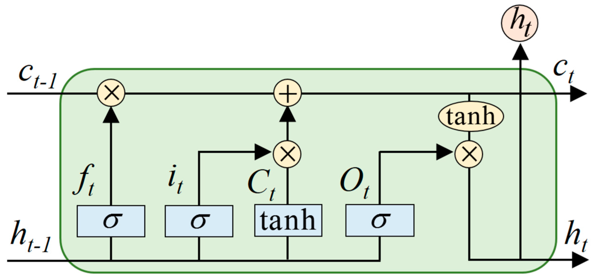
3.1.1. Long Short-Term Memory
3.1.2. Gated Recurrent Units
3.1.3. Convolutional Neural Networks
3.1.4. Transformers
3.2. DL-Based RUL Prediction
3.3. Low-Code Platform Design Concept
4. Software Design
4.1. Software Structure
4.1.1. Software Architecture Selection
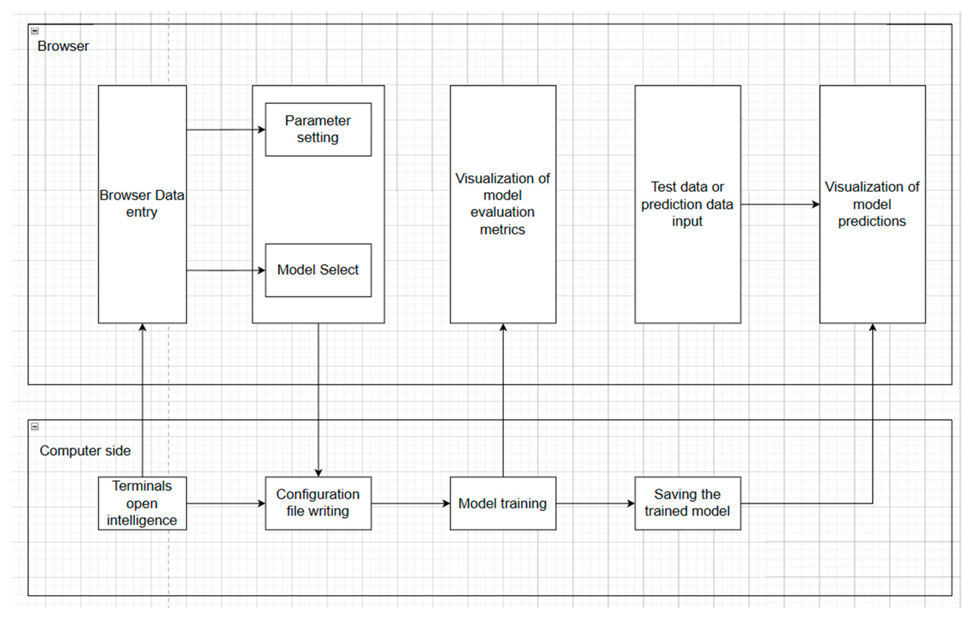
4.1.2. Software Architecture Implementation
4.1.3. Modular Design Principles
4.2. Application Module Details
4.2.1. Interface Interaction Module
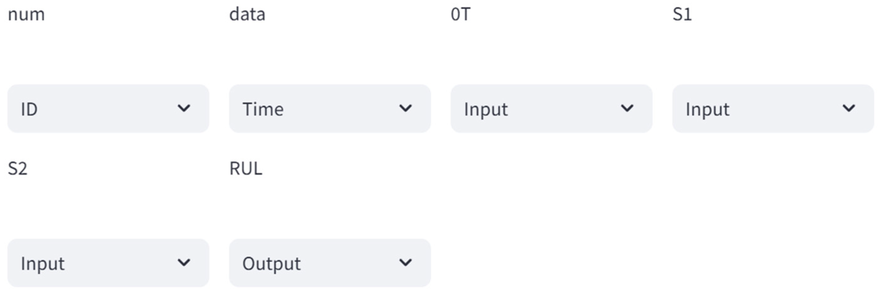
4.2.2. Data Processing Module
4.2.3. Model Selection Module
4.2.4. Visualization Module
5. Software Operation and Practical Examples
5.1. Example Introduction
5.1.1. NASA Turbofan Engine Dataset
5.1.2. HNEI Battery RUL Dataset
5.2. Application Example
5.2.1. Introduction to Evaluation Metrics
5.2.2. NASA Dataset Application
5.2.3. HNEI Battery Dataset Application
5.3. Model Training Efficiency and Resource Requirements
5.4. Comparative Analysis of Model Performance Across Datasets
6. Conclusions
Author Contributions
Funding
Data Availability Statement
Conflicts of Interest
Appendix A
Key Classes, Interfaces, and Functions
References
- Ogunfowora, O.; Najjaran, H. A Transformer-based Framework For Multi-variate Time Series: A Remaining Useful Life Prediction Use Case. arXiv 2023, arXiv:2308.09884. [Google Scholar]
- Li, X.; Ding, Q.; Sun, J.Q. Remaining useful life estimation in prognostics using deep convolution neural networks. Reliab. Eng. Syst. Saf. 2018, 172, 1–11. [Google Scholar] [CrossRef]
- Gao, Z.; Wang, C.; Wu, J.; Wang, Y.; Jiang, W.; Dai, T. Degradation-Aware Remaining Useful Life Prediction of Industrial Robot via Multiscale Temporal Memory Transformer Framework. Reliab. Eng. Syst. Saf. 2025, 262, 111176. [Google Scholar] [CrossRef]
- Wang, L.; Zhao, X.; Pham, H. Novel formulations and metaheuristic algorithms for predictive maintenance of aircraft engines with remaining useful life prediction. Reliab. Eng. Syst. Saf. 2025, 261, 111064. [Google Scholar] [CrossRef]
- Zhou, Y.; Wang, H.; Jin, H.; Liu, Y.; Liu, X.; Cao, Z. Remaining useful life prediction for machinery using multimodal interactive attention spatial–temporal networks with deep ensembles. Expert Syst. Appl. 2025, 263, 125808. [Google Scholar] [CrossRef]
- Kim, M.; Yoo, S.; Son, S.; Chang, S.Y.; Oh, K.-Y. Physics-informed deep learning framework for explainable remaining useful life prediction. Eng. Appl. Artif. Intell. 2025, 143, 110072. [Google Scholar] [CrossRef]
- Chen, Z.; Wu, M.; Zhao, R.; Guretno, F.; Yan, R.; Li, X. Machine Remaining Useful Life Prediction via an Attention Based Deep Learning Approach. IEEE Trans. Ind. Electron. 2020, 68, 2521–2531. [Google Scholar] [CrossRef]
- Cheng, C.; Ma, G.; Zhang, Y.; Sun, M.; Teng, F.; Ding, H. A deep learning-based remaining useful life prediction approach for bearings. IEEE/ASME Trans. Mechatron. 2020, 25, 1243–1254. [Google Scholar] [CrossRef]
- Francisco, O.V.; Rosaria, S. Machine learning for marketing on the KNIME Hub: The development of a live repository for marketing applications. J. Bus. Res. 2021, 137, 393–410. [Google Scholar] [CrossRef]
- Demšar, J.; Zupan, B. Hands-on training about data clustering with orange data mining toolbox. PLoS Comput. Biol. 2024, 20, e1012574. [Google Scholar] [CrossRef]
- Baratchi, M.; Wang, C.; Limmer, S.; van Rijn, J.N.; Hoos, H.; Bäck, T.; Olhofer, M. Automated machine learning: Past, present and future. Artif. Intell. Rev. 2024, 57, 122. [Google Scholar] [CrossRef]
- Kok, C.L.; Tan, H.R.; Ho, C.K.; Lee, C.; Teo, T.H.; Tang, H. A Comparative Study of AI and Low-Code Platforms for SMEs: Insights into Microsoft Power Platform, Google AutoML and Amazon SageMaker. In Proceedings of the 2024 IEEE 17th International Symposium on Embedded Multicore/Many-core Systems-on-Chip (MCSoC), Kuala Lumpur, Malaysia, 16–19 December 2024; pp. 50–53. [Google Scholar] [CrossRef]
- Vaswani, A.; Shazeer, N.; Parmar, N.; Uszkoreit, J.; Jones, L.; Gomez, A.N.; Kaiser, L.; Polosukhin, I. Attention is all you need. arXiv 2017, arXiv:1706.03762. [Google Scholar]
- Kim, Y. Convolutional neural networks for sentence classification. arXiv 2014, arXiv:1408.5882. [Google Scholar]
- Hochreiter, S.; Schmidhuber, J. Long short-term memory. Neural Comput. 1997, 9, 1735–1780. [Google Scholar] [CrossRef] [PubMed]
- LeCun, Y.; Bottou, L.; Bengio, Y.; Haffner, P. Gradient-based learning applied to document recognition. Proc. IEEE 2002, 86, 2278–2324. [Google Scholar] [CrossRef]
- Sutskever, I.; Vinyals, O.; Le, Q.V. Sequence to sequence learning with neural networks. arXiv 2014, arXiv:1409.3215. [Google Scholar]
- Graves, A. Generating sequences with recurrent neural networks. arXiv 2013, arXiv:1308.0850. [Google Scholar]
- Vinyals, O.; Toshev, A.; Bengio, S.; Erhan, D. Show and tell: A neural image caption generator. In Proceedings of the IEEE Conference on Computer Vision and Pattern Recognition, Boston, MA, USA, 7–12 June 2015; pp. 3156–3164. [Google Scholar]
- Wu, H.; Xu, J.; Wang, J.; Long, M. Autoformer: Decomposition transformers with auto-correlation for long-term series forecasting. arXiv 2021, arXiv:2106.13008. [Google Scholar]
- Saxena, A.; Goebel, K. Turbofan Engine Degradation Simulation Data Set. In NASA Prognostics Data Repository; NASA Ames Research Center: Moffett Field, CA, USA, 2008. [Google Scholar]
- Ignavinuales. Battery RUL Dataset [DB/OL]. 1 January 2023. Available online: https://github.com/ignavinuales/Battery_RUL_Prediction (accessed on 11 June 2024).


| Platform/Tool | Advantages | Disadvantages |
|---|---|---|
| KNIME | Strong plugins and functionality, supports multiple data sources, AutoML integration | Steep learning curve, outdated interface, performance bottlenecks with large data |
| Orange | Simple to use, open-source, supports various algorithms | Less powerful than KNIME, limited data processing ability, fewer plugins |
| AutoML (General) | Automated workflows, quick prototyping, reduces human intervention | Low flexibility, black-box issue, high resource consumption |
| Dataset | Number of Training Tracks | Number of Test Trajectories | Fault Pattern |
|---|---|---|---|
| FD001 | 100 | 100 | 1 (HPC degradation) |
| FD002 | 260 | 259 | 1 (HPC degradation) |
| FD003 | 100 | 100 | 2 (HPC degradation, fan degradation) |
| FD004 | 248 | 249 | 2 (HPC degradation, fan degradation) |
| Unit number | Indicates the engine number. |
| Time (period) | Indicates the number of cycles in which the engine is running. |
| Operation settings | Includes three operational setting variables—the flight altitude, throttle analysis angle (TRA), and Mach number. |
| Sensor measurement | The measurements include 21 sensors, such as the total temperature at the fan inlet (T2) and the total temperature at the low-pressure compressor outlet (T24). |
| cycle_index | The number of charge and discharge cycles of the battery is used to reflect its aging process. |
| discharge_time | The time (seconds) it takes for the battery to go from full charge to the set cut-off voltage in a complete discharge cycle is an indicator of health. |
| decrement_3.6–3.4 V | The time (sec) used to reduce the voltage from 3.6 V to 3.4 V is closely related to the voltage attenuation rate in this interval, which is a sensitive feature of the battery degradation process. |
| max_discharge_voltage | The highest voltage value during discharge (usually measured at the beginning of discharge) can be used to understand the decline in battery capacity. |
| min_charge_voltage | The minimum voltage during the charging process (usually measured at the beginning of the charging) reflects the change in the battery state to some extent. |
| time_at_4.15 V | The duration (seconds) that the battery voltage remains within the 4.15 V range reflects the characteristics of the constant voltage phase and can indirectly reveal the characteristics of the internal resistance and capacity of the battery. |
| constant_current_time (TCC) | The time (seconds) when the current is maintained constant during discharge corresponds to the change in the internal electrical characteristics and is often associated with the aging state of the battery. |
| charging_time | The discharge time variation reflects the remaining available capacity in seconds for a full charge cycle. |
| RUL (Remaining Useful Life) | The RUL is the predicted target value of the model. |
| Numerical Visualization of Evaluation Indicators | |
|---|---|
| LSTM | 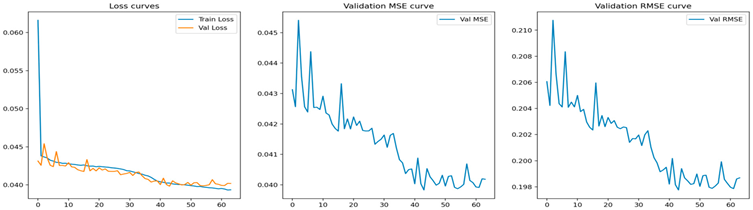 |
| GRU | 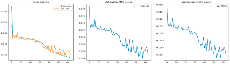 |
| CNN | 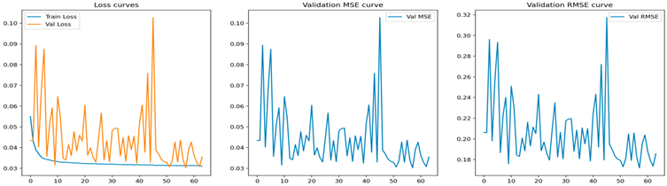 |
| Transformer | 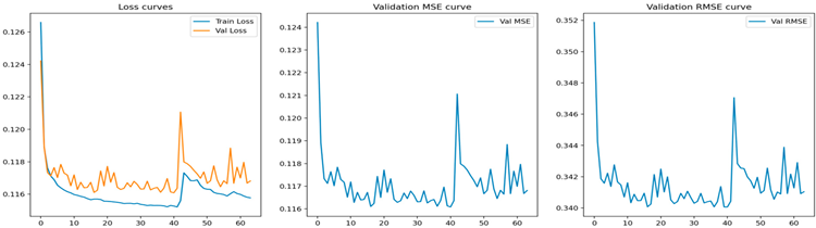 |
| Results of Prediction | Test MSE | Test RMSE | R2 | WMAPE | |
|---|---|---|---|---|---|
| LSTM | 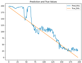 | 0.0136 | 0.1040 | 0.7944 | 0.2052 |
| GRU | 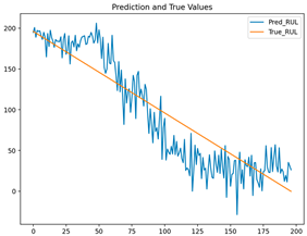 | 0.0299 | 0.1569 | 0.7596 | 0.2306 |
| CNN |  | 0.0209 | 0.1332 | 0.8269 | 0.2051 |
| Transformer | 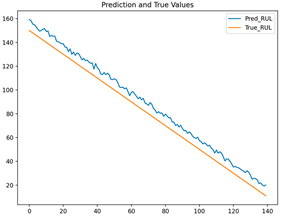 | 0.1485 | 0.3851 | 0.9606 | 0.098259 |
| Numerical Visualization of Evaluation Indicators | |
|---|---|
| LSTM | 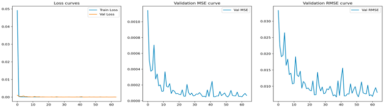 |
| GRU | 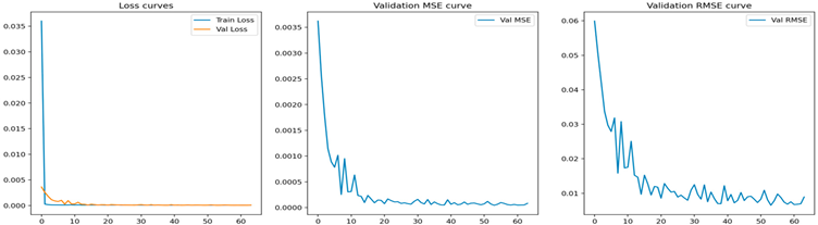 |
| CNN |  |
| Transformer |  |
| Results of Prediction | Test MSE | Test RMSE | R2 | WMAPE | |
|---|---|---|---|---|---|
| LSTM | 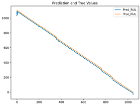 | 0.00029 | 0.0161 | 0.9963 | 0.0348 |
| GRU | 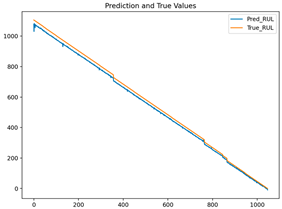 | 0.00022 | 0.0146 | 0.9973 | 0.0244 |
| CNN |  | 0.00014 | 0.0108 | 0.9955 | 0.0379 |
| Transformer | 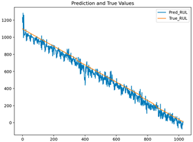 | 0.00167 | 0.0389 | 0.9924 | 0.030296 |
| Model | Dataset | Training Time (s) | Memory Usage (kb) |
|---|---|---|---|
| LSTM | NASA | 2325.80 | 1270 |
| GRU | NASA | 1023.85 | 983 |
| CNN | NASA | 2232.86 | 147 |
| Transformer | NASA | 9305.78 | 6690 |
| LSTM | HNEI | 363.83 | 1315 |
| GRU | HNEI | 549.52 | 987 |
| CNN | HNEI | 312.37 | 149 |
| Transformer | HNEI | 2060.61 | 2997 |
| Model | NASA Test MSE | NASA Test RMSE | HNEI Test MSE | HNEI Test RMSE |
|---|---|---|---|---|
| GRU | 0.0299 | 0.1569 | 0.00029 | 0.0161 |
| LSTM | 0.0136 | 0.1040 | 0.00022 | 0.0146 |
| CNN | 0.0209 | 0.1332 | 0.00014 | 0.0108 |
| Transformer | 0.1485 | 0.3851 | 0.00167 | 0.0389 |
Disclaimer/Publisher’s Note: The statements, opinions and data contained in all publications are solely those of the individual author(s) and contributor(s) and not of MDPI and/or the editor(s). MDPI and/or the editor(s) disclaim responsibility for any injury to people or property resulting from any ideas, methods, instructions or products referred to in the content. |
© 2025 by the authors. Licensee MDPI, Basel, Switzerland. This article is an open access article distributed under the terms and conditions of the Creative Commons Attribution (CC BY) license (https://creativecommons.org/licenses/by/4.0/).
Share and Cite
Lin, Y.; Chen, J.; Chen, S.; Nie, Y.; Wang, M.; Zhang, B.; Yang, M.; Wang, J. A Low-Code Visual Framework for Deep Learning-Based Remaining Useful Life Prediction. Processes 2025, 13, 2366. https://doi.org/10.3390/pr13082366
Lin Y, Chen J, Chen S, Nie Y, Wang M, Zhang B, Yang M, Wang J. A Low-Code Visual Framework for Deep Learning-Based Remaining Useful Life Prediction. Processes. 2025; 13(8):2366. https://doi.org/10.3390/pr13082366
Chicago/Turabian StyleLin, Yuhan, Jianhua Chen, Sijuan Chen, Yunfei Nie, Ming Wang, Bing Zhang, Ming Yang, and Jipu Wang. 2025. "A Low-Code Visual Framework for Deep Learning-Based Remaining Useful Life Prediction" Processes 13, no. 8: 2366. https://doi.org/10.3390/pr13082366
APA StyleLin, Y., Chen, J., Chen, S., Nie, Y., Wang, M., Zhang, B., Yang, M., & Wang, J. (2025). A Low-Code Visual Framework for Deep Learning-Based Remaining Useful Life Prediction. Processes, 13(8), 2366. https://doi.org/10.3390/pr13082366