Comparison of Contact and Non-Contact in Single-Slope Solar Desalination Systems: Experimental Insights and Machine Learning Predictions

Abstract

Solar desalination systems turn saltwater water into freshwater, which helps to overcome water scarcity. In this study, the effects of direct (contact) and indirect (non-contact) interactions with water in solar desalination were evaluated. The emphasis was on changing water depths to better understand the performance variances. Contact systems have a direct interface between thermal absorption materials and water, whereas non-contact systems avoid material–water contact to increase longevity. The experiments at two elevated water depths (3 cm and 4 cm) were conducted in a single-slope solar desalination system. The productivity of both touch and non-contact systems was investigated in June, August, and October 2024 to gather sufficient data for the training and testing of various machine learning models used to predict the distillate. Surprisingly, the non-contact structure system produced 15% and 8% more distillate than the contact system at 3 and 4 cm water depths, respectively. This insightful result will aid in building efficient and sustainable solar desalination technologies. The comparative study gives information on the trade-off between contact and non-contact techniques, with implications for future advances in solar-powered desalination technology. Among all the machine learning techniques, random forest regression achieved the highest coefficient determination (R² train of 0.89 and R² test of 0.95 for the non-contact structure system and R² of train 0.85 and R² test of 0.98 for the contact structure system). Machine learning techniques improve solar desalination by allowing for predictive insights and efficient maintenance, ultimately leading to sustainable water production.

1. Introduction

An essential requirement of a civilized society is the availability of energy and potable water. To drink, perform household tasks, and operate industrial equipment, humans require drinkable water. A large number of people are becoming more urbanized and industrialized every day, which increases the demand for drinkable water. Consequently, groundwater levels are declining due to the increase in freshwater demands [1]. Desalination is utilized to eliminate salt from seawater, which constitutes three-fourths of the Earth’s surface, to attain equilibrium between supply and demand. This is essential due to the abundance of seawater and solar power [2,3]. Water scarcity may find a compelling solution through the solar desalination of saltwater. Solar radiation consists of ultraviolet, visible, and infrared radiation emitted by the sun, which traverses the glass cover and alters in wavelength upon contact with an absorber surface, generating heat, which is conducted to salty water [4]. As the salty water heats up through conduction, it evaporates and then condenses on bottom glass cover surfaces. The inclination of the glass compels the condensed liquid to flow to the tube connected to the shorter side of the solar still, where it is collected in the vessel [5].

In order to enhance the SS’s capacity to absorb solar energy, several low-cost solar absorption materials have been created for use in water to create vapor. A solar still has the potential to improve desalination by utilizing phase-change materials (PCMs). Due to the desalination in plants’ long-term operations, monetary analysis was steered to investigate the yearly productivity of solar stills using shaped and stabilized PCMs [6]. It was revealed that truncated conic fins in solar stills have more distillate yield than regular stills because they transmit more heat to the water around them. When compared to solar stills with only evacuated tubes and solar stills with only calcium stones, the yield obtained by solar stills with both was shown to be the maximum distillate for the entire day as well as at night due to the combination usage of evacuated tubes and calcium stones [7]. Calcium stones are good storage resources for hot water because they captivate heat and increase distillate output in the nig.

The incorporation of magnets in solar stills accelerates the breaking of hydrogen bonds in water, thus enhancing the distillate of water in comparison to conventional solar stills (CSSs) [8]. When considering the enhancement of evaporation and light absorbance, black naphthylamine dye emerges as the optimal choice [9]. Evaporation and output rates are higher in an improved still utilizing nanoparticles (NPs) than in a traditional still. This is because of the enhanced rate of heat exchange and water temperature generated by the presence of NPs. When compared to a traditional solar still, using cuprous oxide particles over the black covering of solar still surfaces yielded a higher distillate [10]. The thermal and physical properties of water nanofluids with varying concentrations of aluminum, zinc, iron, and tin oxides were evaluated, and the most suitable nanofluids were selected for the assessment of the performance in a solar still [11]. The use of different aspect ratios with the same surface and wick materials, such as cooling glass covers and exterior reflectors, to enhance the efficiency of wick solar stills depends on a thorough understanding of the appropriate wick material types and dimensions [12].

The implementation of a black jute wick strap inside the desalination unit, in conjunction with graphene nanofluid quantum dots, significantly enhanced the efficiency of clean water condensation and thermal power [13]. A combined CO₂ power cycle that utilizes geothermal power produces electricity for reverse osmosis desalination, facilitating freshwater generation [14]. Nanostructures that incorporate plasma-improved resonance, wave-guide effect, water surface heat capture, and capillarity enhance the efficiency of solar desalination apparatus. An energy analysis [15] identifies the main power-utilizing component and the amount of electrical energy consumed in the unit.

The conversion of liquid water to vapor using the sun’s energy is known as solar evaporation. Throughout this process, the energy carried by photons originating from the sun is transmitted to molecules in a liquid state. To absorb most solar energy, enormous depths are required [16]. To address this absorption constraint, researchers have utilized a range of solar energy-absorbing materials in their studies, like floating nanostructures. The absorber material has the ability to capture and retain sunlight and then transmits heat energy to water through thermal conduction. In contrast to sunlight’s wavelengths, water readily absorbs infrared (IR) photons. The idea of the NCNS system was established using water’s IR absorption property. Rather than immersing a solar energy-absorbing substance in a liquid, we used thermal down-conversion to convert the sun’s spectrum to thermal infrared radiation. The NCNS system transforms solar energy into heat, and subsequently, it is discharged again as thermal radiation into the water, exhibiting characteristics similar to those of a blackbody. Water molecules have a remarkable IR absorption capability. The uppermost sub100 m layer of water absorbs heat radiation released by the NCNS, transforming the water into its own efficient absorbent [17]. Synthetic saline water was tested at various depths with or without a reflector. Due to the interfacial heating effect of the NCNS, experiments were carried out with and without a reflector, altering the air gap between the non-contact nanostructure and liquid to examine the effect of the air gap on the NCNS system’s production improvement. Independent machine learning (ML) models like ANNs, RFs, and SVRs were used to successfully anticipate the efficiency of a dual-slope solar still. RF was the most efficient method [18]. Several types of artificial neural networks (ANNs) were built and evaluated to see which is the most accurate at forecasting the output and water temperature [19]. Titania–water nanofluid thermal conductivity was evaluated using five ML approaches, each having its own unique set of hyperparameters and logical functions [20].

All the examined solar desalination enhancement methods involving physical coupling with water exhibit limitations in distillate output and fouling resistance. A non-contact nanostructure was employed to surmount the limitations of the direct contact methods. This study conducted solar desalination at greater depths (3 and 4 cm) using a non-contact nanostructure to mitigate fouling constraints. Further, the application of machine learning techniques like linear regression, multiple linear regression, and decision tree and random forest regression were utilized to calculate approximately the output of the solar desalination system at higher depths of water.

2. Non-Contact Nanostructure Development and Experimentation

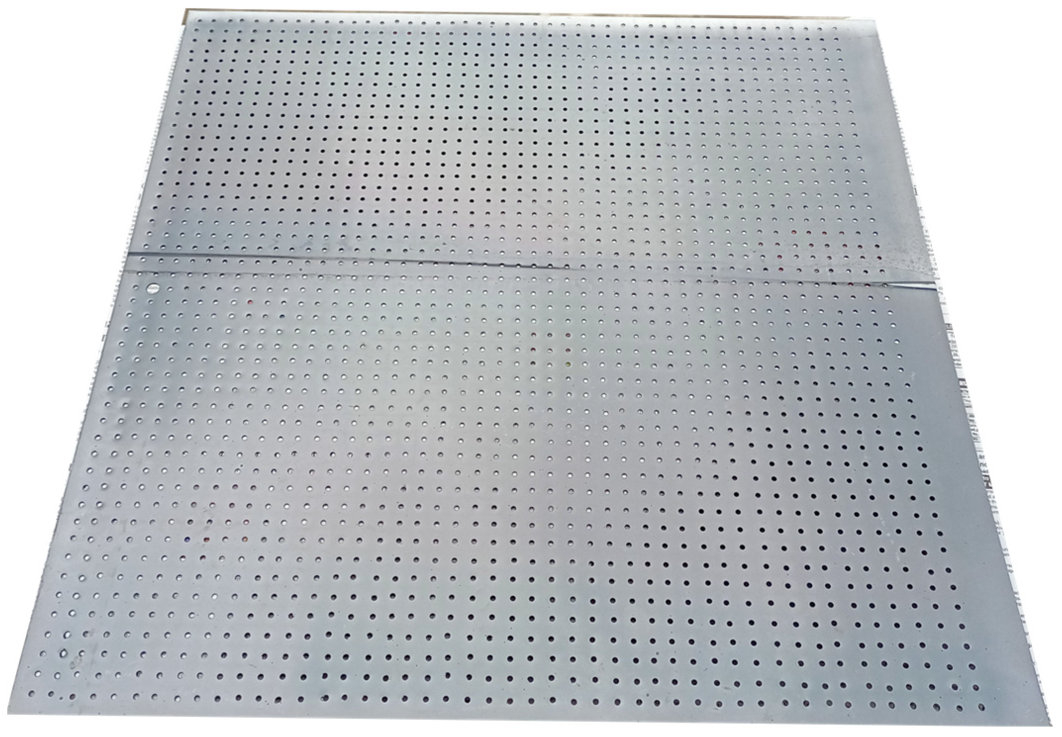
2.1. Fabrication of Perforated Sheet

A square area of 490 × 490 mm² of an SS202 sheet was cut and perforated with circular holes of 1.3 mm in radius with a central space of 10 mm. The thickness of the sheet was 0.8 mm, and 5% of the sheet surface area was made open for the smooth flow of evaporation. The assumption that the NCNS top layer should receive insolation at all times and that there should be sufficient holes of the proper size for water vapor to easily move through the NCNS during evaporation led to the choice of a 5% open area. The hole-making process significantly deformed the sheet, so it had to be straightened using a flattening machine before the polishing process could proceed. The application of the solar selective absorptive coating involved mirror finishing on the perforated sheet, as illustrated in Figure 1.

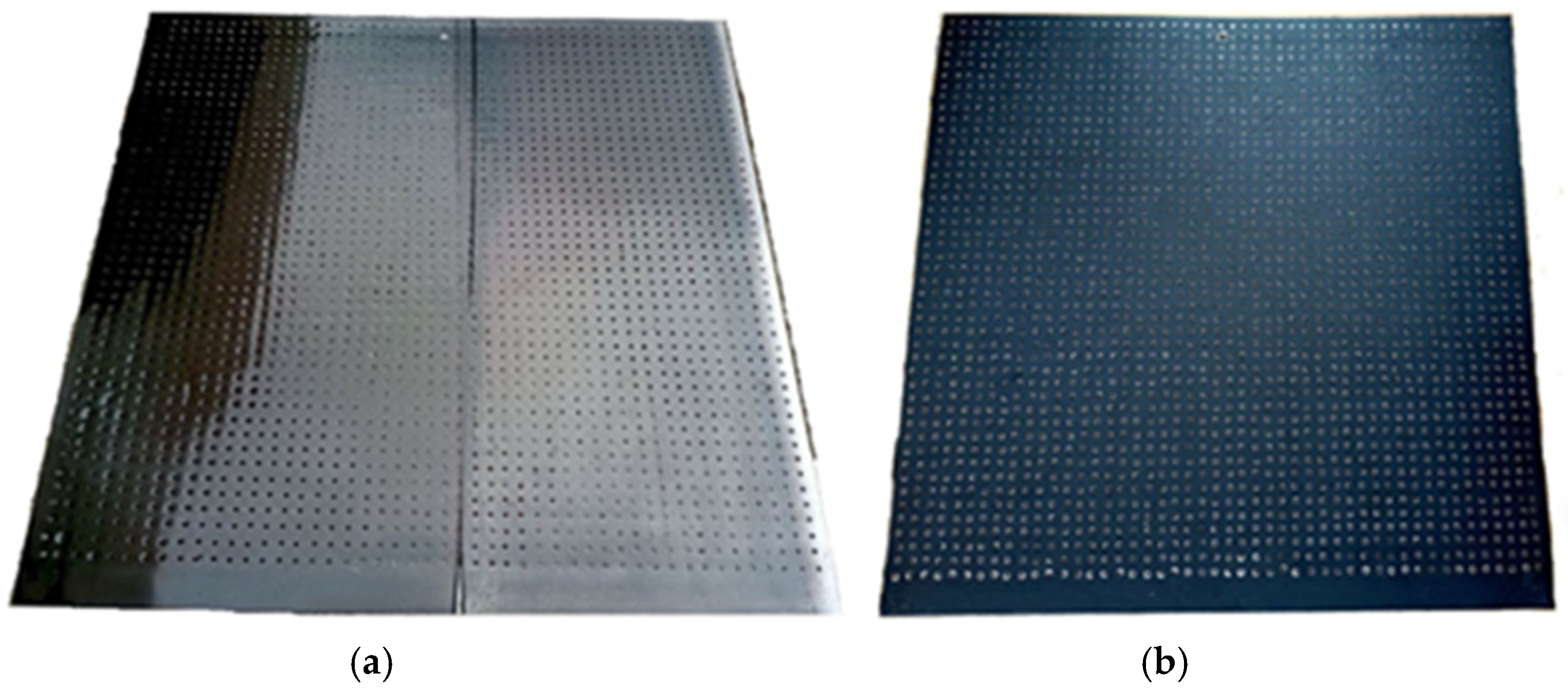
2.2. Fabrication of a Nanocoated Perforated Sheet for Enhanced Absorption

Raw materials like sodium dichromate dihydrate (Na₂Cr₂O₇·2H₂O), secondary propyl alcohol (99%), sulfuric acid (98%), and de-mineralized water were obtained from Merck to develop a nanocoating on the perforated sheet.

By a carefully regulated chemical oxidation process, a solar selective absorber nanocoating was produced on an incredibly reflective mirror-polished SS202 perforated sheet. Stainless steel of type SS202 is the most affordable type available. To develop a highly absorbent nanocoating, a temperature-controlled chemical bath reactor was used with the optimum amount of 1 M (Na₂Cr₂O₇) salt in sulfuric acid and water to prepare the acidic solution. For the chemical oxidation process, the cleansed perforated sheet was submerged in the acidic solution at a temperature of 80–90 °C for close to 30 min. In the course of chemical oxidation, the composition is partially acidic, which oxidizes the atoms of metal on the surface of the sheet to produce a nanoporous composite oxide layer. The color of the perforated sheet became greyish blue with a lustrous appearance following chemical oxidation. The visual representation of all the stages taken to create extremely specialized nanocoatings for absorbers is available in publication [17]. Following the oxidation process, the sheet was clothed in an environmental fiber cloth bathed in isopropyl alcohol to eliminate any leftover contaminants. After that, the sheet was kept in a heated oven at 100 °C for 600 s. The absorptive nanocoating photograph is displayed in Figure 2a.

2.3. Emissive Coating on the Bottom Side of a Perforated Sheet

The upper surface area of a non-contact nanostructure (NCNS) must be extremely absorptive in order for it to absorb the maximum possible solar energy. For heat radiation to transfer the absorbed energy to the water layer, the bottom surface has to be particularly emissive, leading to evaporation. Condensation formed on the glass cover, resulting in distillate accumulation. An absorbent nanocoating was applied to both sides of the punched sheet. The requirement that one side of an NCNS be extremely absorbent and the other extremely emissive was the most difficult to achieve. Even a small amount of emissive coating or absorptive layer may not be on the top or bottom of the NCNS. An emissive surface needs to be created on the bottom side. After sand polishing the bottom side to eliminate the nanocoating, the area was washed with purified water to get rid of any surface-attached dirt. Rust-Oleum’s flat black spray paint, which is readily available, was the paint used to create a surface with a high emissivity. The open area of the absorptive surface was covered with tape while adding the enamel spray for the emissive coating. The shielding covers for the open areas were removed following the spraying process to produce the final NCNS. A picture of the emissive coating is shown in Figure 2b.

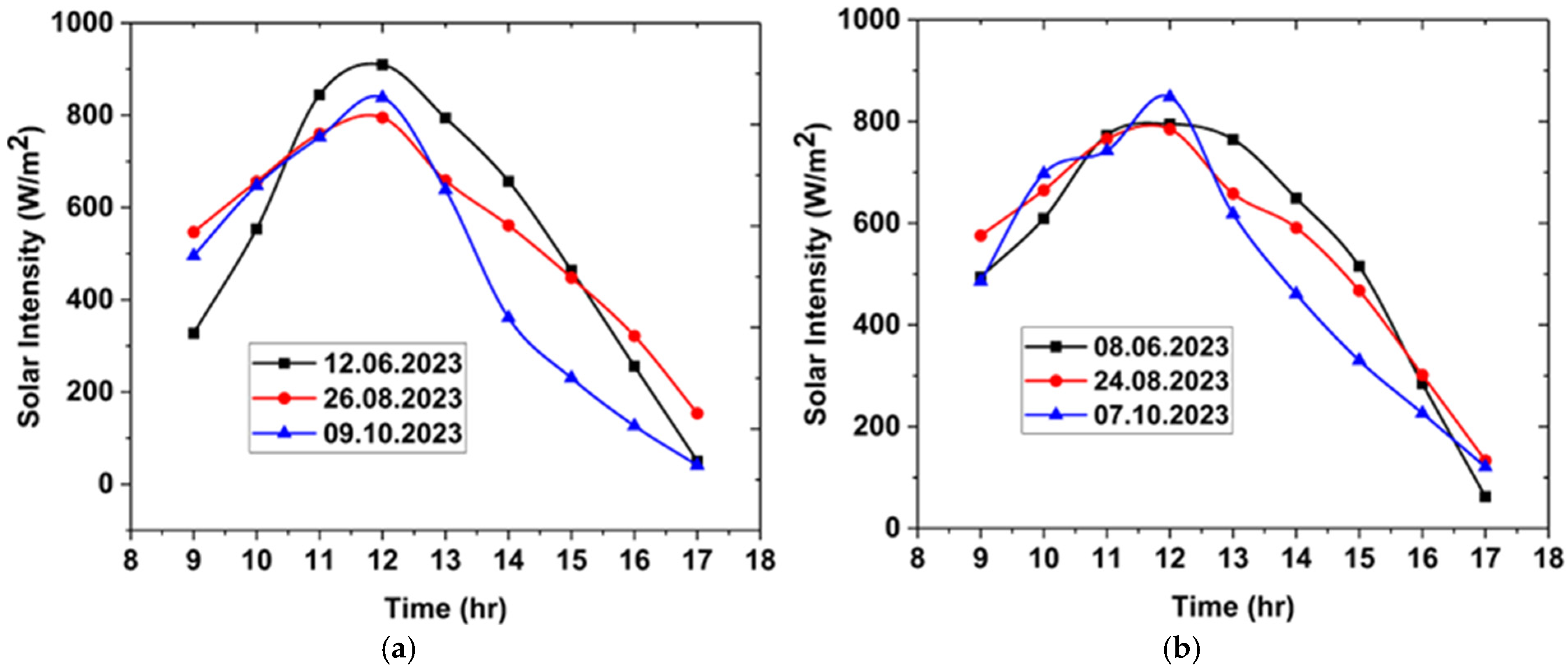
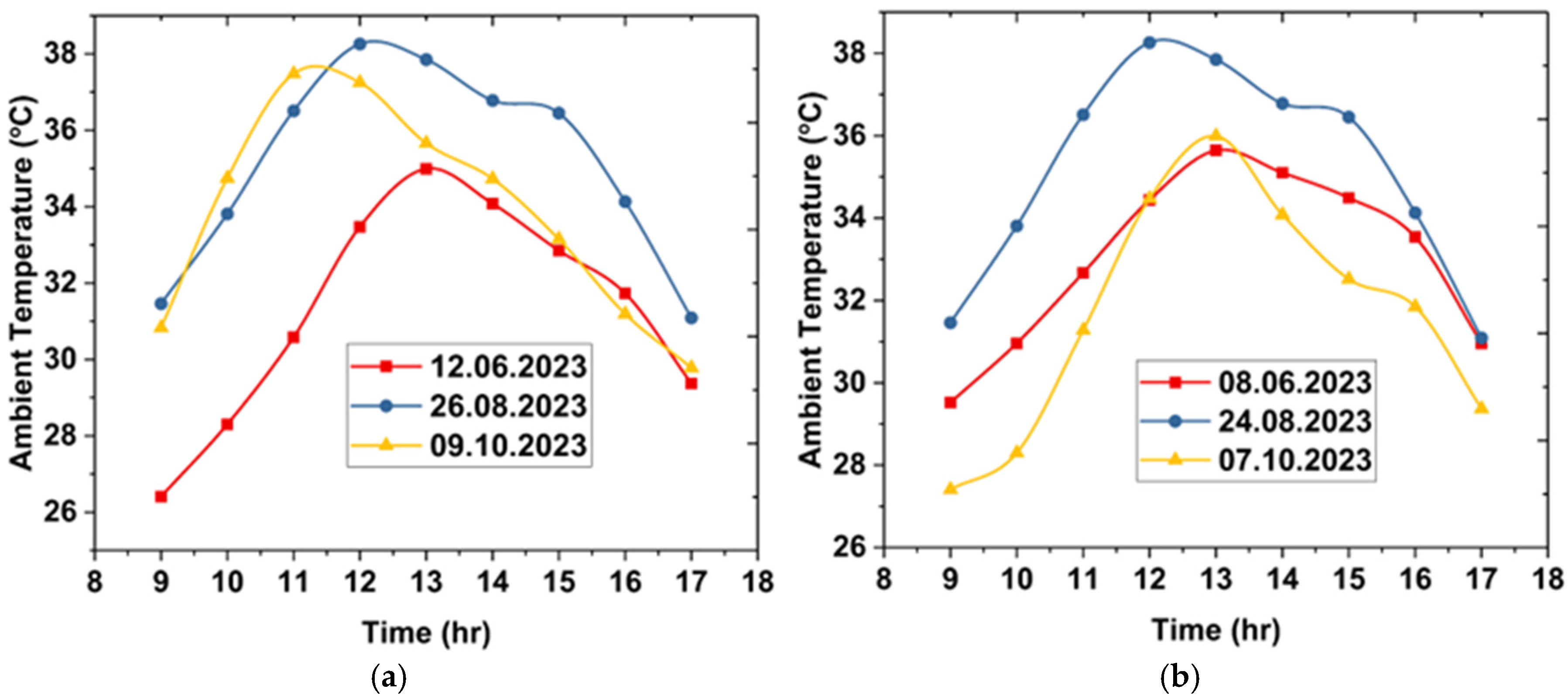
2.4. Experimental Investigation

The one-slope NCNS solar still exterior structure was fabricated using thick plywood of two inches. The external hardwood basin was 54 × 54 cm. The leading height was 20 cm, and the rear measured 37 cm. The external structure was designed to inhibit heat loss into the environment and segregate heat flow. The exterior component functions to insulate heat transfer and was built to avert thermal loss to the environment. The NCNS interior structure was fabricated from 1 mm thick galvanized iron. The basin surface area of the interior structure was 2500 cm², featuring a black powder coating. The schematic diagram is shown in Figure 3. The elevation of the back side was 35 cm, while for the shorter side, it was 18.8 cm. A galvanized pipe with a diameter of 0.635 mm was welded to the rear of the SS to facilitate the ingress and egress of seawater. The shorter side involves affixing a glass cover of 52 × 54 × 0.4 cm dimensions to the apex of the SS structure. The heights of the NCNS were changed using plastic rods measuring 4.5 cm in height. Polyimide tape possessing a thermal conductivity of 0.12 W/m-k was employed to encase the edges of the NCNS, and after that, the NCNS was positioned on the acrylic rods and adhered using adhesive. A strip of double-sided tape was affixed to the upper edges of the SS. Once the glass was securely affixed to the tape, silicone adhesive was applied in the space between the glass and tape to prevent water vapor from escaping. Silicone adhesive was also employed to seal the space between the upper short side and the glass shield of the solar still, enhancing its integrity. A half-circular duct connected to the smaller side of the SS catches the condensed distilled water that accumulates on the glass (Mohiuddin et al. 2022 [17]). To monitor the various temperatures of the water, glass, basin, and NCNS, K-type thermocouples were installed. The K-type thermocouples were linked to the data acquisition (DAQ) system for temperature reading and logging. The intensity of sunlight and ambient temperature was quantified and logged with a pyranometer. For a depth of 4 cm, 10 liters of water were introduced into the solar stills, and for a depth of 3 cm, 8.75 liters of water were utilized in both the CSS and the NCNSSS. The experiment commenced at 9 a.m. and concluded at 5 p.m. Temperature values and distillate production measurements were recorded every thirty minutes. The measurements of the NCNS and CSS systems were recorded to compare one with the other. Configurations were made in the DAQ system to record temperature data at one-minute intervals. These data were utilized for machine learning methodologies. Figure 4 depicts the non-contact nanostructure solar still (NCNSSS) and the conventional solar still (CSS).

2.5. Uncertainty Analysis

The distinction between true values and estimated values, referred to as error, constitutes the fundamental aspect of uncertainty analysis. Ambiguity errors can be classified into two distinct categories. Mathematical analysis and systematic research methodologies can effectively quantify type A errors, which are classified as random errors. Data books and equipment calibration reports are capable of identifying type B errors, which are classified as systematic errors. The mathematical expression presented below enables the derivation of conclusions pertaining to the standard uncertainty:

$$\mathrm{u}=\mathrm{a}/\sqrt{3}$$

(1)

Here, “u” is the standard uncertainty, and “a” is the accuracy of the measurement apparatus.

The inherent instrumental uncertainties of the measuring procedure were the primary focus of the experimental investigation. The instrumental uncertainties caused a daily fresh water productivity margin of error of ±1.5%. In order to gather trustworthy data, this part of the analysis stressed the significance of using precise equipment and measurement methods. In addition to the issues already mentioned, the investigation encountered new ones while trying to measure solar radiation and system temperatures. These uncertainties are crucial study variables because they affect the performance of solar stills.

Table 1. Range of operation and precision of the utilized instruments.

S. No.	Device	Precision	Range	Uncertainty
1	Pyranometer	±5 W/m2	0–1600 W/m2	±0.36
2	Thermocouple	±1 °C	0–500 °C	±0.12
3	Anemometer	±0.5 m/s	0–30 m/s	±0.20

shows the precision, range, and relative uncertainty of the utilized instruments. Figure 5 portrays the relative uncertainties of the various instruments utilized.

3. The Significance of Machine Learning

Machine learning is of essential relevance in today’s digital age, as it transforms the way we analyze and extract meaningful insights from massive volumes of data. It empowers organizations and sectors across the board by automating decision-making processes, boosting predictive skills, and streamlining operations. Machine learning algorithms help us to find hidden patterns, generate precise estimations, personalize user experiences, and tackle previously intractable and complicated challenges. Machine learning is at the vanguard of innovation, driving efficiency, and changing how we leverage data to improve our lives and drive development in the modern world, from healthcare to finance and self-driving automobiles to recommendation systems. ML models estimate the potential fresh water yield of a solar desalination system under certain conditions, resulting in time and cost savings on testing. By optimizing performance and preventing unnecessary energy use, machine learning paves the way for sustainable, cost-effective desalination.

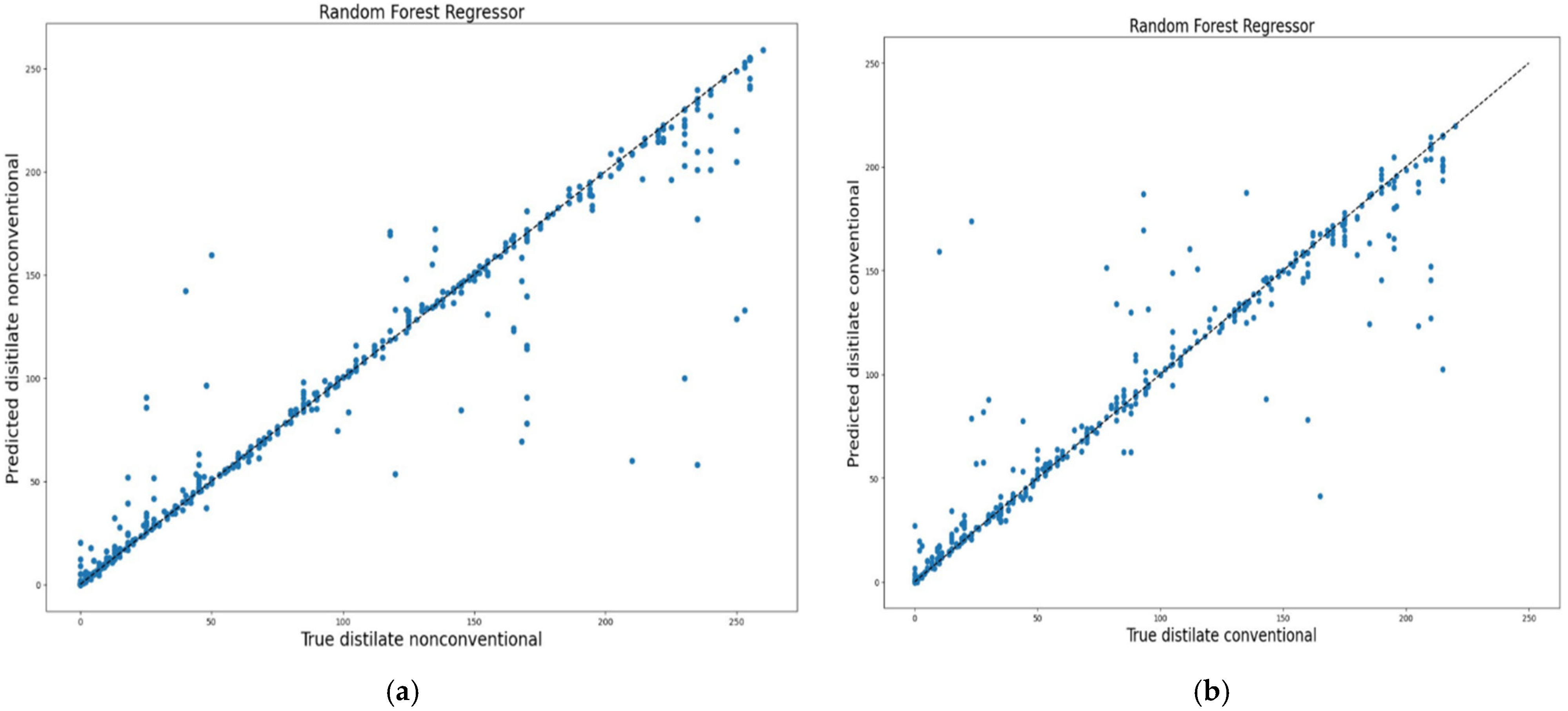
3.1. Random Forest Regression

Random forest is a “tree”-based approach that generates options through merging the features from multiple decision trees. The word “random” alludes to the algorithm’s “randomly generated decision trees” forest [21]. Each decision tree is trained on a random collection of characteristics in addition to various types of data. This contributes to tree diversity and prevents any particular trait from dominating estimations. When making predictions, each decision tree in the random forest guesses the target value independently. The predictions from all the trees are then averaged to generate the final ensemble prediction for regression tasks. Predictions from numerous decision trees are more stable and reliable than predictions from a single tree. This averaging approach helps to level out the biases and inaccuracies of individual trees. Overfitting is a serious flaw in the decision tree. Using a random forest instead of a decision tree can prevent overfitting. The model’s consistency is ensured via tree variety. There are two methods for cultivating trees: randomly choosing predictor subsets and sampling with substitution. This utilizes a randomly selected sample of data that has been created. Data utilized as a training subset are referred to as “in-bag” data, while the rest are referred to as “out-of-bag” data. Without the requirement for a separate validation set, these out-of-bag data can be utilized to estimate the model’s performance [22].

3.2. Linear Regression

Linear regression is an analytical technique that utilizes observed data points to establish a linear equation that signifies the relation between several independent variables and a dependent variable. The technique is for determining a line of the ideal fit that reduces the variation between the expected outcomes from the equation and the actual data points [23]. The least squares method reduces the sum of squared variances among anticipated and actual outcomes. The resulting equation depicts the linear connection among variables, conceding for the prediction and comprehension of how variations in independent factors affect the dependent variable.

Linear regression can be shown mathematically as:

Y = aX + b

(2)

where a and b are linear coefficients, Y is dependent (predictor), and X is independent (goal).

3.3. Multiple Linear Regression

Multiple linear regression is a primary statistical and machine learning technique for modeling correlations between many predictor variables and a continuous target variable. This strategy’s goal is to find the best-fitting linear equation that explains how changes in the predictor variables affect changes in the target variable [23]. Each predictor variable is assigned a value called the coefficient, which represents its effect on the desired variable while accounting for other predictors. By evaluating the coefficients of the variables that are independent in this equation, based on predictor values, the model can calculate the dependent variable:

Y = b₀ + b₁x₁ + b₂x₁

(3)

• Y = response variable;
• b₀, b₁, b₂, b_3, b_n… = model coefficients;
• x₁, x₂, … = feature variables.

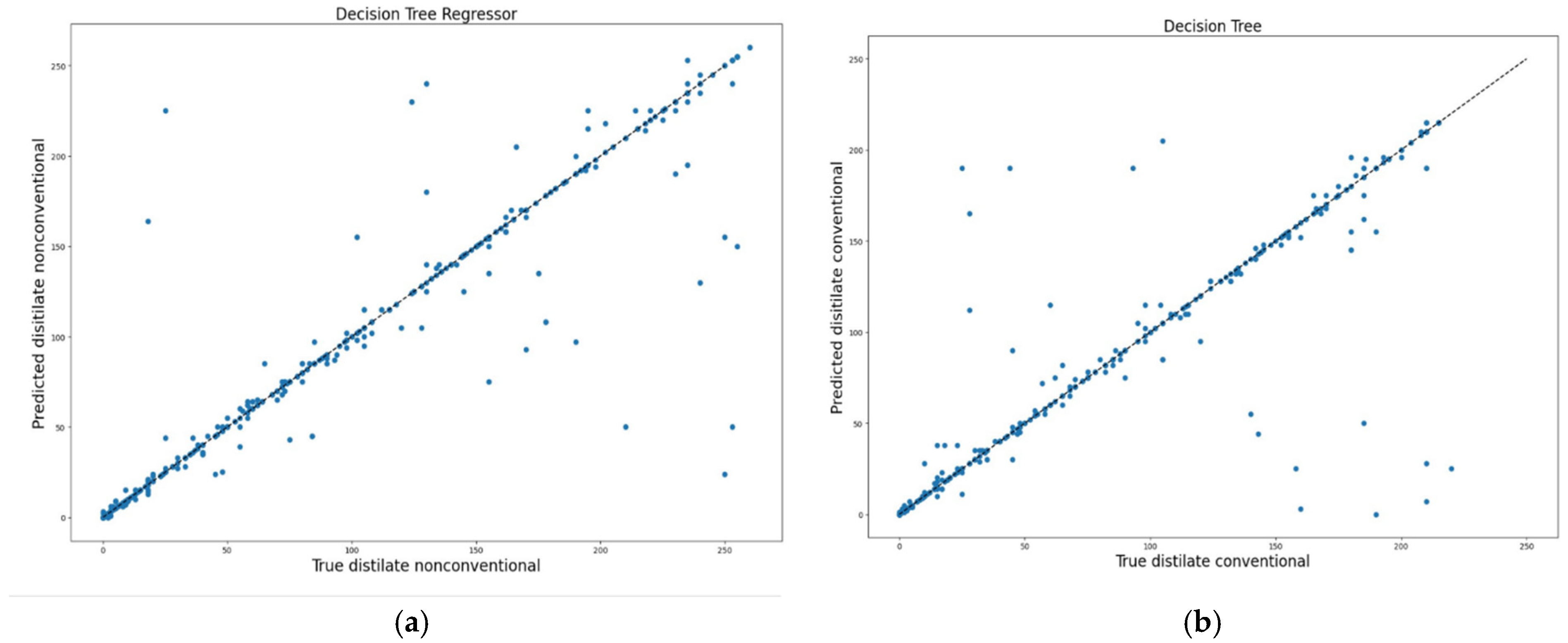
3.4. Decision Tree

One of the functional methods that is most frequently used is the decision tree (DT) method of performing supervised learning. Although it can tackle classification and regression issues, the latter are more frequently encountered. It is a classifier with a three-type node tree topology. The sample’s initial node’s root node is the principal identifier. The tree can be decomposed into nodes. The leaf nodes denote the outcome, the inside nodes denote the characteristics of data collection, and the branching characterizes the decision rules. Decision-making problems can be solved with the help of this algorithm. In this work, one point of data was traversed across the entire tree by answering true or false queries before reaching the leaf node. The choice of performing tactical splits greatly impacts the precision of a tree. The requirements for selecting trees for regression and classification varied [20].

DTR frequently uses MSE (mean square error) to divide a node into more than one subnode. If a binary tree is utilized, the program will initially select a value and then divide the data into two subsets. It calculates the MSE for each subgroup separately. The tree chooses the value that yields the mean squared error. The benefits of adopting a DT include a simplified understanding of the mechanism, a reduced need for data cleaning, and few hyper-parameters to modify. Figure 6 describes a flowchart that visually outlines the sequence of machine learning techniques applied in the study.

4. Results and Discussions

4.1. Technical Assessment

The experiments were conducted utilizing groundwater across three separate months of June, August, and October 2023, with varying water levels of 3 cm and 4 cm. The experimentation for the NCNS and the CSS were executed concurrently. Figure 7 illustrates the correlation between sun intensity and time. The peak insolation of 909.5 W/m² at a 3 cm water level was documented on 12 June 2023 at 12:00 p.m., while the highest recorded values on 9 October and 26 August were 838.25 and 794.82 W/m², respectively, at the same time of the day. The peak sun intensity of 848.25 W/m² for a 4 cm water depth was observed on 7 October 2023 at 12:00 p.m., while the greatest values of 795.11 W/m² and 784.82 W/m² were noted on June 8 and August 24, respectively. The maximum average sunlight intensity at 3 cm of water depth is 847.53 W/m², whereas at 4 cm, it is 809.39 W/m².

Figure 8 illustrates the fluctuation of ambient temperatures. The maximum recorded ambient temperature of 42 °C was seen on 12 June at 3 p.m. for 3 cm level of water, while the maximum logged ambient temperature of 45 °C was noted on 24 August at 2 p.m. for 4 cm water level.

Figure 9 illustrates the variation in NCNS system temperatures over the period of three days, with each day of different months for a 3 cm water level. Figure 10 depicts the variation in NCNS system temperatures over time for a 4 cm water level across three days, with each day of a different month. In all instances, the absorber temperature was elevated at 2 p.m. due to the peak insolation. The absorber generally comprises a material with elevated solar absorptivity. This indicates its capacity to efficiently absorb sun radiation and convert it into heat. The absorber is designed to effectively trap solar radiation, resulting in a subsequent increase in temperature. The increased temperature is crucial for the desalination process, which often involves the vaporization of water. The basin temperature is the minimum among all temperatures. Upon heating of the absorber, the emitter (absorber bottom side) releases infrared radiation (IR), which is readily absorbed by the topmost stratum of water, measured in micrometers. Infrared radiation preferentially heats the surface water, whereas convection enables the heat transfer from the top to the lower layers. Conduction is the mechanism via which heat is transported from the water’s bottom surface to the basin liner, leading to a heating consequence. It exhibits a consistent style in temperatures at both water depths.

Figure 11 illustrates the variations in CSS temperatures over time for a 3 cm water level across three days, with each day being from a different month, whereas Figure 12 depicts the variations in CSS temperatures over time for a 4 cm depth of water for three days, with each day being from a different month. The basin temperature represents the maximum value in the CSS at 2 p.m., whereas the temperature of the glass denotes the minimum value, as water in the basin of a CSS system demonstrates considerable thermal inertia. This results in a postponement of reaching the maximum water temperature and, subsequently, the glass cover temperature.

Figure 13 illustrates the fluctuations of fresh water production over time at a 3 cm water depth for three days, with each day being from a different month for both desalination systems. The peak production was documented on 12 June 2023 for each system. The peak fresh water production rate occurred between 1 P.M. and 3 P.M. due to elevated insolation.

Figure 14 illustrates the fluctuations of fresh water production over time for a 4 cm water level for three days, with each day being from a different month for both desalination systems. The peak fresh water production was reported on 24 August 2023 for each system. The peak production rate was observed between 1 p.m. and 3 p.m. as a result of increased insolation. The augmentation of water depth in a non-contact nanostructure system yields greater distillate compared to a typical conventional system. At 3 cm and 4 cm water levels, it produces distillate yields that are 15% and 8% more than those of the CSS system, respectively.

4.2. Prediction by Machine Learning Techniques

This study aimed to forecast the distillate output by considering input parameters like still temperatures, time, solar intensity, and ambient temperature. The predictive models employed in this work underwent multiple iterations to provide reliable and precise outcomes. Figure 15 shows the Pearson correlation coefficients between 12 variables related to a solar still. The variables include various sensor readings, temperatures, and insolation. The spectrum ranging from blue to red signifies the intensity of the correlation, with blue signifying negative, white signifying no, and red signifying positive correlations. The correlation matrix provides insights into the relationships between various parameters in a solar still system. A strong positive correlation is observed between glass temperature (non-conventional) and vapor temperature (non-conventional) (0.93), indicating that as the glass temperature increases, the vapor temperature rises correspondingly. Similarly, basin temperature (conventional) and water temperature (conventional) (0.96) show a near-perfect correlation, highlighting that water temperature is highly dependent on basin temperature in a conventional setup. Additionally, the distillate output from conventional and non-conventional systems (0.99) is almost identical, suggesting both setups produce similar results. Moderate correlations exist between ambient temperature and various temperature parameters (0.75–0.84), signifying its influence on system temperatures.

Figure 16 shows the variations between true values and prediction values. The RFR has coefficients of determination for R² training of 0.89 and R² testing of 0.95 for the NCNS system and R² training of 0.85 and R² testing of 0.98 for the CSS system, respectively, and quantifies the percentage of dependence variability determined by independent variables. Given the circumstances, the R² values indicate that the model successfully catches high irregularity in the target variable. It indicates the good fit of the model.

Figure 17 shows the variations between true values and prediction values. The decision tree regression has coefficients of determination for R² training of 0.85 and R² testing of 0.64 for the NCNS system and R² training of 0.78 and R² testing of 0.58 for the CSS system, respectively. The decision tree regression model accounts for approximately 64.80% and 58.51% of the irregularity in the target variable on the test set. The R² values indicate that the model successfully catches moderate irregularity in the target variable. It indicates a better fit for the model.

Figure 18 shows the variations between true values and prediction values. Linear regression has coefficients of determination for R² training of 0.63 and R² testing of 0.69 for the NCNS system and R² training of 0.59 and R² testing of 0.55 for the CSS system. The R² score quantifies the proportion of variability in the variable being investigated that can be explained by the model of linear regression. Here, an R² score signifies that the model takes into consideration around 69% of the variation in the target variable for the NCNS and 55% of the variation in the target variable for the conventional system. It indicates a moderate level of fit. However, the model does not encompass all the varieties that exist.

Figure 19 shows the variations between true values and prediction values. Multiple linear regression has coefficients of determination for R² training of 0.63 and R² testing of 0.62 for the NCNS system and R² training of 0.59 and R² testing of 0.64 for the CSS system. The R² score quantifies the fraction of the variance in the target variable that can be explicated by the model. It suggests a reasonable level of fit. Linear and multiple linear regression fails to capture the full variability in the data, indicating that the relationship between input variables and output is likely nonlinear. However, the model lacks the ability to fully account for a certain level of variability. The multiple linear regression model exhibits coefficients of determination (R²) of 0.63 for training and 0.62 for testing in the NCNS system, while for the CSS system, the model yields an R² of 0.59 during training and 0.64 during testing. The R² score quantifies the proportion of variance in the dependent variable that is explained by the model, indicating a moderate predictive capability. These results suggest that the model effectively captures a significant portion of the variability in the target variable, demonstrating a reasonable level of fit. However, the discrepancy between the training and testing scores, along with the less-than-optimal R² values, implies that the model does not fully account for all sources of variability, potentially due to underlying nonlinearities, unaccounted external factors, or limitations in feature representation.

After the training and testing of all machine learning techniques, random forest regression had a greater level of accuracy and a high coefficient of determination (R²) value because the temperature data in a solar desalination system have nonlinear correlations. The random forest regression (RFR) algorithm is adept at capturing nonlinear patterns in the data because it consists of an ensemble of decision trees. This ensemble approach enables it to effectively describe complicated relationships. Through the process of combining the forecasts of numerous decision trees, it has a tendency to exhibit superior generalization and is less susceptible to overfitting. It is more resilient to outliers because of the smoothing effect produced by several trees. Random forest regression is capable of capturing interaction effects between characteristics, which is particularly important in systems such as solar desalination. In these systems, the influence of temperature on different components may not be easily predictable and can be influenced by the interplay of numerous elements.

RFR can automatically identify significant features by assessing their impact on the overall model performance. This can be advantageous when working with data that have a large number of dimensions. Typically, it is less susceptible to overfitting in comparison to a solitary decision tree. Linear regression and multiple linear regression may still be suitable for scenarios where the relationship between variables is approximately linear and assumptions are met. In the temperature dataset, if there are interrelated characteristics (multicollinearity), linear regression models might be affected by this, resulting in unstable coefficient estimations. The models are very responsive to outliers, and even a single outlier can exert a substantial influence on them when compared to RFR. A decision tree consists of a single decision tree that struggles with highly complex data compared to RFR. Hence, RFR is the best method among other machine learning techniques for temperature datasets and characteristics. A comparative statistical analysis of the test and training sets is shown in

Table 2. Comparative statistical analysis of the test and training datasets for machine learning techniques.

Machine Learning Techniques	Type of System	R2 (Training)	R2 (Testing)
Random forest regression	NCNS system	0.89	0.95
	CSS system	0.85	0.98
Decision tree	NCNS system	0.85	0.64
	CSS system	0.78	0.58
Linear regression	NCNS system	0.63	0.69
	CSS system	0.59	0.55
Multiple linear regression	NCNS system	0.63	0.62
	CSS system	0.59	0.64

. The solar desalination process is inherently multivariable and nonlinear due to its dependence on temperature gradients, humidity, heat transfer modes, environmental factors, and system design. Machine learning models like random forest perform well because they capture these complex interactions, whereas simpler models like linear regression struggle due to the highly nonlinear dependencies. The random forest regression model exhibits the highest R² scores across both training and testing for NCNS (0.89 and 0.95) and CSS (0.85 and 0.98) systems. The minimal gap between the training and testing R² indicates strong generalization capability and a low risk of overfitting. This suggests that random forest is well-suited for capturing complex relationships in solar still systems due to its ensemble-based learning.

5. Conclusions

The trials were carried out to investigate the correlation between solar intensity, ambient temperature, and still temperature for varying water depths in the NCNS and CSS systems. The experiments were conducted with tap water during the three specific months of June, August, and October 2023. Various water levels, including 3 cm and 4 cm, were utilized. The experimentation for the NCNS and CSS systems was carried out at the same time.

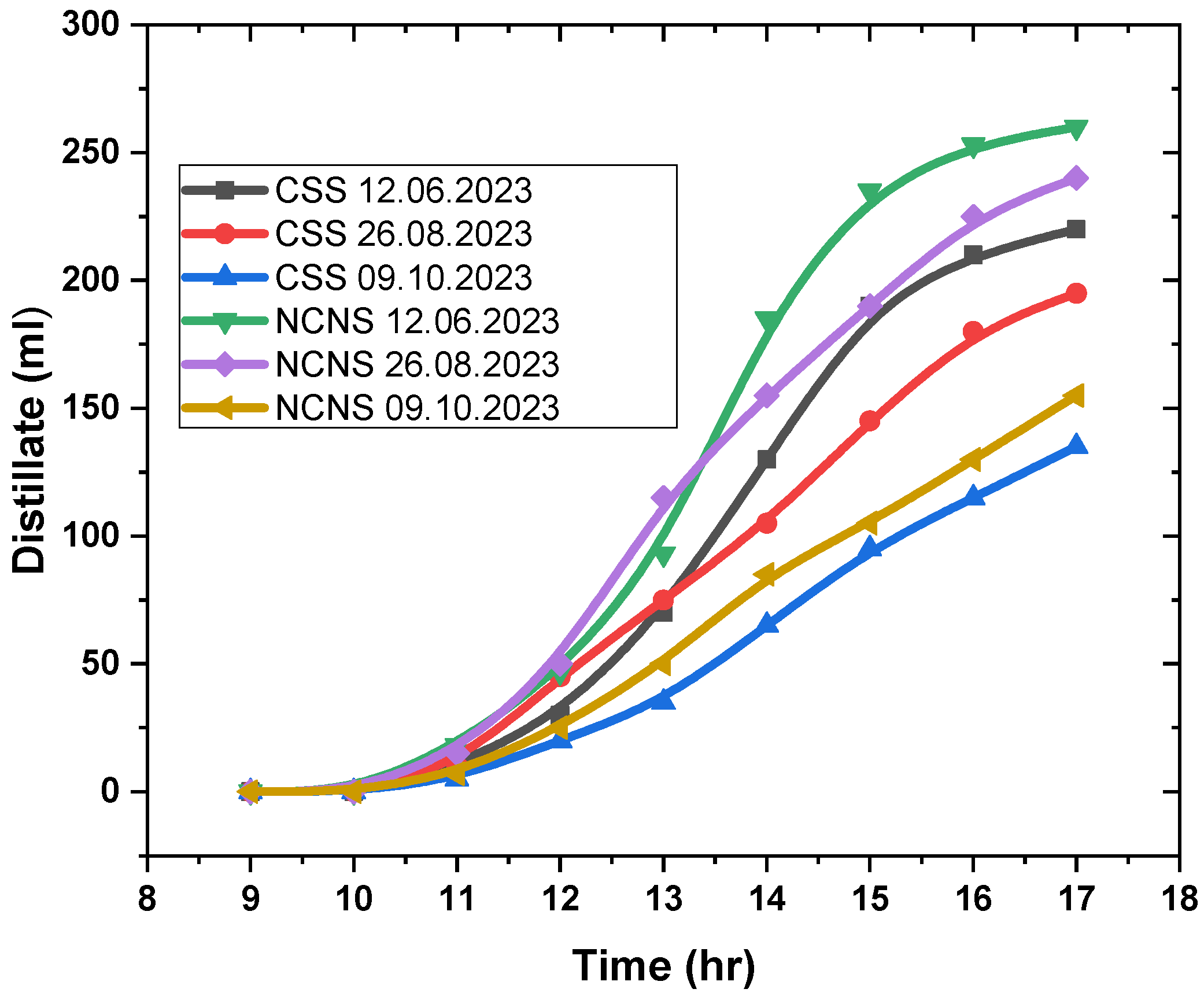
• At greater water levels, the NCNS system showed superior fresh water production than the CSS system;
• For 3 and 4 cm water levels, the NCNS system achieved 15% and 8% higher distillate than the CSS system;
• The maximum fresh water production was logged on 24-08-2023 for both systems, with the highest production rate logged from 1 p.m. to 3 p.m.;
• Random forest regression (RFR) showed higher accuracy and a high R² value in capturing high variability in the target variable;
• The decision tree regression (DTR) model accounts for approximately 64.80% and 58.51% of the irregularity in the target variable on the test set;
• The linear regression model accounts for around 69% of the variation in the target variable for the NCNS system and 55% of the variation in the target variable for the conventional system;
• Random forest performs best but is computationally demanding and lacks interpretability;
• Decision trees overfit and are unstable with small data variations;
• Linear and multiple linear regression fail to capture nonlinear dependencies, limiting their predictive power;
• Feature engineering, better data preprocessing, and advanced models like neural networks or hybrid AI approaches could improve accuracy;
• More data can be generated by conducting year-round experiments;
• Advanced machine learning techniques can be applied to achieve better predictivity.

References

1. Raihananda, F.A.; Philander, E.; Lauvandy, A.F.; Soelaiman, T.A.F.; Budiman, B.A.; Juangsa, F.B.; Sambegoro, P. Low-cost floating solar still for developing countries: Prototyping and heat-mass transfer analysis. Results Eng. 2021, 12, 100300. [Google Scholar] [CrossRef]
2. Xu, Z.; Zhang, L.; Zhao, L.; Li, B.; Bhatia, B.; Wang, C.; Wilke, K.L.; Song, Y.; Labban, O.; Lienhard, J.H.; et al. Ultrahigh-efficiency desalination: Via a thermally-localized multistage solar still. Energy Environ. Sci. 2020, 13, 830–839. [Google Scholar] [CrossRef]
3. Ahmed, F.E.; Hashaikeh, R.; Hilal, N. Solar powered desalination—Technology, energy and future outlook. Desalination 2019, 453, 54–76. [Google Scholar] [CrossRef]
4. Selvaraj, K.; Natarajan, A. Factors influencing the performance and productivity of solar stills—A review. Desalination 2018, 435, 181–187. [Google Scholar] [CrossRef]
5. Kaviti, A.K.; Akkala, S.R.; Sikarwar, V.S.; Sai Snehith, P.; Mahesh, M. Camphor-soothed banana stem biowaste in the productivity and sustainability of solar-powered desalination. Appl. Sci. 2023, 13, 1652. [Google Scholar] [CrossRef]
6. Nian, Y.L.; Huo, Y.K.; Cheng, W.L. Study on annual performance of the solar still using shape-stabilized phase change materials with economic analysis. Sol. Energy Mater. Sol. Cells 2021, 230, 111263. [Google Scholar] [CrossRef]
7. Panchal, H.; Hishan, S.S.; Rahim, R.; Sadasivuni, K.K. Solar still with evacuated tubes and calcium stones to enhance the yield: An experimental investigation. Process Saf. Environ. Prot. 2020, 142, 150–155. [Google Scholar] [CrossRef]
8. Kaviti, A.K.; Ram, A.S.; Thakur, A.K. Influence of fully submerged permanent magnets in the evaluation of heat transfer and performance analysis of single slope glass solar still. Proc. Inst. Mech. Eng. Part A J. Power Energy 2022, 236, 109–123. [Google Scholar] [CrossRef]
9. Rajvanshi, A.K. Effect of various dyes on solar distillation. Sol. Energy 1981, 27, 51–65. [Google Scholar] [CrossRef]
10. Kabeel, A.E.; Omara, Z.M.; Essa, F.A.; Abdullah, A.; Arunkumar, T.; Sathyamurthy, R. Augmentation of a solar still distillate yield via absorber plate coated with black nanoparticles. Alex. Eng. J. 2017, 56, 433–438. [Google Scholar] [CrossRef]
11. Elango, T.; Kannan, A.; Kalidasa Murugavel, K. Performance study on single basin single slope solar still with different water nanofluids. Desalination 2015, 360, 45–51. [Google Scholar] [CrossRef]
12. Sharshir, S.W.; Salman, M.; El-Behery, S.M.; Halim, M.A.; Abdelaziz, G.B. Enhancement of solar still performance via wet wick, different aspect ratios, cover cooling, and reflectors. Int. J. Energy Environ. Eng. 2021, 12, 517–530. [Google Scholar] [CrossRef]
13. Essa, F.A.; Omara, Z.M.; Abdullah, A.S.; Kabeel, A.; Abdelaziz, G. Enhancing the solar still performance via rotating wick belt and quantum dots nanofluid. Case Stud. Therm. Eng. 2021, 27, 101222. [Google Scholar] [CrossRef]
14. Hoseinzadeh, S.; Yargholi, R.; Kariman, H.; Heyns, P.S. Exergoeconomic analysis and optimization of reverse osmosis desalination integrated with geothermal energy. Environ. Prog. Sustain. Energy 2020, 39, e13405. [Google Scholar] [CrossRef]
15. Kariman, H.; Hoseinzadeh, S.; Heyns, P.S. Energetic and exergetic analysis of evaporation desalination system integrated with mechanical vapor recompression circulation. Case Stud. Therm. Eng. 2019, 16, 100548. [Google Scholar] [CrossRef]
16. Mohiuddin, S.A.; Kaviti, A.K.; Rao, T.S.; Sakthivel, S. Effect of water depth in productivity enhancement of fouling-free non-contact nanostructure desalination system. Sustain. Energy Technol. Assess. 2022, 54, 102848. [Google Scholar] [CrossRef]
17. Mohiuddin, S.A.; Kaviti, A.K.; Rao, T.S.; Atchuta, S.R. Effect of air gap in novel fouling-free non-contact nanostructure solar still for potable water application from lake water. J. Clean. Prod. 2022, 381, 135100. [Google Scholar] [CrossRef]
18. Kandeal, A.W.; An, M.; Chen, X.; Algazzar, A.M.; Thakur, A.K.; Guan, X.; Wang, J.; Elkadeem, M.R.; Ma, W.; Sharshir, S.W. Productivity Modeling Enhancement of a Solar Desalination Unit with Nanofluids Using Machine Learning Algorithms Integrated with Bayesian Optimization. Energy Technol. 2021, 9, 2100189. [Google Scholar] [CrossRef]
19. Sohani, A.; Hoseinzadeh, S.; Samiezadeh, S.; Verhaert, I. Machine learning prediction approach for dynamic performance modeling of an enhanced solar still desalination system. J. Therm. Anal. Calorim. 2022, 147, 3919–3930. [Google Scholar] [CrossRef]
20. Sharma, P.; Ramesh, K.; Parameshwaran, R.; Deshmukh, S.S. Thermal conductivity prediction of titania-water nanofluid: A case study using different machine learning algorithms. Case Stud. Therm. Eng. 2022, 30, 101658. [Google Scholar] [CrossRef]
21. Segal, M.R. Machine Learning Benchmarks and Random Forest Regression Publication Date Machine Learning Benchmarks and Random Forest Regression. Cent. Bioinform. Mol. Biostat. 2004, 15, 1–14. [Google Scholar]
22. Liaw, A.; Wiener, M. Classification and regression by randomForest. R. J. 2002, 2, 18–22. [Google Scholar]
23. Analysis, R. Regression Analysis in Machine Learning; Javatpoint: Noida, India, 2020. [Google Scholar]
Figure 1. Fabrication of perforated stainless steel SS202 sheet after mirror finishing.
Processes 13 01129 g001
Figure 2. Photograph of perforated sheet of 2.6 mm in diameter: (a) high absorptive nanocoating, (b) high emissive coating.
Processes 13 01129 g002
Figure 3. Schematic diagram of (a) conventional still and (b) non-contact structure solar still.
Processes 13 01129 g003
Figure 4. Digital image of experimental setup of NCNS and CSS systems.
Processes 13 01129 g004
Figure 5. Uncertainties of various instruments utilized in the experimentation.
Processes 13 01129 g005
Figure 6. Flowchart of machine learning techniques applied in this study for prediction and optimization.
Processes 13 01129 g006
Figure 7. Variation in sun intensity versus time for (a) 3 cm and (b) 4 cm water level for three days in different months.
Processes 13 01129 g007
Figure 8. Variation in ambient temperature versus time for (a) 3 cm water level and (b) 4 cm water level.
Processes 13 01129 g008
Figure 9. Variation in NCNS system temperatures versus time for 3 cm water level on (a) 12 June 2023, (b) 26 August 2023, and (c) 9 October 2023.
Processes 13 01129 g009
Figure 10. Variation in NCNS system temperatures versus time for 4 cm water level on (a) 8 June 2023, (b) 24 August 2023, and (c) 7 October 2023.
Processes 13 01129 g010
Figure 11. (a) Variation in CSS temperatures versus time for 3 cm water level on (a) 12 June 2023, (b) 26 August 2023, and (c) 9 October 2023.
Processes 13 01129 g011
Figure 12. (a) Variation in CSS temperatures versus time for 4 cm water level on (a) 8 June 2023, (b) 24 August 2023, and (c) 7 October 2023.
Processes 13 01129 g012
Figure 13. Variation in the fresh water production over time for 3 cm water level of CSS and NCNS systems.
Processes 13 01129 g013
Figure 14. Variation in the fresh water production over time at 4 cm level of water for CSS and NCNS systems.
Processes 13 01129 g014
Figure 15. Correlation coefficients between variables of NCNS and CSS systems.
Processes 13 01129 g015
Figure 16. (a) Predictions obtained using random forest regression for NCNS system and (b) predictions obtained using random forest regression for CSS system.
Processes 13 01129 g016
Figure 17. (a) Predictions obtained using decision tree regression for NCNS system and (b) predictions obtained using decision tree regression for CSS system.
Processes 13 01129 g017
Figure 18. (a) Predictions obtained using linear regression for NCNS system and (b) predictions obtained using linear regression for CSS system.
Processes 13 01129 g018
Figure 19. (a) Predictions obtained using multiple linear regression for NCNS system and (b) predictions obtained using multiple linear regression for CSS system.
Processes 13 01129 g019