Optimization of Food Industry Production Using the Monte Carlo Simulation Method: A Case Study of a Meat Processing Plant

Abstract

The problem evaluated in this study is related to the optimization of a budget of an industrial enterprise using simulation methods of the production process. Our goal is to offer a universal and straightforward methodology for simulating a production budget at any level of complexity by presenting it in a specific form. The calculation of such production schemes, in most enterprises, is currently done manually, which significantly limits the possibilities for optimization. This article proposes a model based on the Monte Carlo method to automate the budgeting process. The application of this model is described using an example of a typical meat processing enterprise. Approbation of the model showed its high applicability and the ability to transform the process of making management decisions and the potential to increase the profits of the enterprise, which is unattainable using other methods. As a result of the study, we present a methodology for modeling industrial production that can significantly speed up the formation and optimization of an enterprise’s budget. In our demonstration case, the profit increased by over 30 percentage points.

1. Introduction

1.1. Formulation of the Problem

The optimization problem is a topical issue when planning the budget of any manufacturing enterprise. Economic indicators depend on many factors; first among them is the chosen production scheme, which includes the choice of suppliers of raw materials, planning the assortment structure for implementation, and the processing operations.

Our task was to describe the following technological processes: The input should be a resource that has several categories that characterize the species of animals. Each supplier has a set of characteristics for each type of animal that indicates the quality of the animals. Each class of animals is characterized by a group of parameters that determine the composition of the obtained meat. The procedure for selecting a supplier is determined at the beginning, and the volumes are set, as are the fixed cost indicators. The specificity of the industry is the fact that a whole animal must be purchased and then processed to obtain a specific type of meat, and other components are also present. There are usually animals of different categories with different quality characteristics (different compositions of elements); therefore, balancing the supply of raw meat is not a trivial task [1].

In the second stage, animals are processed into a meat-on-bone product. At the same time, volumetric transformations take place; new indicators characterize the new products. Meat can have different lean hands, which are required for different types of finished products, and requires optimization and modes of processing of the raw materials (for example, so-called “boning” and “trimming”). Moreover, additional components are formed, the cost of which is not high but requires other resources for processing and storage. The model allows the resale and purchases of any resources if external conditions and technological constraints allow. However, in a general case, an incorrect purchase leads to a significant increase in the remains of raw materials in a refrigerator [2], limiting technical maneuvers in the following periods and freezing funds.

Having a strictly defined recipe for the number of different types of meat, spices, packaging, technological equipment, places in refrigeration chambers, etc., to produce sausages and semi-finished meat products is necessary. Therefore, one of the essential elements is the recipe base—a secret base protected by the manufacturer that determines the necessary components for producing various products.

Finished products are delivered to a warehouse. The problem with the seemingly simple transfer process is that, initially, we are given the composition of the finished product, indicating the volume of each type of product and the desired selling price; these conditions are provided by specialists selling the finished products. Furthermore, we “disassemble” the finished product into meat types using the recipe base and technological requirements, determining the needs of auxiliary materials—spices, shells, packaging, etc. Further, we can assume a particular variant of the necessary delivery conditions, resulting from which the volumes of meat and components will be obtained, which will not be less than those established during the “disassembly”. However, the costs associated with leftover meat can make the process extremely costly.

The general scheme for making a budget in a manufacturing enterprise consists of the following steps that are used indirectly and are also used in our system:

• Collection of forecasts on the volume of sales of finished products, taking into account the market situation. At this stage, a sales forecast is made;
• Preliminary calculations according to the forecast of sales of requirements for primary and auxiliary materials;
• Coordination of the sales forecast with the procurement and production services;
• Adjustment of purchases and sales, load equipment and production personnel, energy costs, logistics, etc.;
• Manual adjustment of the draft budget, its justification, and approval.

At each stage, in the absence of the approval of at least one of the specialists participating in the justification (procurement department, sales department, technologist, and management), the draft budget is returned for revision.

In this classic decision-making scheme, the budgeting process takes a great deal of time [3]. This does not allow for detailed analytics and the calculation of a large number of options. As a result, decision-makers tend to favor the most conservative production plan that reduces the likelihood of maximizing profits by optimizing the assortment structure, purchasing, and processing ratios.

In this regard, the purpose of this study was to create a mathematical model and an information system that would automate the calculation of all budgetary indicators of production. Due to the introduction of such a system, a reduction in calculation time is expected, and, as a consequence, it will be possible to consider a much larger number of options for the production scheme.

We proceed from the fact that a relatively complex production inevitably includes the possibility of a large number of alternative operations in terms of purchasing raw materials from different suppliers and in the planning of the quantitative parameters of the assortments into groups.

1.2. Literature Review

A comprehensive review and criticism of the existing literature on distribution planning and production optimization was performed in [4]. In addition, the problem of flexible production planning was considered [5], as well as the productivity of a production system [6]. Production planning solves many issues, but from the point of view of the volume and structure of the product, a range of reasonable prices is one of the most critical problems of production systems.

An integer programming approach for scheduling mixed model processes was applied [7]. Reference [8] discusses the issues of choosing a time range, optimizing mixed planning, and planning based on bottlenecks using a software system for decision making based on integer linear programming methods and a heuristic procedure. The work in [9] was devoted to assessing production processes in mass production. Analytical process hierarchy and analytical approaches to network processes to obtain the optimal products were used in [10]. A strategy often used in production planning is the theory of constraints. One of the applications of the thesis is product selection. According to the idea of constraints, algorithms for determining the assortment of products are presented in [11,12].

On the other hand, [13] discusses the inefficiency of the traditional constraint theory algorithm in solving the multiple bottleneck problem. In this article, all bottlenecks were used to determine the cumulative priority of each product, and a multi-criteria approach to decision making was proposed for the problem of the range of products with interval parameters. Linear programming and mixed-integer programming models for production and capacity planning problems with uncertain demand were offered in [14]. The many requirements that must be met in planning and their fluid nature are why they are used in modeling. Many scientific papers have demonstrated the use of various modeling methods in decision-making processes. A systematic review of the literature on discrete event modeling for the design and operation of manufacturing systems was developed in [15]. A simulation-based framework that predicts the behavior of market demand and production systems was presented in [16]. Computer modeling to improve the efficiency of production logistics is presented in [17]. The modeling optimization approach was considered for developing a tool to support strategic and operational decision making [18,19]. The research in [20] aimed to combine customer relationship management, planning, and production control to more efficiently use production resources to meet customer needs. Modeling also plays a vital role in optimizing and solving problems with endogenous uncertainty. Metamodeling, which combines discrete event modeling, adaptive methods, and queue analytics, was proposed in [21]. The hybridization of the search by the sampling method and simulation annealing was included in the optimization process in [22]. The real power of the simulated annealing algorithm was tested in industrial production planning. The study in [23] applied the metaheuristic “imperialistic competitive algorithm” to solve the integrated problem of assortment optimization and outsourcing. Other applications of modeling are described in [24,25].

After conducting a detailed analysis of the literature, a brief overview of which is provided above, we concluded that, currently, there is no universal methodology for modeling complex nonlinear industries to simulate optimization of the budget of such a production. The need for such a methodology is justified because most industrial enterprises still use the scenario method for developing a budget since the calculation of quantitative indicators of production requires manual labor, which radically reduces the number of options that enterprise employees can calculate. Our research is precisely aimed at developing and testing, using an example that is close to real, an approach to representing a complex nonlinear production process as a combination of simple operations, which would automate the calculation of production options and, as a result, significantly expand the possibilities of using simulation methods: modeling and mathematical optimization. Ultimately, the practical value of such an approach will lie in the potential to detect production patterns that generate higher profits than the basic ones due to the significant expansion of the search space.

According to the authors, for meat production, the most suitable methods for optimizing the production scheme of an enterprise are the manual method, scripting method, imperialistic competitive algorithm, a metamodel-based Monte Carlo simulation approach, and the modified MK method proposed in this article. The essential functions and disadvantages of these methods are shown in

Table 1. Comparison of the optimization methods potentially applicable to the problem.

Method	Key Functions	Disadvantages
Manual calculations	Ease of implementation does not require special knowledge and specialist qualifications	The impossibility of taking into account all important parameters of the system and considering a large number of even the most probable outcomes
Scripting method	This method makes it possible to assess the most likely course of events and the possible consequences of decisions made	The method considers only a few possible outcomes for the project
Imperialistic competitive algorithm	This method allows you to solve the large-scale task of complex outsourcing of the product mix, considering all the restrictions inside and outside the enterprise	Multipurpose cases are not considered
A metamodel-based Monte Carlo simulation approach	This method accurately captures a manufacturing system’s dynamic behavior and allows real-time evaluation of a release plan’s performance metrics	The mathematically complex structure, and the method has not been applied to food industry enterprises
The proposed approach	The model automates the calculation of all budgetary indicators of production, which will lead to a reduction in the calculation time, and it will be possible to consider a much larger number of options for the production scheme	The new method requires more exhaustive testing

.

2. Materials and Methods

2.1. Description of the Model

In the course of modeling to describe individual technological processes, we encountered the following. Some processes turned out to be available (or inaccessible) when specific indicators were reached, determined by the system’s parameters. Let us give an example for demonstration.

In the range of admissible values {$0\le x_1\le 10$} and {$0\le x_2\le 10$}, the objective function has the form:

$$klF\left(x_1;x_2\right)=a_{10}{x}_1+a_{20}{x}_2+a_0+{\displaystyle \sum }_{k=1}^{n}In{d}_k\left(x_1;x_2\right)\left(a_{1k}{x}_1+a_{2k}{x}_2+a_k\right)$$

(1)

where

$$In{d}_k\left(x_1;x_2\right)=\{1,if\frac{x_1}{b_{1k}}+\frac{x_2}{b_{2k}}\ge 1,0,if\frac{x_1}{b_{1k}}+\frac{x_2}{b_{2k}}<1$$

(2)

In the case of n = 2:

$$\begin{gathered} \left(a_{10}{a}_{20}{a}_0{a}_{11}{a}_{21}{a}_1{a}_{12}{a}_{22}{a}_2\right)=\left(\mathrm{0.40.2100.4}-0.22-0.6-0.52\right) \\ \left(b_{11}{b}_{21}{b}_{12}{b}_{22}\right)=\left(8379\right) \end{gathered}$$

(3)

we have the condition where reaching for an extremum on the boundary of a convex region, which is realized in linear programming problems, is not satisfied. Our task is not linear.

It is possible to solve many linear programming problems in separate areas in which the combinations of indicators are different. Indeed, it would be enough to check all the vertices of these areas. However, since, in our case, the boundaries of the regions depend on the values of the parameters, the number of these regions (indicators) can be very large, and the dimension of the space of variables is essential, the problem of determining these regions becomes nontrivial.

Thus, the classical methods for solving the problem posed turn out to be inapplicable.

2.2. Simulation Experiment with the Monte Carlo Method

• Simulation modeling—building computer models and conducting experiments on them. It is effective in the following cases:
• There are many parameters, and the connections between them are not linear;
• The system has probabilistic behavior and feedback;
• The system has various states and a changing trajectory in time.

Simulation modeling allows you to create intelligent production and logistics systems computer models to analyze their characteristics and optimize performance. Furthermore, the digital model makes it possible to conduct virtual experiments without changing the current system’s operation or before investing in construction and new production equipment. Thus, simulation is a way to play a model over time. However, when describing a system in the language of imitation modeling, a transition to a certain level of abstraction occurs, which must be taken into account since the system is, in reality, more complicated than the created model, since only the most significant details essential for production were taken into account when constructing the latter.

One of the most commonly used modeling techniques is Monte Carlo. As a simulation method, the Monte Carlo method applies to almost all problems, provided that the alternative characteristics can be quantified. Model building begins with the definition of functional dependencies in a simple system, allowing you to obtain a quantitative solution using the theory of probability and tables of random numbers. The Monte Carlo model is more flexible than other simulators. A review of sample-based Monte Carlo methods for stochastic optimization problems was given in [26]. The multipurpose Monte Carlo optimization application to select the optimal location for new production sites was presented in [27]. Simulation experiments are of particular importance in situations where an enterprise decides on investment projects.

Investing in natural capital means new opportunities for the company and, at the same time, involves unknown risks. Profitability and quick return on investments depend on a production plan that ensures reliable and sufficient cash flow. Risk analyses of investment projects using Monte Carlo simulations were performed in [28]. The study in [29] shows the possibility of using Monte Carlo simulation to optimize the production plan. Optimization aims to maximize the economic efficiency of investments, measured by the financial indicator of net present value (NPV). In addition, it presents the possibility of using modeling in the risk management of the investment process. This study demonstrates two approaches to optimizing a manufacturing program. The first approach applies the nonlinear GRG algorithm to optimization, but it does not consider the stochastic nature of the input variables and does not use modeling. The second approach realizes the stochastic nature of the inputs through the use of Monte Carlo simulations. Subsequent analysis of the simulation results reveals hidden risk factors and opportunities to achieve the goal. The deterministic approach does not consider the actual development or change of variables; it can lead to wrong decisions and high losses for the enterprise in the case of an investment project. Improving the reliability of forecasts and the quality of management decisions requires the inclusion of dynamics in the decision. The limitations of this study are in some of the simplifications in the formulation of the problem and the construction of the mathematical model of the NPV. The uncertainty of demand, which in natural conditions is a stochastic variable similar to price, was not considered.

In Ref. [30], production planning was associated with finding a job plan for a production system so that its actual results over time met customer requirements at the lowest cost. To this end, the system’s outputs, work-in-progress levels, and completed jobs were non-stationary, two-dimensional time series that interacted with the time series representing customer demand. The relationship between the release plan and its resulting performance metrics proved challenging to quantify; thus, a Monte Carlo metamodel was developed to represent production’s dynamic, stochastic behavior accurately. The modernized Monte Carlo method can overcome the lack of accuracy of analytical methods and computational workload, allowing you to quickly and accurately evaluate the release plan in terms of performance indicators that include not only expectations (for example, the average cost of production) but also deviations (for example, cost variance). The time required by a given model for assessment does not depend on the complexity of the systems under study. The system created in the course of this research allows, in real-time, the evaluation of the performance indicators of the production plan for the desired volume and cost indicators. This scoring capability was built into a multipurpose optimization framework to determine a good version of the plan.

In Ref. [31], considering the interrelationships of production, quality, and service, a new combined strategy was proposed for a serial-parallel multistage manufacturing system that integrates production planning, quality control, and maintenance schedule. Over time, machines gradually wear out, which leads to a decrease in machine reliability and product quality. Since engines cannot be stopped for inspection during production runs, product quality information is an alternative approach to aid in service decisions that can improve system reliability and product quality. At the end of start-up, machines are checked to accurately assess their condition and overhauled if predictive reliability is below a threshold.

It is worth mentioning that both economic and structural dependencies are taken into account when making maintenance decisions. Additionally, the machine’s performance is accepted and considered in a flexible maintenance policy; that is, the problem is formulated as a stochastic problem with constraints.

The maintenance strategy simultaneously defines cycle times, quality control thresholds, and service thresholds to minimize average costs. A stochastic mathematical model was developed to implement this idea, combining the Monte Carlo method and a genetic algorithm. It is shown in [31] that the proposed combined service strategy has better economic performance than traditional service strategies in general.

In this study, only one quality attribute was considered that deteriorated due to the machine’s condition. However, to be more realistic, quality with multiple attributes should be considered. Alternatively, one can investigate stochastic demand (for example, the Poisson distribution [32] or controlled productivity [33]) in this context.

In modern realities, the most critical component of the sustainable development of an enterprise is its financial stability, which, formed in the process of production and economic activity, determines the consistency of financial flows and reflects a stable excess of income over expenses.

This type of stability makes it possible to freely maneuver the enterprise’s finances, ensuring an uninterrupted production and sale process.

An insufficient level of financial stability leads to a lack of funds necessary to develop products and decrease insolvency. On the other hand, an excess of the level leads to increased costs in terms of surplus in resource reserves and product reserves. Thus, the determination of the limits of the financial stability of an enterprise is one of the most significant economic problems.

The presence of sources for the formation of reserves is a positive factor in financial stability, and the amount of reserves is negative; because of this fact, the replenishment of sources and the formation of their structure, with a possible decrease in their level, are the most promising ways to solve the problem of getting out of unstable and financial crisis conditions.

The planning system for balances involves the implementation of unused resources without forming excess reserves since, in this case, a slowdown in turnover or even freezing of working capital is possible, which, of course, will lead to a decrease in financial stability.

It is necessary to use simulations to determine the optimal reserves to organize additional possibilities for optimizing reserves as prerequisites for financial and economic stability. Thus, in [34], it is proposed to use the simulation method to assess options for the structural construction of warehouse systems to optimize parameters and functional and cost characteristics, considering certain cost constraints.

In this situation, the Monte Carlo method is also one of the most popular simulation modeling methods for analyzing financial and economic sustainability. In this method, when calculating a system, the behavior of all its components is analyzed. The specified way refers to statistical modeling methods, including mandatory testing measures using a set of random parameters with a given probability density to determine the output results. This method uses operations with multiple repetitions of calculations based on the received random data, the probabilistic characteristics of the problems under consideration to model the process using a random generator. When implementing the above measures, the high quality of statistical assessments is guaranteed with multiple tests, ensuring the financial feasibility of using the method under consideration to optimize the enterprise’s stocks.

In addition, this method is used to develop a methodology for assessing the supply of raw materials, which ensures stability and minimizes financial losses when selling goods on the consumer market.

2.3. Implementation of the Optimization Algorithm

These aspects indicate the limitation of the applicability of classical mathematical optimization methods. Moreover, the problem formulation requires not finding the absolute extremum but the presentation of some reasonable plan. Indeed, as the practice of the authors’ participation in the optimization of industrial relations shows, the introduction of such optimization blocks is accompanied by the sudden appearance of previously unformalized conditions. First, an attempt to fit them into an established system of mathematically formalized relations leads to logical contradictions (such as the unambiguousness of the solution), and the fulfillment of the conditions for the application of theorems that guarantee the existence of the solution is conducted by professional mathematicians (and this cannot be avoided; otherwise, they would have solved these problems earlier, maybe if they had not been fired for failing to fulfill their direct production duties). Secondly, because the process of solving the issue generates a different system for representing the situation, which was not proposed for the initial formalization, it, therefore, could not be solved.

In the course of solving the problem, we propose the following concept. First, we develop an initial plan for solving the problem that is offered to decision-makers who determine the possibility of implementing this plan in the new conditions (indeed, in practice, different situations may arise that were not previously formalized precisely because such an “optimal” regime had not yet existed; there was no one yet who knew about the conditions being created and thus did not formalize it). Then, after the established corrections, the procedure is repeated, and professionals are offered a set of feasible solutions with the best indicators of the optimized functionality. Finally, within this “contractual set”, a strategy that suits the decision-maker is achieved and is appointed by the decision.

The absolute advantage of this approach is that all of its performers confirm the achievability of the presented plan. Thus, the plan is indeed more optimal than the plan created without such a procedure.

The net profit decreases when looking for a compromise in the assortment between the best solution and the sales forecast with comparable sales volumes of finished products. However, the solution becomes closer to the realities of the market.

The need to present a family of quasi-optimal designs leads us to use stochastic simulation modeling—the Monte Carlo method—to solve the optimization problem.

Without indicating the newly implemented know-how elements, which turn out to be specific for the simulation of events determined by the technological features of production, let us point out the basic principles of our approach.

We describe the production process as a set of production functions:

$$F_1\left(x_1,x_2,\dots ,x_n\right),\dots ,F_v\left(x_1,x_2,\dots ,x_n\right)$$

(4)

that determine the requests for raw materials from the relevant suppliers, operating modes, volumes of products by assortment, balances in warehouses, etc. These functionalities also include analytical indicators (profit, profitability, etc.)

The values $x_1,x_2\dots x_n$ are the set of all variables of the production system that determine the production process, and $x_k\in \left[a_k;b_k\right]$. Defining the boundaries of these segments is the most critical task. The analysis of the indicators of the production process, characteristics of equipment, warehouse, and requests of sales managers was of the most significant importance. The incorrectness in the determination of these boundaries, as will be demonstrated below, will determine the nullity of the proposed solution methods.

The variables $x_1,x_2\dots x_n$ were imposed as linear constraints of the form:

$$a_{l{i}_1}{x}_{i_1}+a_{l{i}_2}{x}_{i_2}+\cdots +a_{l{i}_m}{x}_{i_m}\le B_l,$$

(5)

and logical, such as “if A, then B, otherwise C”.

The imitation principle assumes multiple simulations of the variables $x_1,x_2\dots x_{n,}{x}_k\in \left[a_k;b_k\right]$ using a uniform distribution. In many cases, the generated values have the character of discrete values (for example, the load on equipment must be multiples of some technological values, the number of heads of livestock arriving for processing must not be whole). The choice of significant “reserves” when determining the boundaries leads to a considerable simulation time; attempts to artificially restrict these boundaries lead to the situation of an “unacceptable decision” that often arises in such cases. On the other hand, some values that determine the proportional indicators of the organization of the process can be related by a relationship of the type:

$$x_{i_1}+x_{i_2}+\cdots +x_{i_m}=N.$$

(6)

Then, at the initial stage, auxiliary quantities $y_{i_k}\in \left[0;b_{i_k}-a_{i_k}\right]$ are generated. We define:

$$x_{i_k}=a_{i_k}+(N-{\sum }_{s=1}^m{a}_{i_s})\frac{y_{i_k}}{{\sum }_{s=1}^m{y}_{i_s}}.$$

(7)

Since the appearance of various linear constraints occurs within the framework of the model automatically (which is achieved by the participation in the model of control variables that include the operators “if A, then B, otherwise C”), then provide for all possible constraints that determine the reduction of the range of boundaries ($\{a_k\},\{b_k\}$ that fails to avoid obtaining invalid combinations ($x_1,x_2\dots x_{n,}$). Therefore, after generating a point ($x_1,x_2\dots x_{n,}$) ∈ Rn, we must check the fulfillment of almost all conditions imposed on combinations ($x_1,x_2\dots x_{n,}$), except for the already implemented constraints, such as (1). Further, according to the specified ($x_1,x_2\dots x_{n,}$), admitted at the previous step, we calculate the integral production functionals (functionals that characterize the implementation of the production plan). Finally, the result is recorded as an available plan, compared with the newly calculated one at the next stage.

The presence of “ravines” implemented in the example above, which appear within the production process model, indicates the need for modification, specifying the extremum.

Thus, when implementing the process of generating feasible solutions, we propose the following procedure. After solving a specific step, the target value of F⁰ of which in some significant way (for example, by 2%) exceeds the current value of F obtained before, we recommend conducting an additional series of tests, but at the same time, $x_k\in [x_k^0-d\left(b_k-a_k\right);x_k^0+d\left(b_k-a_k\right)]$. Here, $x_k^0$ is the value of the parameter at which $F^0=F\left(x_1^0{x}_2^0,\dots ,x_n^0\right)$ is achieved, and d is some value recommended to be chosen equal to 0.05; however, on model problems, we showed that the greater the number of restrictions, the smaller the value of d, which leads to the localization of the extremum in a shorter time. At the same time, attempts to replace the uniform distribution with a normal one with the mean in $x_k^0$ with different values of the standard deviation did not lead to a significant acceleration of the process.

Thus, the simulation was based on the formalized conditions of an actual production process, establishing boundaries for applying a uniform distribution. It determined the possibility of implementing various special generation schemes (for example, the indicated scheme with normalization) and made it possible to avoid “unacceptable solutions” that often arise when solving practical problems, such as linear programming problems. It should be noted that the constructed model allows for the modification of the objective function. Indeed, the maximization of the net profit indicator can lead to a violation of the balance of raw materials. In the slaughter process, meat appears on the bone, divided by types, varieties, and leanness during further processing by the standards. These components, in turn, are the basis for the preparation of recipes for sausages, delicacies, and semi-finished products. Excessive surplus of any components is highly undesirable. It entails freezing of finances, additional storage facilities, damage during storage, and other losses. Some values require different sources of information and estimates, the implementation of which in real enterprises may not be carried out. In the considered model, most of these aspects are considered as limitations. However, if decision-makers are concerned about the growth of stocks of raw materials in warehouses and an increase in warehouse costs (primarily, costs associated with the quality of resources in warehouses), the model allows for considering the objective function:

$$F_{new}=F_{profit}-{\sum }_{resources}^{}{a}_{i}S{B}_i$$

(8)

where $S{B}_i$ is the stock in the warehouses of the i-th product range, and $a_i$ is the coefficient of the materiality of the influence of the i-th product range names on the decision on the structure of the spectrum.

3. Results

3.1. Simulation Results

As part of the approbation of the proposed methodology, we developed an information system for the simulation of a manufacturing enterprise that embodies all the above concepts and models. Furthermore, this software system was designed to automate the decision-making process of planning a production scheme for the next reporting period, a month by default.

The information system was implemented as a software module in the Python programming language using the NumPy and pandas libraries. The client-side application was made using JavaScript and the Bootstrap library based on the Flask framework. PostgreSQL was used as the database management system. Data visualization took place using the Microsoft PowerBI business intelligence tool.

This system was tested on a demo example describing a production close to reality, in this case, a full-cycle meat processing plant. It should be noted that the proposed methodology can be easily adapted to the needs of a manufacturing enterprise of any industry and the degree of vertical integration.

In the process of approbation, numerical experiments were carried out that showed the effectiveness of the proposed technique in the following aspects:

• Finding a more optimal rather than manually calculated version of the assortment of finished products, taking into account various kinds of restrictions;
• Automation and significant acceleration of the decision-making process on the company’s budget for the next reporting period;
• The ability to present a summary of statistical and analytical information on economic and volumetric indicators of production.

Taken together, the system we propose allows us to significantly increase the efficiency of managing a manufacturing enterprise in a changing environment.

3.2. Test Data Set Description

We developed a demo data set describing the production scheme of a conventional meat processing enterprise producing 100 tons of sausages and 30 tons of semi-finished products per day to carry out the calculations. The total sales volume was chosen as a model for the convenience of scaling the simulation results to enterprises of any size and corresponding to the average meat industry enterprise.

All economic indicators of this model enterprise are as close as possible to the real ones in conditional prices in 2005. All price indicators in the model data set were expressed in Russian rubles (RUR). At the accepted prices for the sale of finished products, such an enterprise had a monthly revenue of approximately RUR 700,000,000, roughly corresponding to USD 10,000,000.

The technological cycle of an enterprise may include the production of livestock products purchased from suppliers. The product goes through several processing cycles. It is possible to sell the redistribution results to the market or further process them at each production operation. It is also possible to purchase intermediate types of raw materials and other materials at each stage of production.

The vocabulary of finished products consists of 381 items, including the products of the sausage and semi-finished shops, united in 20 nomenclature groups. In addition to finished products, the company’s vocabulary included purchased products, raw materials, and materials; in total, all the resources of the enterprise numbered 655 items, ranging from live cattle to production waste by type.

The number of recorded production operations was 5347 elementary operations, including purchase, sale, and processing operations. Each process had input and output resources, and the total amount of resources could change during the execution of the procedure.

A supplier directory was also described to account for prices and delivery volumes. This directory’s faulty operation was supposed to fill them with the ERP system adopted for accounting at a particular enterprise.

The centerpiece of the demo data set was the recipe matrix, which contains recipe information for the finished product. If we talk about non-food production, an analog of such a recipe matrix can be a production flow chart or another similar production method.

3.3. Information System Architecture

When developing the information system, it was assumed that most of the above data might constitute a commercial secret of the enterprise; therefore, we used a modular principle of building a software system. The developed program consists of the following modules:

• Client web application: It is used to manage the information system, enter data that does not integrate with the enterprise ERP system, and provide a user interface for system operators and decision-makers. In addition, all data entering the client-side are transferred to the calculation model, and the possibility of encrypting or hashing the data is provided to preserve the confidentiality of the enterprise’s trade secrets.
• Relational database: It is used as a unified data warehouse and the only source of reliable information about the production scheme. It also stores calculation results. The database architecture is described below.
• Business intelligence system: It is used to provide a summary of the enterprise budget and all source data. It connects directly to the database and integrates into the user interface.
• Server part: Receives information from the client application and the database through a special adapter that encrypts the data. It contains the actual calculation model and some auxiliary functions.
• Data adapter: It is used to populate the database from the ERP system used in the enterprise.

We pay special attention to the calculation model in the following description since it is of the most significant scientific interest in this article.

The calculation model accepts the following information as input, structured as a set of tables (most of these tables are indexed either by the enterprise’s nomenclature or by a group of operations):

• The initial state of production is a vector of volumes of each resource present at the enterprise at the beginning of the planning period. Usually, these remain finished products, raw materials, and materials current at the enterprise at the beginning of each month. In addition, this table contains the following information for each production resource:
  • The maximum volume of a given resource in production: Due to the peculiarities of the production organization, there may be a limitation on the entire storage volume of a particular type of resource. This is usually due to the limited space or storage containers. Therefore, the calculated monthly plan must take into account such restrictions;
  • The cost of this resource: This indicator is used to calculate the economic indicators of the efficiency of production schemes. The cost price is calculated automatically for resources purchased or produced from help with a known cost price.
• Table of manufacturing operations: This is a matrix representation of the recipe for finished products and the flow chart of intermediate manufacturing operations. A fragment of an example of such a table is shown below (see

  Table 2. Fragment of a table of manufacturing operations.

  The Code	Purchase 1	Processing 1	Processing 2	Processing 3	Boiled Sausage
  0—Money	−5
  1.1.1—Pork				−1
  1.2.1—Beef	1	−1	−1
  2.1.1.1—Meat on the bone (pork)				0.7	−10
  2.1.2.1.1—Pork offal				0.3	−10
  2.2.1.1—Meat on the bone (beef)		0.7	0.8		−10
  2.2.2.1—Beef offal		0.2	0.15		−0.5
  2.2.3.0—Beef fat		0.1	0.05		−1.5
  4.1.1—Boiled sausage					1

  ).
• Table of technological limitations: This table contains the following characteristics for each manufacturing step:
  • The stage of production to which this operation is attributed. According to the technological cycle, dividing production into stages is necessary to organize a partial sorting of operations. Operations are divided into stages according to the following principle. If a process uses the product of another operation as raw material, then it should be assigned to a stage with a number higher than the last one. In the demo, the following production stages are highlighted:
    • Purchase;
    • Additional corrective purchase;
    • Primary processing;
    • Recycling;
    • Production of finished products;
    • Sale of finished products and materials.
  • The maximum volume of this operation may be limited due to the production capacity of the enterprise.
  • The minimum amount of this transaction.
• Table of the desired assortment of finished products: It is a vector of volumes of finished products that serve as a guideline for the initial calculation of the production scheme. This table contains the volume and selling price of each item from the number of finished products. It is assumed that this table is filled in by the sales team based on their assessment of the market situation. Unlike other production planning systems, our methodology implies variations in these volumes in the process of finding an optimal solution. However, the total volume in the primary method remains unchanged to eliminate the artificial overestimation of profits due to the linear growth of production.

A relational database was designed and implemented to organize data storage related to production modeling, the diagram of which is shown in Figure 1.

The data warehouse was designed according to the operational needs and architecture of the software system and contains tables of the following categories:

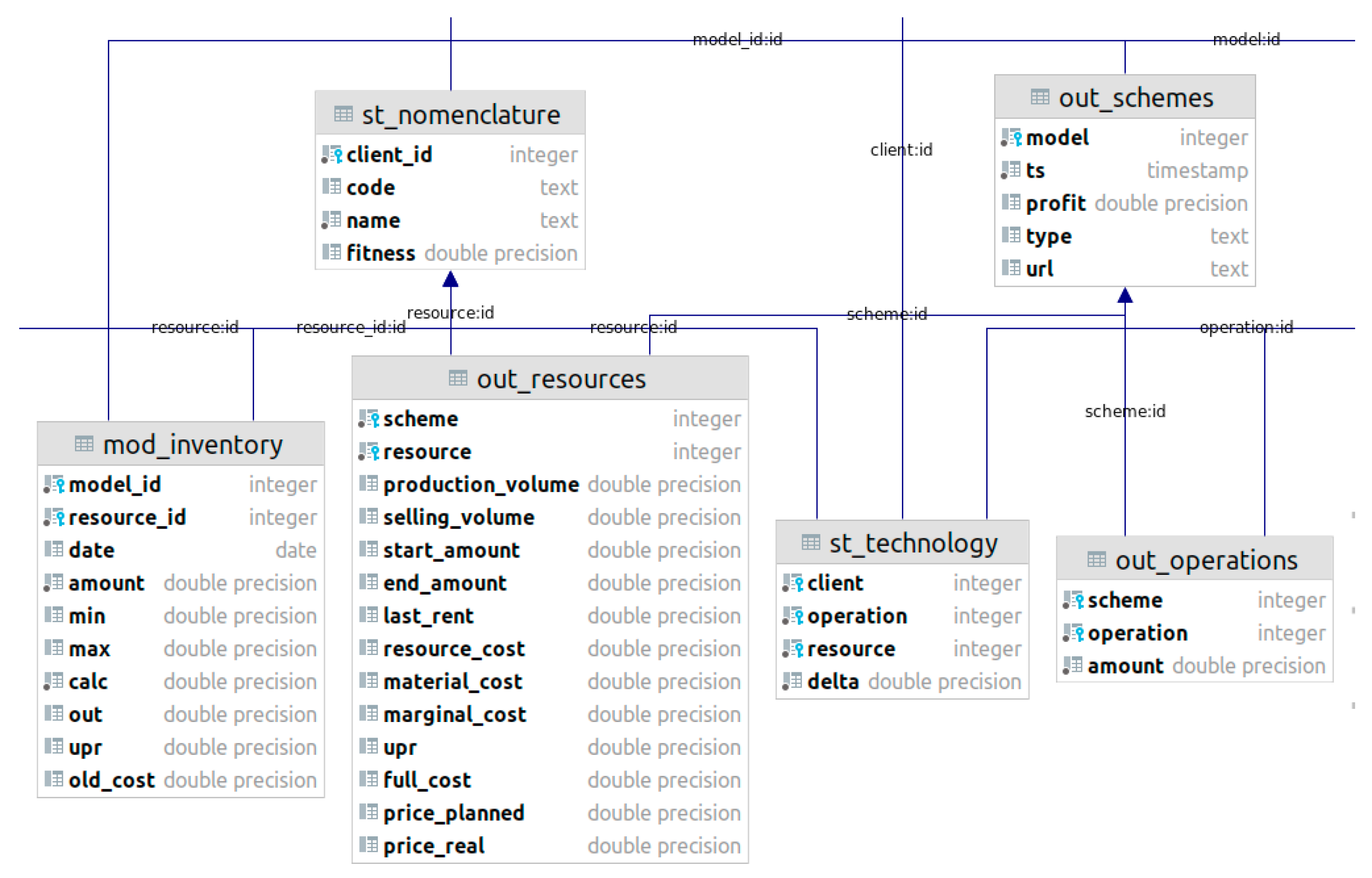
• Static tables, which are rarely changing tables of product nomenclature (st_nomenclature); a production flow chart (st_technology); a directory of enterprise suppliers (st_supply); a table of production operations with restrictions (st_operations); a directory of assortment groups of products, raw materials, and materials (st_categories); a directory organization (st_clients), which is necessary for the case when information about several manufacturing enterprises is stored in one database;
• Model calculation status information table (inf_statuses) to track the progress and production stages (inf_stages);
• Tables related to a specific reporting period of the simulation and subject to revision, in general, once a month—the table of models (mod_models), dynamically calculated restrictions on operations (mod_operations), and the initial state of production at the beginning of the reporting period (mod_inventory);
• Table containing the sales plan for each model in the corresponding reporting period, in_wishes;
• Tables containing the simulation results—production schemes (out_schemes), the volume of each production operation (out_operations), and information on the planned resource balance of the enterprise after the production scheme implementation (out_resources).

After loading the initial data, the information system performs the initial calculation of the production plan based on the fixed values of the sales plan. In most real production systems, alternative operations can exist, for example, different combinations of intermediate processing operations. This preliminary calculation considers the volumes of such alternative processes, on average, for the adequate calculation of the cost of production resources and the leading economic indicators—revenue and profit.

The primary purpose of the preliminary calculation is to give an approximate value of the planned profit of production with the exact implementation of the sales plan and determine the preliminary need for primary and auxiliary materials. In our demo example, when implementing a sales plan drawn up based on the recommendations of the subject area experts, we received a profit of the fundamental solution (production plan) at the level of RUR 67,902,234, 9.27% of production profitability in terms of net profit. This estimate is further used as a baseline profit level against which the best solution produced by the system during simulation is compared.

After calculating the basic solution, the simulation process starts. The variability of the generated production schemes is provided due to the presence of several factors. First, there are so-called alternative operations in any production scheme, a different combination of which can lead to the production of the same items of finished products or raw materials, but they have other economic efficiencies.

Secondly, in some cases, there is a choice of purchasing intermediate products or their production. In the same way, there is the possibility of selling intermediate production results or using them in further stages. Moreover, the economic efficiency of these options strongly depends on the market situation, namely, on the prices of raw materials and materials. Moreover, thirdly, production can obtain the effect of redistributing the volumes of finished products within assortment groups.

It is necessary to switch from point-to-point production volumes of finished products to interval ones to start the simulation. For this, the system operator must set the value of expanding the boundaries of the production volume of the product range. Empirically, it was found that the best results can be achieved by setting the minimum and maximum production volumes, respectively, 10% lower and 10% higher than the volume of the corresponding position in the sales forecast (this indicator can be varied). Thus, after expansion, we obtain an interval of possible production volume.

The actual stage of simulation is to generate production schemes within the specified constraints. For each production operation, technological restrictions are calculated, namely, the minimum and maximum volumes. These interval limits take into account the following factors:

• For the direct production of finished products, the restrictions correspond to interval estimates of the production volume of the corresponding name of the finished products;
• The operation should not produce more than the static constraints of the process;
• The operation must produce each resource, at least in the quantity required to produce the finished product in the required volume;
• The operation should not exceed the established labor costs and time intervals expressed in technological restrictions for this operation.

This system of conditions is justified by the requirements of compliance with the technical regulations of the enterprise; in general, it is not compatible.

If it detects that the specified restrictions are inconsistent, the system issues a message about the impossibility of generating production schemes under the specified conditions. The process of calculating static constraints into dynamic interval estimates for each operation is quite computationally expensive. However, it can be performed only once within the framework of the calculation of the primary solution. Then you can use the already calculated interval estimates, refining and narrowing them.

The optimal production scheme within the calculated dynamic interval estimates for each production operation consists of many production schemes’ sequential generation and calculation.

The process of calculating a specific production scheme (solution) includes the following steps:

• Calculation of dynamic and static constraints of production schemes;
• Generation of a production scheme within the established limits;
• Simulated application of the production scheme to the initial state;
• Calculation of the need for additional purchase and sale operations;
• Calculation of the value of the objective function of the production scheme;
• Calculation of economic indicators of the production scheme and data visualization.

Generation of a production scheme consists of generating a random vector, each value of which lies in the range of an interval estimate for each production operation related to the production of finished products; that is, to the last stage. It is essential that in the process of creating a prototype of the system, we concluded that it was inexpedient to generate a random volume of each production operation since setting accurate estimates for a given scheme for the production of finished products in many ways imposes more stringent restrictions on the intervals for performing other functions.

Thus, after the generation of the production scheme, the required volumes of the remaining production operations are calculated, depending on the need for resources produced by these operations. In this case, only the values that lie within the pre-calculated interval estimates were taken into account. Thus, all predetermined production limits were automatically taken into account.

The generation of production schemes can be carried out in several ways. As part of this study, we developed four methods for generating production schemes that are applicable in different use cases:

• Generation by average—a deterministic generator, when each production operation is performed in a volume corresponding to the average between the minimum and maximum volumes. This scheme is used to calculate the base solution and to test the program code for reproducibility;
• Random generation—a random value from a uniform distribution between the minimum and maximum values in the interval;
• Generation back through the production process—a variant of the previous generator. The volumes of finished products are randomly generated, and the volumes of previous operations are accordingly recalculated according to the demand for raw materials. This generator allows you to create more technologically correct circuits closer to real production and requiring fewer adjustments;
• Normalizing generator—a variant of the previous generator in which the generated values are additionally normalized to constant volumes of assortment groups. This generator allows you to vary the volume of products only within groups. The total produced volume remains constant, eliminating the impact on the potential profit of economies of scale.

After generating a production scheme, each scheme is calculated. The economic indicators of implementing such a scheme are calculated and balanced in the warehouses of finished products, raw materials, and materials. At this stage, the value of the objective function associated with each scheme is calculated. The main component of the objective function is the profit of the enterprise, which will be obtained when implementing this production scheme.

After generating and calculating a certain number of schemes (about the estimated number below), they are selected according to the value of the objective function, and several are chosen that are most optimal for manual verification by the enterprise management. At this stage, it is possible to adjust the schemes and accept the selected scheme in the form of the planned budget of the enterprise for the next reporting period.

3.4. Investigation of the Stability of Generation Results

As part of the proposed simulation model study, we carried out some numerical experiments to study the maximum found profit growth rate according to the optimal production scheme, depending on the generated schemes. Since the generation and calculation of simulation schemes is the most expensive process in computational complexity in the entire technique, it is crucial to know how many schemes are a reasonable compromise between maximizing profit and the time spent on generation.

For this, more than 40,000 simulations were produced. It turned out that the profit is distributed almost normally with the distribution center close to the profit of the base solution (see Figure 2). This coincides with the expected effect that approximately equivalent circuits will be better and worse than the base solution.

The profit of the base solution was RUR 64,902,234, which, strictly speaking, lies to the right of the centroid of the histogram distribution above. It was also justified because the sales plan on which the baseline solution was established was based on recommendations from subject matter experts, which positively affected its economic characteristics.

Next, we analyzed how the maximum found profit grows with an increase in the number of solutions. Since the generated circuits are entirely independent of each other, there was no need to run the simulation several times and average the results to improve robustness. It was enough to select the required number of simulations from one sufficiently large run. The results of this analysis are presented in

Table 3. Financial indicators of the demo case depending on the number of simulations performed.

Parameter	Absolute Value, RUR	Percentage of Revenue	Growth
Revenue	700,000,000.00
Base solution’s profit	64,902,234.00	9.27%
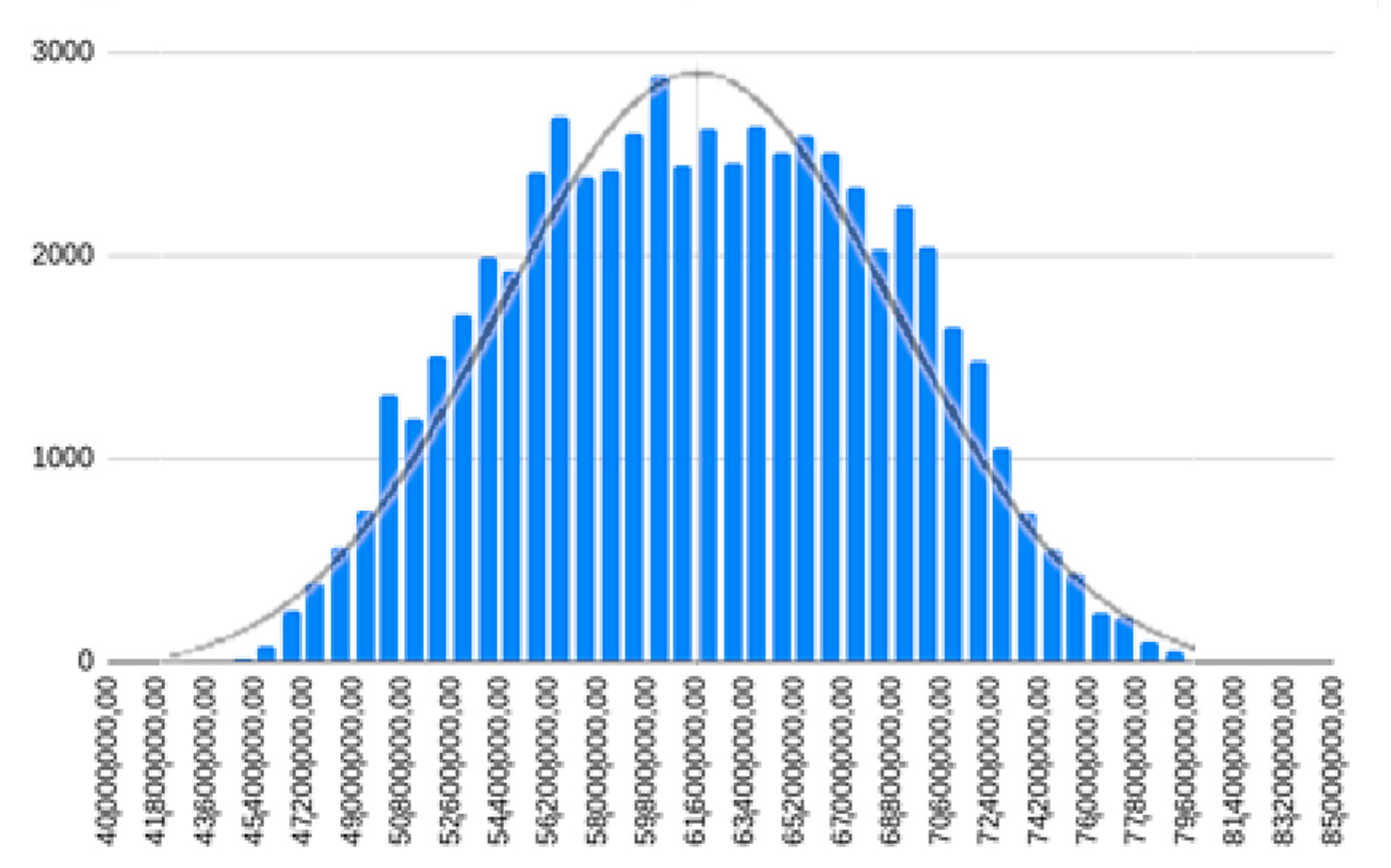
Maximum profit after 1000 simulations	78,856,870.00	11.27%	1.99%
Maximum profit after 5000 simulations	80,639,773.00	11.52%	2.25%
Benefit	15,737,539.00	1.24%

.

As can be seen from the table, after the first thousand simulations, the maximum found profit increased by more than 20%, a very significant economic effect. For example, if the profitability of the fundamental solution was 9.27%, then the best solution found by our algorithm achieved a profitability of 11.52% (after 5000 simulations). It can also be seen that the difference between the maximum profit for 1000 decisions and 5000 was entirely negligible, indicating a rapid stabilization of the simulation model. Thus, it was concluded that it was not advisable to generate more than 5000 circuits. For most practical applications, 1000 simulations are sufficient.

The calculations were carried out on a computer running an Intel Core i5-8265U CPU @ 1.60 GHz to test the model. On this hardware, it took precisely 46 s to generate one production circuit. Thus, it took about 13 h to develop 1000 solutions. It should be noted that this task scales very well, and we observed an almost linear relationship between the generation time and the power of the central processor.

In addition, in the course of the approbation of the model, the dependence of the model’s effectiveness on the magnitude of the variation in the volumes of the product range was investigated. As mentioned above, we took the 10% variation as the working value. The generated values were within ±10% of the sales plan volume for each position of the assortment of finished products. It should be noted that taking into account the subsequent normalization; the effective variation was precisely half of the nominal value; that is, after the normalization of volumes, they varied within an average of ±5% of the initial value. However, to investigate the robustness of the model, the values obtained with the various values of 10%, 20%, and 40% were tested. It has been suggested that by increasing the variation, the algorithm will find more efficient production patterns at the expense of a more extensive search space.

As can be seen from the figure, the hypothesis put forward was refuted entirely. The maximum value of the profit depends very little on the magnitude of the variation. We can explain this because the ability to find more efficient production schemes is entirely offset by the rarity of these “successful” solutions in a much more rarefied space.

In practice, this means that, when applying the proposed methodology in actual production, it is unnecessary to use high variation index values. Instead, the recommended level of 10% is enough to achieve this information system’s optimal efficiency level.

4. Conclusions

Automation and acceleration of the calculation process and the search for optimal production schemes have a complex positive effect on the organization and performance of a manufacturing enterprise. According to our observation, this effect consists of several aspects. First of all, it enables finding a more efficient production plan than calculated by classical methods. Secondly, this approach can reduce the cost of manual labor of the planning or financial department of the enterprise and improve the efficiency and speed of decision making in the enterprise. Moreover, this stimulates streamlining corporate databases to implement a single data warehouse that serves as a source of objective truth in the enterprise.

The direct effect of using the proposed production simulation methodology was analyzed above. According to our estimates, based on the analysis of the numerical calculations, in general, such a system can increase the company’s profit from 0.5 to 1.5 percentage points relative to the company’s monthly revenue.

Most significant from the point of view of enterprise management may be the effect of a radical change in the decision-making paradigm in planning the monthly production budget. In consultation with domain experts, we found that a surprisingly large number of manufacturing plants use simplified methodologies to plan their manufacturing processes. In this regard, the calculation of economic indicators takes several person-days of labor. Therefore, in practice, the scenario method is used when in the form of a draft budget, two, less often three, options for a production scheme are fully calculated, then analyzed, and combined.

The developed system allows for the forecasting of budget options to substantiate the best management decisions and online cumulatively, for example, daily analyzing the parameters of sales volumes, revenue, and profit, depending on the specific sales volumes, prices, etc., which are possible reasons for deviations from the budget.

References

- Pratap, S.; Jauhar, S.K.; Paul, S.K.; Zhou, F. Stochastic optimization approach for green routing and planning in perishable food production. J. Clean. Prod. 2022, 333, 130063. [Google Scholar] [CrossRef]
- Azzaro-Pantel, C.; Madoumier, M.; Gésan-Guiziou, G. Development of an ecodesign framework for food manufacturing including process flowsheeting and multiple-criteria decision-making: Application to milk evaporation. Food Bioprod. Processing 2022, 131, 40–59. [Google Scholar] [CrossRef]
- Zhang, L.; Deng, Q.; Zhao, Y.; Fan, Q.; Liu, X.; Gong, G. Joint optimization of demand-side operational utility and manufacture-side energy consumption in a distributed parallel machine environment. Comput. Ind. Eng. 2022, 164, 107863. [Google Scholar] [CrossRef]
- Fahimnia, B.; Farahani, R.Z.; Marian, R.; Luong, L. A review and critique on integrated production-distribution planning models and techniques. J. Manuf. Syst. 2013, 32, 1–19. [Google Scholar] [CrossRef]
- De Sampaio, R.J.B.; Wollmann, R.R.G.; Vieira, P.F.G. A flexible production planning for rolling-horizons. Int. J. Prod. Econ. 2017, 190, 31–36. [Google Scholar] [CrossRef]
- Bozek, P.; Nikitin, Y.; Bezak, P.; Fedorko, G.; Fabian, M. Increasing the production system productivity using inertial navigation. Manuf. Technol. 2015, 15, 274–278. [Google Scholar]
- Kongchuenjai, J.; Prombanpong, S. An integer programming approach for process planning for mixed-model parts manufacturing on a CNC machining center. Adv. Prod. Eng. Manag. 2017, 12, 274–284. [Google Scholar] [CrossRef] [Green Version]
- Chou, Y.-C.; Hong, L.-H. A methodology for product mix planning in semiconductor foundry manufacturing. IEEE Trans. Semicond. Manuf. 2000, 13, 278–285. [Google Scholar] [CrossRef]
- Panda, A.; Jurko, J.; Pandova, I. Monitoring and Evaluation of Production Processes, 1st ed.; Springer: Cham, Switzerland, 2016. [Google Scholar]
- Chung, S.-H.; Lee, A.H.I.; Pearn, W.L. Product mix optimization for semiconductor manufacturing based on AHP and ANP analysis. Int. J. Adv. Manuf. Technol. 2005, 25, 1144–1156. [Google Scholar] [CrossRef]
- Tanhaei, F.; Nahavandi, N. Algorithm for solving product mix problem in two-constraint resources environment. Int. J. Adv. Manuf. Technol. 2013, 64, 1161–1167. [Google Scholar] [CrossRef]
- Aryanezhad, M.B.; Komijan, A.R. An improved algorithm for optimizing product mix under the theory of constraints. Int. J. Prod. Res. 2004, 42, 4221–4233. [Google Scholar] [CrossRef]
- Amin Badri, S.; Ghazanfari, M.; Shahanaghi, K. A multi-criteria decision-making approach to solve the product mix problem with interval parameters based on the theory of constraints. Int. J. Adv. Manuf. Technol. 2014, 70, 1073–1080. [Google Scholar] [CrossRef]
- Escudero, L.F.; Kamesam, P.V.; King, A.J.; Wets, R.J.-B. Production planning via scenario modelling. Ann. Oper. Res. 1993, 43, 309–335. [Google Scholar] [CrossRef]
- Smith, J.S. Survey on the use of simulation for manufacturing system design and operation. J. Manuf. Syst. 2003, 22, 157–171. [Google Scholar] [CrossRef]
- Ponsignon, T.; Mönch, L. Simulation-based performance assessment of master planning approaches in semiconductor manufacturing. Omega 2014, 46, 21–35. [Google Scholar] [CrossRef] [Green Version]
- Straka, M.; Malindzakova, M.; Trebuna, P.; Rosova, A.; Pekarcikova, M.; Fill, M. Application of EXTENDSIM for improvement of production logistics’ efficiency. Int. J. Simul. Model. 2017, 16, 422–434. [Google Scholar] [CrossRef]
- Chen, Y.X. Integrated optimization model for production planning and scheduling with logistics constraints. Int. J. Simul. Model. 2016, 15, 711–720. [Google Scholar] [CrossRef]
- Melouk, S.H.; Freeman, N.K.; Miller, D.; Dunning, M. Simulation optimization-based decision support tool for steel manufacturing. Int. J. Prod. Econ. 2013, 141, 269–276. [Google Scholar] [CrossRef]
- Güçdemir, H.; Selim, H. Customer centric production planning and control in job shops: A simulation optimization approach. J. Manuf. Syst. 2017, 43, 100–116. [Google Scholar] [CrossRef]
- Ankenman, B.E.; Bekki, J.M.; Fowler, J.; Mackulak, G.T.; Nelson, B.L.; Yang, F. Simulation in production planning: An overview with emphasis on recent developments in cycle time estimation. In Planning Production and Inventories in the Extended Enterprise, 1st ed.; Kempf, K., Keskinocak, P., Uzsoy, R., Eds.; Springer: New York, NY, USA, 2011; pp. 565–591. [Google Scholar]
- Vasant, P.; Barsoum, N. Hybrid pattern search and simulated annealing for fuzzy production planning problems. Comput. Math. Appl. 2010, 60, 1058–1067. [Google Scholar] [CrossRef] [Green Version]
- Nazari-Shirkouhi, S.; Eivazy, H.; Ghodsi, R.; Rezaie, K.; Atashpaz-Gargari, E. Solving the integrated product mix-outsourcing problem using the Imperialist Competitive Algorithm. Expert Syst. Appl. 2010, 37, 7615–7626. [Google Scholar] [CrossRef]
- Fedorko, G.; Rosova, A.; Molnar, V. The Application of computer simulation in solving traffic problems in the urban traffic management in Slovakia. Theor. Empir. Res. Urban Manag. 2014, 9, 5–17. [Google Scholar]
- Saderova, J.; Kacmary, P. The simulation model as a tool for the design of number of storage locations in production buffer store. Acta Montan. Slovaca 2013, 18, 33–39. [Google Scholar]
- Homem-De-Mello, T.; Bayraksan, G. Monte Carlo sampling-based methods for stochastic optimization. Surv. Oper. Res. Manag. Sci. 2014, 19, 56–85. [Google Scholar] [CrossRef]
- Cai, T.; Wang, S.; Xu, Q. Monte Carlo optimization for site selection of new chemical plants. J. Environ. Manag. 2015, 163, 28–38. [Google Scholar] [CrossRef] [PubMed]
- Janekova, J.; Kovac, J.; Onofrejova, D. Application of modelling and simulation in the selection of production lines. Appl. Mech. Mater. 2015, 816, 574–578. [Google Scholar] [CrossRef]
- Janekova, J.; Fabianová, J.; Izarikova, G.; Onofrejová, D.; Kovač, J. Product Mix Optimization Based on Monte Carlo Simulation: A Case Study. Int. J. Simul. Model. 2018, 17, 295–307. [Google Scholar] [CrossRef]
- Li, M.; Yang, F.; Uzsoy, R.; Xu, J. A metamodel-based Monte Carlo simulation approach for responsive production planning of manufacturing systems. J. Manuf. Syst. 2016, 38, 114–133. [Google Scholar] [CrossRef] [Green Version]
- Cheng, G.; Li, L. Joint optimization of production, quality control and maintenance for serial-parallel multistage production systems. Reliab. Eng. Syst. Saf. 2020, 204, 107146. [Google Scholar] [CrossRef]
- Faaland, B.; Mark, M.K.; Thomas, S. A fixed rate production problem with Poisson demand and lost sales penalties. Prod. Oper. Manag. 2019, 28, 516–534. [Google Scholar] [CrossRef]
- Cheng, G.Q.; Zhou, B.H.; Li, L. Joint optimization of production rate and preventive maintenance in machining systems. Int. J. Prod. Res. 2016, 54, 6378–6394. [Google Scholar] [CrossRef]
- Chernyakova, I.S. Primenenie metodov imitatsionnogo modelirovaniya v ramkakh pravleniya finansovoy ustoychivostyu predpriyatiy myasopererabatyvayuschey otrasli application of the methods of imitation modeling within the framework of the management of the financial stability of the enterprises of meat processing industry. Ekon. Predprin. Pravo 2019, 9, 81–92. [Google Scholar]