Abstract
Industry 4.0 is characterized by the availability of sensors to operate the so-called intelligent factory. Predictive maintenance, in particular, failure prediction, is an important issue to cut the costs associated with production breaks. We studied more than 40 publications on predictive maintenance. We point out that they focus on various machine learning algorithms rather than on the selection of suitable datasets. In fact, most publications consider a single, usually non-public, benchmark. More benchmarks are needed to design and test the generality of the proposed approaches. This paper is the first to define the requirements on these benchmarks. It highlights that there are only two benchmarks that can be used for supervised learning among the six publicly available ones we found in the literature. We also illustrate how such a benchmark can be used with deep learning to successfully train and evaluate a failure prediction model. We raise several perspectives for research.
1. Introduction
Industry 4.0 has received growing attention in the last decade [1,2]. In 2013, the German government considered the Industry 4.0 project as a major effort to establish leadership in the industry. It was identified as one of the “10 Projects for the Future” in the High Technology Action Plan for 2020. In 2014, the Chinese government declared, as part of a 10-year national plan, “to make China the manufacturing workshop of the world and a global manufacturing power”, and is counting on the upgrade of its industry globally. In 2017, [3] noticed a continuous increase in the number of publications in the field of intelligent manufacturing from 2005 to 2016. The latest numbers of publications indexed on the Web of Science show a sharp increase in the number of publications since 2015, cf. Figure 1. This figure plots the number of publications on “intelligent manufacturing (all fields)” counted per year.
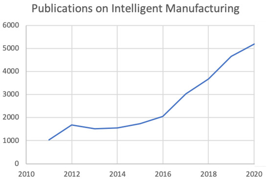
Figure 1.
Number of publications on “intelligent manufacturing (all fields)” counted on Web Of Science per year.
Industry 4.0 involves several technologies from different disciplines, such as Internet of Things, cloud computing, big data analysis, and artificial intelligence. In this work, we focus on machine failure prediction in Industry 4.0. Indeed, the success of factories depends closely on the reliability and quality of their machines and products. Unexpected machine breakdowns in production processes lead to high maintenance costs and production delays [4]. Therefore, understanding and predicting critical situations before they occur can be a valuable way of avoiding unexpected breakdowns and saving costs associated with failure. Thanks to the emerging technologies mentioned above, equipment in industrial production lines is increasingly connected and therefore, produces large volumes of data. These data can be analyzed and transformed into knowledge to enable decision makers to better manage maintenance.
Maintenance management approaches can be grouped into three main categories with different levels of complexity and effectiveness [5]:
- Reactive maintenance (also called run to failure): It is the simplest and least effective approach. Maintenance is performed only after failure has occurred, resulting in much greater intervention time and equipment downtime than that associated with planned corrective actions;
- Preventive maintenance: Here, maintenance actions are carried out according to a pre-established schedule, based on time or process iterations. With this approach, failures are usually avoided, but unnecessary corrective actions are often performed, leading to inefficient use of resources and increased operating costs;
- Predictive maintenance: In this approach, maintenance is carried out based on an estimate of the condition of a piece of equipment [6]. Predictive maintenance makes it possible, thanks to predictive tools based on historical data, to detect upcoming anomalies in advance and to perform maintenance in good time before a failure occurs.
In the field of predictive maintenance, our work focuses on the prediction of failures. We prefer the term “failure prediction” to make it clear that we want to predict, at a given moment, that a failure will occur in the future. We avoid the term “anomaly detection” because “detection” covers cases where one wants to find out at an instant that there is an anomaly already in progress at that instant, and “anomaly” refers to anything unusual and far broader than failures that can be prevented by maintenance. For example, the Kaggle Challenge on predicting production line performance [7] was initially formulated as an anomaly detection problem, as we will see in Section 4.4.
The prediction of failures explicitly takes into account the fact that the data are sequential, ordered in time. There are many challenges, including the following:
- The mass of data: the sensors automatically generate an amount of data that quickly reaches the order of a GB;
- Imbalanced data: failures are much less common than normal cases;
- The variety of the data: we often have to learn with few copies of the same machine, or even of the same family (but of different powers, for example).
These challenges are not specific to sequential data. However, they are almost always present, and more pronounced than when looking at other domains, especially without temporal data. Existing algorithms have to be improved or new algorithms have to be designed. Those algorithms have to be evaluated on various benchmarks in order to demonstrate their effectiveness on a range of applications.
This paper focuses on the identification of suitable benchmarks. To the best of our knowledge, it is the first paper dedicated to the identification of benchmarks for the prediction of failures in Industry 4.0. Our contributions are as follows:
- Browse the state of the art and point out that most published works on failure predictions considered their own private datasets;
- List explicitly the requirements on benchmarks to be used to train or evaluate a failure prediction model;
- Analyze six public benchmarks and highlight which ones are suitable and why the others are not;
- Illustrate the use of such benchmarks to train and evaluate a deep learning approach to predict the remaining useful life of a turbo-reactor.
This paper is organized as follows: Section 2 presents a comprehensive mapping of the work being done in Industry 4.0. Section 3 establishes the characteristics that datasets must meet in order to train and test algorithms to predict failures. Section 4 gives examples of good datasets and also counterexamples. Section 5 shows an example of using deep learning to predict the remaining useful life of a turbo-reactor. Section 6 concludes and lists some research perspectives.
2. Literature Review
Many works are published on the subject of Industry 4.0. A few papers give an overview of the field. We already referred to [3] for pointing out the increasing interest in intelligent manufacturing. They also study the positions of main industrial countries about Industry 4.0. In [4], the authors analyze the environment of Industry 4.0 and present the different technologies and systems that are used in this field. Ref. [8] proposes a conceptual framework of intelligent manufacturing systems for Industry 4.0 and presents several demonstrative scenarios, using key technologies such as IoT (Internet of Things), CPS (cyber–physical systems), and big data analytics. The security of those systems is an issue addressed in such projects as [9].
Other publications focus on techniques and applications. Among them, we find many machine leaning techniques. Ref. [10] focuses on cost-sensitive learning. An industrial application is studied but the data are not freely available and the experiments are completed by 25 public benchmarks outside industrial processes. Refs. [11,12] considers logical data analysis (LDA) methods. Ref. [11] presents a new methodology for predicting multiple failure modes on rotating machines. The proposed methodology merges a machine learning approach and a pattern recognition approach (LDA). The proposed methodology is validated using vibration data collected on bearing test stands. Ref. [12] proposes a technique called logical analysis of survival curves (LASC) to learn the degradation process and to predict the failure time of any physical asset. Similar to [11], the authors use machine learning and logical data analysis techniques to exploit instantaneous knowledge of the failure state of the physical asset being investigated. This method has been tested on data collected from sensors mounted on cutting tools.
Several deep learning techniques are used in the intelligent manufacturing context: deep neural networks [13], deep convolutional neural network [14], fuzzy neural networks [15], and wavelet neural network [16]. In [13], the authors use deep neural networks for failure prediction of rotating machines. Since it is generally difficult to obtain accurately labeled data in real industries, the authors propose data augmentation techniques to artificially create additional valid samples for model training. In [14], the authors propose a new method for predicting tool wear based on deep convolutional neural networks (DCNN). The performance of the method is validated on tool datasets from CNC (computer numerical control) machines running dry until failure. In [15], the authors propose multi-layer neural networks based on fuzzy rules to predict tool life; the method is validated on datasets collected from tools used in a dry milling operation. In [16], the authors investigate the application of a special variant of artificial neural networks (ANN), in particular the wavelet neural network (WNN), for monitoring tool wear in CNC high-speed steel end milling processes.
Other approaches, such as Markov processes, association rules mining, SVM, random forests and XGBoost, are used together with similarity-based residual life prediction techniques or fuzzy inference techniques. In [17], the authors consider the application of a state space model for predicting the remaining useful life of a turbo-fan engine. In [18], the authors propose a technique to improve the prediction of the remaining useful life based on similarity. The authors perform an experiment on the remaining useful life of gyroscopes to validate the approach. In [19], the authors propose a failure prediction method based on multifactorial fuzzy time series and a cloud model. In [20], the authors use random forests for the predictive maintenance of a cutting machine. Ref. [21] uses random forests and XGBoost in a predictive maintenance system for production lines. In [22], the authors propose an innovative maintenance policy. It aims both at predicting component failures by extracting association rules and at determining the optimal set of components to be repaired in order to improve the overall reliability of the factory, within time and budget constraints. An experimental campaign is conducted on a real case study of an oil refinery plant.
Techniques of imagery and learning methods are also used together. In [23], the authors present a new approach for classifying tool wear, based on signal imaging and deep learning. By combining these two techniques, the approach allows to work directly with the raw data, avoiding the use of statistical preprocessing or filtering methods. In [24], the authors present a methodology to automatically detect defective crankshafts. The proposed procedure is based on digital image analysis techniques to extract a set of representative features from crankshaft images. Supervised statistical classification techniques are used to classify the images, according to whether or not they are defective.
To summarize, the existing publications on failure prediction in Industry 4.0 have focused on its applications and on the learning algorithms but no publication has focused on the benchmarks available for failure prediction in Industry 4.0, as done in this work. In fact, each publication considers one or a few datasets. Most of the time, those datasets are private. However, public datasets are useful to compare to, or at least reproduce, existing approaches. The availability of distinct datasets helps to design generic approaches. In all the works cited previously, we found only two benchmarks that are publicly available and suitable for failure prediction.
3. Required Characteristics of a Benchmark for Failure Prediction
Let us first identify the characteristics that a benchmark should satisfy to be used to train and test an algorithm for failure prediction.
In this paper, we do not differentiate between data flows, sequential data and temporal data. We assume that the data arrive continuously. This is emulated when we work with existing datasets. The data have timestamps that allows us to order the data into sequential data. We do not impose a constant frequency of data arrival. The order, or rather the sequence, of the data is the important characteristic. Some algorithms are designed to learn from sequences, e.g., deep learning approaches, such as LSTM [25,26,27]. Otherwise, the use of a sliding window of fixed width allows to transform a sequence into classical attribute–value data and thus, to use algorithms that are not dedicated to sequences initially, hence the whole set of algorithms available in the usual learning libraries.
In machine learning, it is important to identify the individual (or, in a complementary way, the population) on which one is generalizing. In the case of sequential data, we consider that each moment corresponds to an individual. For example, if we are interested in a machine whose breakdowns we want to predict, we collect data with a certain frequency. Every moment that data are collected is an individual. This is a typical setting and it is used in many works, e.g., [13,14,15,16].
Let us emphasize that making predictions at every timepoint is very different from the so-called time series classification (TSC). Indeed in TSC, the learning task is the classification of an entire series [28,29,30,31], i.e., to assign a single label to the whole sequence. Our aim is to assign a class value to each individual of the sequence.
We are in the context of supervised learning, where a label is associated to each individual. Indeed, the goal is to learn a model that predicts the value of that label for a new individual, which is another moment in our case. For example, we need to know at each instant if it is less than 3 days before the next breakdown. In this example, we assume that 3 days is the reasonable duration to organize maintenance. We use classification techniques if the label is qualitative/categorical or regression techniques if the label is quantitative/numerical. Since we are interested in predicting failures, we assume that data collection stops when a failure occurs. Indeed, it can be assumed that data collection resumes when the failure has been corrected, and this constitutes a new sequence. Thus, each learning sequence ends with a failure. In this case, if we adopt the point of view of classification, we can define the label as a Boolean indicating whether the failure will occur in less than a given threshold, this threshold corresponding to the time needed to plan maintenance and reorganize the production. Alternatively, instead of classifying by setting a threshold, one can take the regression viewpoint and define the label to be predicted as the time remaining before the failure, known as the remaining useful life (RUL), e.g., [32].
The question of classifying only the last moment or each moment of a sequence raises the question of the link between the sequences that are used to learn the model and the sequences on which predictions are made, using this model. A special case is the case of a data flow, and thus, a single data sequence, the part of which is already seen can be used as training data to build a model that is applied to the data that follow. In many cases, there are several distinct sequences. The question is whether these sequences relate to the same machine as in the bearings dataset [33]. If the sequences relate to different machines, the differences may be of several kinds:
- There can be several physical exemplars of exactly the same model of machine;
- The machines can be of the same family but of different power ratings, for example;
- We can generalize to “similar” machines, i.e., comparable for learning and prediction, but possibly from different families.
In all cases, the construction and then application of a model requires finding a common, “comparable”, representation of the data, for example, by integrating the power, the model and the family of machines under consideration. Training and test data are said to be representative if the model learned from the training data can be applied, with relevance, to the test data. In [34], the authors notice that many datasets are provided as separate training and test sets, but the frequencies of the classes are very different. These training and test sets, therefore, do not come from the same population and should not be compared.
In conclusion, we recommend that a dataset for supervised learning consists of sequences as follows:
- All are comparable to each other, i.e., having the same representation, including a description of their similarities and differences, making it possible to learn a model from any subset of these sequences and to be able to apply this model to the remaining sequences;
- Each sequence ends with a failure/anomaly, making it possible to determine the value of the label for each instance of the sequence.
4. Analysis of the Publicly Available Benchmarks
In all the works cited in Section 2, we found only two benchmarks that are publicly available. These benchmarks are the bearing datasets [32,33,35,36,37,38] and the TurboFan datasets [39,40]. In this section, we analyze them plus three additional benchmarks dealing with fault prediction available on the internet. We describe each one and check whether it meets the characteristics required above.
4.1. Secom
The SECOM dataset [41] concerns a semiconductor manufacturing process. There are 591 attributes for a dataset with 1567 examples. Only 104 examples end with a failure. The remaining 1463 “examples” cannot be used in a supervised approach because they cannot be assigned a label since it is not known when the failure will occur (in fact, when the failure occurred for the training and test data). Moreover, these sequences are short: 18 timestamps on average, and even 3 for the shortest one. This does not leave time to organize maintenance, and therefore, it is not relevant to try to predict failure in this context.
4.2. Li-Ion Battery Aging
The lithium–ion battery aging dataset [42] is intended to predict the remaining charge on the one hand, and the remaining lifetime (before the battery capacity has decreased by more than 30%) on the other hand. Each sequence consists of charge and discharge cycles. A total of 5 to 7 attributes are measured according to the current state of the cycle. However, only 4 batteries are tested. This provides too few examples on which to learn and test.
4.3. Bearings
This benchmark is about four bearings installed on a shaft [38]. There are three datasets. Each of them describes a test-to-failure experiment. So the remaining useful life (RUL) looks well defined. Vibrations were measured using accelerometers installed on the bearing housing for each bearing. The first difficulty is that 8 accelerometers were used in the first dataset, while only 4 accelerometers were used in the second and third datasets; this makes difficult to generalize among those datasets. Moreover, the failures concern different parts: bearings 3 and 4 for the first dataset, bearing 1 for the second dataset and bearing 3 for the third dataset. A second difficulty is whether it is possible to generalize from one bearing to another, knowing that their locations are different [33] (Figure 16). Finally there are too few failures—4 failures altogether in the three datasets—to train and test a predictive model.
4.4. The Challenges of the Bosch Dataset
The Bosch company offered a contest on Kaggle [43]. This contest concerns the prediction of the quality of the parts produced. The dataset is related to 1,184,687 products, described by 968 numerical values of the individual sensors and 1156 timestamps corresponding to the time of passage through the individual sensors. The data are not further detailed by the company. It is only known that there are 51 stations on a total of 4 production lines.
We can already notice the following:
- The proposed dataset is large (14.3 GB). Each operation on such a large amount of data is difficult;
- There are only 6879 faulty products, 0.58% of the products. Thus, the data are extremely unbalanced;
- Many values are missing. All the parts do not go through all the stations, as can be seen in Figure 2 which shows the number of parts going through each of the 51 stations, so the parts do not have values for the attributes of the stations they do not go through. We will come back to this difficulty.
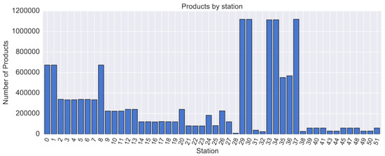 Figure 2. Products count passing through each station.
For these reasons, the proposed competition on Kaggle is difficult. However, the competition was not really a predictive maintenance problem. Indeed, the aim was to “predict” the quality of the part, described by the values measured during its production, i.e., once it is already produced. The values of the descriptors at time t are used to predict the class at this same time t. There is no prediction of the class from data collected before the part is produced. However, this is how one could avoid producing defective parts instead of observing their poor quality afterwards. A predictive maintenance goal involves predicting the production of a defective part well in advance of its production, sufficiently in advance to plan maintenance. In this context, the predictive maintenance would suggest to replace a worn tool before defective parts are produced.
We could use the timestamps to reconstruct the sequence in which the parts were produced and use this sequence to predict the quality of the next parts from the parts already produced. In addition, we assume that each time a part is defective, a correction is made on the production line and, therefore, each defective part indicates the end of a sequence, after which a new sequence starts. Hence, the parts could become the instance/individuals we work on. The number of defective parts would become the number of sequences. The ratio of the number of times that a part is defective does not change, and the same applies if a threshold is entered for the time before the defective part. On the other hand, if one wants to learn the remaining useful life (RUL), each instance/part in the sequence can be labeled by the number of parts between it and the end of the sequence.
The main difficulty comes from the “missing” values. To begin with, it should be noticed that the values of the attributes of the stations where the parts do not pass are not missing. They could be assigned an explicit value of “does not pass through this station”. Although all attributes are numerical and it is difficult to give a numerical value to “does not pass through this station”, this difficulty is manageable. The real difficulty is not knowing which station is faulty, and this is the real missing value. Since we guess that when faulty parts are produced, the fault is corrected in order to produce correct parts again, information about the station that caused the fault exists but is missing. Without this information, the actual value of the remaining useful life cannot be determined.
4.5. Hard Drives’ Lifetime
The backblaze website [44] provides quarterly statistics and data on the remaining useful life of its hard disks. On Figure 3, we can see that at the end of September 2019, the company collected data on 112,864 hard disks; 6078 have died and the remaining 106,786 disks that have not yet failed can be used neither for training nor for testing in a supervised approach.
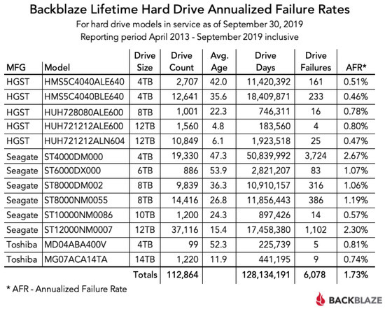
Figure 3.
Backblaze statistics in September 2019.
The disks come from four manufacturers and are of several models. If we want to use all of them for learning and testing, we must make sure that they all have the same descriptors and that the descriptors include the characteristics of the disks (manufacturer, model, capacity). Often, studies focus on the most common model [45,46,47,48]. There are 3724 copies of the Seagate ST4000DM000 model that have failed. This provides a consistent dataset, in which the disks are described by the same attributes. In fact, the data contain the date (since it is collected daily), the serial number and model of the disk, its capacity, a failure indicator, and 45 S.M.A.R.T. (self-monitoring, analysis and reporting technology) attributes with their raw and normalized values. Pre-processing is required to generate the sequences, with one file per serial number containing one line per date, since the data are provided by date with one line per serial number. Thus, the parts of this dataset that relate to failed disks which have the same descriptors can be used to train and test failure prediction models.
To summarize, this is the single benchmark that can be used to learn and evaluate models predicting failures of devices. The first four benchmarks did not satisfy the requirements to do so. Another positive example, satisfying those requirements, are presented in the next section.
5. Deep Learning on Turbofan
This section illustrates how a dataset satisfying the requirements identified in Section 3 can be used to predict the remaining service life and thus, for predictive maintenance. Our aim is to show how a dataset satisfying those requirements can be used properly to train and test a model. This experiment is intended neither to identify the best learner for this dataset, nor to evaluate the generality of the learning algorithm, but it focuses on the methodology, especially the collection of the right data.
Several simulation datasets on turbojet engine failure have been published by NASA [40,49]. We consider here the first dataset. A total of 100 sequences ending in failure are available. These sequences have lengths between 128 and 362, with an average of 206 instants. The values measured by 24 sensors are available at each instant. Each instant is labeled by the remaining useful life before the failure. This dataset satisfies the requirements listed in Section 3. Sequences are comparable to each other, as they have the same descriptors. Since the failure is known, each time point can be labeled with its remaining useful life. The lengths of the sequences are long enough to make predictions before the failures and, summed over the number of sequences, the population of all time points enable learning a complex model to predict the remaining useful life, for example, using deep learning.
Whereas [17] considered only 10 arbitrary test sequences, we use a random train–test split. The first 70 sequences are used to build a model, using LSTM [50]. The remaining 30 sequences are used as a test set. Figure 4 illustrates the used architecture. A fixed window length is defined and used to train the LSTM. A data normalization process is applied on all time series. In LSTM, the hyperbolic tangent is used as the activation of hidden neurons and the sigmoid for the gates. All features are used for training, due to the ability of LSTM to deal with non-relevant features. After trying other existing optimizers, an adamax optimizer is retained by experiments to fit the best model. Then, a dropout function is used between layers to prevent over-fitting. Finally, the last dense layer estimates the remaining useful life of the tested turbofan engine. The hyperparameters were set by preliminary experiments on a few sequences of the training set until the predictions successfully converged to a detection of the failure. In future work, cf. Section 6, we plan to favor underestimations over over-estimations, and to optimize the fitting near the duration needed to plan and perform the maintenance. Figure 5 contains a screenshot of the prediction software we implemented.
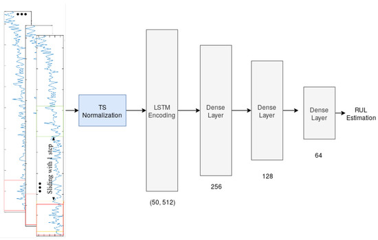
Figure 4.
LSTM architecture.
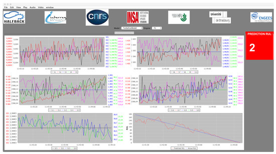
Figure 5.
Our remaining useful life prediction software.
The first 5 graphs, in reading order from left to right and from top to bottom, represent in real time the values of the 24 sensors. The graph at the bottom right represents the predictions made by our model (red curve) and the blue line is the actual remaining useful life. The screenshot is taken at the end of the program execution, i.e., with the predictions from the beginning to the end of the tested sequence.
6. Conclusions and Perspectives
We observed that in the literature on predictive maintenance in Industry 4.0, the same few benchmarks, namely battery aging, bearings and turbofan, are used. Indeed, few benchmarks are publicly available. There is a risk of over-fitting: designing learning techniques that perform well on those few datasets but poorly on other datasets. Our first recommendation is to experiment on as many datasets as possible, and also to make more datasets public, following the recent trend toward open science.
We examined a few other public datasets, namely Secom, Bosch challenge, and Backblaze Hard Drives; we showed that the first two datasets cannot be used to train models for predictive maintenance. The sequences in the Secom dataset are too short, 18 timestamps on average, to be representative of long-term maintenance. The Bosch challenge was not initially presented as sequential data: the aim was to predict the quality of a produced part from the sensors values collected during its production. Even though the sequence of parts produced is known, the faulty stations are not given, making impossible to learn to predict when a station will fail and require maintenance.
We highlighted the requirements on a dataset to learn a model to predict failures in manufacturing. The duration of the sequences should be greater than the time needed to plan a maintenance. The number of sequences should be sufficient to fit a model. The exact number depends both on the difficulty of the problem and on the expressiveness of the model, roughly its number of parameters. For example, learning a linear model requires fewer data, but it is relevant only if it performs well on the given problem. Hence, the right number of sequences can be checked by running experiments with the chosen learning technique and evaluating its performance, according to the state of the art, using a test–train split, and checking both the mean and the standard deviation [51]. For prediction, i.e., in a supervised approach, it is also necessary that the sequences end with a failure in order to be able to label each instance, with respect to the end of the sequence.
The Backblaze Hard Drive and the Turbofan benchmarks satisfy those requirements. We illustrated how a deep learning approach can be used to predict the remaining useful life on the Turbofan benchmark.
Test sequences, or training sequences, which do not end with a failure can be considered as long as each instance is labeled. This means that the end of the sequence is known, even though it is not provided. The test sequences in the Turbofan dataset are such a case: they end with an instance labeled by the time before the failure. Subsequent times are not provided. However, could we learn and test only with sequences ending before the end, for example 30 time units (days in the case of hard disks)? This would be acceptable if we know that 30 time units before the end is much too late to intervene to plan a maintenance, and that it is before 30 time units that our prediction is useful. This question is linked to a more general question about the range of time for which we want to predict the failure.
The range of time for which we want to predict the failure as accurately as possible is obviously around the duration needed to plan maintenance. Its exact value is indicated by experts, taking into account the time it takes to organize maintenance. From the point of view of machine learning, this means that one is particularly interested in a range of values. If we take the example of the predictions on the graph at the bottom right of Figure 5, we can imagine that the errors for values above 80 are less crucial than those for values closer to the failure. This is an aspect considered in machine learning, for example, when one privileges a part of the area under the ROC curve [52,53,54,55,56]; however, to the best of our knowledge, this has not been studied specifically for time series.
In supervised classification, a distinction is often made between false positives and false negatives. In regression also, an overestimation can be distinguished from an underestimation. Indeed, it is more serious to predict and therefore plan maintenance too late than too early. This aspect has been studied in the general case, for example, by [57], but not in the specific case of time series.
Author Contributions
Conceptualization, A.B., G.F. and N.L.; methodology, A.B. and N.L.; software, M.S.D. and S.A.M.; validation, M.S.D. and N.L.; formal analysis, M.S.D. and N.L.; investigation, M.S.D., S.A.M., A.B., G.F. and N.L.; resources, A.B.; data curation, M.S.D.; writing—original draft preparation, M.S.D., S.A.M. and N.L.; writing—review and editing, A.B. and G.F.; visualization, M.S.D.; supervision, N.L.; project administration, A.B. and N.L.; funding acquisition, A.B. All authors have read and agreed to the published version of the manuscript.
Funding
This research was funded by Upper Rhine INTERREG (European Regional Development Fund) and the Ministries for Research of Baden-Wurttemberg, Rheinland-Pfalz (Germany) and from the Grand Est French Region in the Upper Rhine Offensive Science HALFBACK project. The APC was funded by ICube Laboratory.
Conflicts of Interest
The authors declare no conflict of interest. The funders had no role in the design of the study; in the collection, analyses, or interpretation of data; in the writing of the manuscript; or in the decision to publish the results.
References
- Xu, L.D.; Xu, E.L.; Li, L. Industry 4.0: State of the art and future trends. Int. J. Prod. Res. 2018, 56, 2941–2962. [Google Scholar] [CrossRef] [Green Version]
- Usuga Cadavid, J.P.; Lamouri, S.; Grabot, B.; Pellerin, R.; Fortin, A. Machine learning applied in production planning and control: A state-of-the-art in the era of industry 4.0. J. Intell. Manuf. 2020, 31, 1531–1558. [Google Scholar] [CrossRef]
- Zhong, R.; Xu, X.; Klotz, E.; Newman, S. Intelligent Manufacturing in the Context of Industry 4.0: A Review. Engineering 2017, 3, 616–630. [Google Scholar] [CrossRef]
- Alcácer, V.; Cruz-Machado, V. Scanning the Industry 4.0: A Literature Review on Technologies for Manufacturing Systems. Eng. Sci. Technol. Int. J. 2019, 22, 899–919. [Google Scholar] [CrossRef]
- Susto, G.A.; Schirru, A.; Pampuri, S.; McLoone, S.; Beghi, A. Machine Learning for Predictive Maintenance: A Multiple Classifier Approach. IEEE Trans. Ind. Inform. 2015, 11, 812–820. [Google Scholar] [CrossRef] [Green Version]
- Krishnamurthy, L.; Adler, R.; Buonadonna, P.; Chhabra, J.; Flanigan, M.; Kushalnagar, N.; Nachman, L.; Yarvis, M. Design and Deployment of Industrial Sensor Networks: Experiences from a Semiconductor Plant and the North Sea. In Proceedings of the 3rd International Conference on Embedded Networked Sensor Systems, New York, NY, USA, 2–4 November 2015; ACM: New York, NY, USA, 2005; pp. 64–75. [Google Scholar] [CrossRef]
- Mangal, A.; Kumar, N. Using Big Data to Enhance the Bosch Production Line Performance: A Kaggle Challenge. arXiv 2017, arXiv:1701.00705. [Google Scholar]
- Zheng, P.; Wang, H.; Sang, Z.; Zhong, R.Y.; Liu, Y.; Liu, C.; Mubarok, K.; Yu, S.; Xu, X. Smart manufacturing systems for Industry 4.0: Conceptual framework, scenarios, and future perspectives. Front. Mech. Eng. 2018, 13, 137–150. [Google Scholar] [CrossRef]
- Karampidis, K.; Panagiotakis, S.; Vasilakis, M.; Markakis, E.K.; Papadourakis, G. Industrial CyberSecurity 4.0: Preparing the Operational Technicians for Industry 4.0. In Proceedings of the 2019 IEEE 24th International Workshop on Computer Aided Modeling and Design of Communication Links and Networks (CAMAD), Limassol, Cyprus, 11–13 September 2019; pp. 1–6. [Google Scholar] [CrossRef]
- Frumosu, F.D.; Khan, A.R.; Schiøler, H.; Kulahci, M.; Zaki, M.; Westermann-Rasmussen, P. Cost-sensitive learning classification strategy for predicting product failures. Expert Syst. Appl. 2020, 161, 113653. [Google Scholar] [CrossRef]
- Ragab, A.; Yacout, S.; Ouali, M.S.; Osman, H. Prognostics of multiple failure modes in rotating machinery using a pattern-based classifier and cumulative incidence functions. J. Intell. Manuf. 2019, 30, 255–274. [Google Scholar] [CrossRef]
- Elsheikh, A.; Yacout, S.; Ouali, M.S.; Shaban, Y. Failure time prediction using adaptive logical analysis of survival curves and multiple machining signals. J. Intell. Manuf. 2020, 31, 403–415. [Google Scholar] [CrossRef]
- Li, X.; Zhang, W.; Ding, Q.; Sun, J.Q. Intelligent rotating machinery fault diagnosis based on deep learning using data augmentation. J. Intell. Manuf. 2020, 31, 433–452. [Google Scholar] [CrossRef]
- Huang, Z.; Zhu, J.; Lei, J.; Li, X.; Tian, F. Tool wear predicting based on multi-domain feature fusion by deep convolutional neural network in milling operations. J. Intell. Manuf. 2019, 31, 953–966. [Google Scholar] [CrossRef]
- Li, X.; Lim, B.S.; Zhou, J.; Huang, S.G.; Phua, S.J.; Shaw, K.C.; Er, M.J. Fuzzy Neural Network Modelling for Tool Wear Estimation in Dry Milling Operation. In Proceedings of the Annual Conference of the Prognostics and Health Management Society, San Diego, CA, USA, 27 September–1 October 2009. [Google Scholar]
- Ong, P.; Lee, W.K.; Lau, R.J.H. Tool condition monitoring in CNC end milling using wavelet neural network based on machine vision. Int. J. Adv. Manuf. Technol. 2019, 104, 1369–1379. [Google Scholar] [CrossRef]
- Sun, J.; Zuo, H.; Wang, W.; Pecht, M.G. Application of a state space modeling technique to system prognostics based on a health index for condition-based maintenance. Mech. Syst. Signal Process. 2012, 28, 585–596. [Google Scholar] [CrossRef]
- Gu, M.; Chen, Y. Two improvements of similarity-based residual life prediction methods. J. Intell. Manuf. 2019, 30, 303–315. [Google Scholar] [CrossRef]
- Dong, L.; Wang, P.; Yan, F. Damage forecasting based on multi-factor fuzzy time series and cloud model. J. Intell. Manuf. 2019, 30, 521–538. [Google Scholar] [CrossRef]
- Paolanti, M.; Romeo, L.; Felicetti, A.; Mancini, A.; Frontoni, E.; Loncarski, J. Machine Learning approach for Predictive Maintenance in Industry 4.0. In Proceedings of the 14th IEEE/ASME International Conference on Mechatronic and Embedded Systems and Applications, MESA 2018, Oulu, Finland, 2–4 July 2018; pp. 1–6. [Google Scholar] [CrossRef]
- Ayvaz, S.; Alpay, K. Predictive maintenance system for production lines in manufacturing: A machine learning approach using IoT data in real-time. Expert Syst. Appl. 2021, 173, 114598. [Google Scholar] [CrossRef]
- Antomarioni, S.; Pisacane, O.; Potena, D.; Bevilacqua, M.; Ciarapica, F.E.; Diamantini, C. A predictive association rule-based maintenance policy to minimize the probability of breakages: Application to an oil refinery. Int. J. Adv. Manuf. Technol. 2019, 105, 1–15. [Google Scholar] [CrossRef]
- Martínez-Arellano, G.; Terrazas, G.; Ratchev, S. Tool wear classification using time series imaging and deep learning. Int. J. Adv. Manuf. Technol. 2019, 104, 3647–3662. [Google Scholar] [CrossRef] [Green Version]
- Remeseiro, B.; Tarrío-Saavedra, J.; Francisco-Fernández, M.; Penedo, M.G.; Naya, S.; Cao, R. Automatic detection of defective crankshafts by image analysis and supervised classification. Int. J. Adv. Manuf. Technol. 2019, 105, 3761–3777. [Google Scholar] [CrossRef]
- Ding, N.; Ma, H.; Gao, H.; Ma, Y.; Tan, G. Real-time anomaly detection based on long short-Term memory and Gaussian Mixture Model. Comput. Electr. Eng. 2019, 79, 106458. [Google Scholar] [CrossRef]
- Zhang, Y.; Xiong, R.; He, H.; Pecht, M.G. Long Short-Term Memory Recurrent Neural Network for Remaining Useful Life Prediction of Lithium-Ion Batteries. IEEE Trans. Veh. Technol. 2018, 67, 5695–5705. [Google Scholar] [CrossRef]
- Malhotra, P.; Vig, L.; Shroff, G.; Agarwal, P. Long Short Term Memory Networks for Anomaly Detection in Time Series. In Proceedings of the 23rd European Symposium on Artificial Neural Networks, ESANN 2015, Bruges, Belgium, 22–24 April 2015. [Google Scholar]
- Bondu, A.; Gay, D.; Lemaire, V.; Boullé, M.; Cervenka, E. FEARS: A Feature and Representation Selection approach for Time Series Classification. In Proceedings of The 11th Asian Conference on Machine Learning, ACML 2019, Nagoya, Japan, 17–19 November 2019; pp. 379–394. [Google Scholar]
- Appice, A.; Ceci, M.; Loglisci, C.; Manco, G.; Masciari, E.; Ras, Z.W. (Eds.) New Frontiers in Mining Complex Patterns—Second International Workshop, NFMCP 2013. In Proceedings of the Conjunction with ECML-PKDD 2013, Prague, Czech Republic, 27 September 2013; Lecture Notes in Computer Science. Springer: Berlin/Heidelberg, Germany, 2014; Volume 8399. [Google Scholar] [CrossRef]
- Grabocka, J.; Schilling, N.; Wistuba, M.; Schmidt-Thieme, L. Learning Time-series Shapelets. In Proceedings of the 20th ACM SIGKDD International Conference on Knowledge Discovery and Data Mining, New York, NY, USA, 24–27 August 2014; ACM: New York, NY, USA, 2014; pp. 392–401. [Google Scholar] [CrossRef]
- Ye, L.; Keogh, E. Time Series Shapelets: A New Primitive for Data Mining. In Proceedings of the 15th ACM SIGKDD International Conference on Knowledge Discovery and Data Mining, Paris, France, 28 June–1 July 2009; ACM: New York, NY, USA, 2009; pp. 947–956. [Google Scholar] [CrossRef]
- Teng, W.; Zhang, X.; Liu, Y.; Kusiak, A.; Ma, Z. Prognosis of the Remaining Useful Life of Bearings in a Wind Turbine Gearbox. Energies 2017, 10, 32. [Google Scholar] [CrossRef] [Green Version]
- Yoo, Y.; Baek, J.G. A Novel Image Feature for the Remaining Useful Lifetime Prediction of Bearings Based on Continuous Wavelet Transform and Convolutional Neural Network. Appl. Sci. 2018, 8, 1102. [Google Scholar] [CrossRef] [Green Version]
- Gay, D.; Lemaire, V. Should we Reload Time Series Classification Performance Evaluation ? (a position paper). arXiv 2019, arXiv:1903.03300. [Google Scholar]
- Qiu, H.; Lee, J.; Lin, J.; Yu, G. Wavelet filter-based weak signature detection method and its application on rolling element bearing prognostics. J. Sound Vib. 2006, 289, 1066–1090. [Google Scholar] [CrossRef]
- Duong, B.P.; Khan, S.A.; Shon, D.; Im, K.; Park, J.; Lim, D.S.; Jang, B.; Kim, J.M. A Reliable Health Indicator for Fault Prognosis of Bearings. Sensors 2018, 18, 3740. [Google Scholar] [CrossRef] [Green Version]
- Zhang, N.; Wu, L.; Wang, Z.; Guan, Y. Bearing Remaining Useful Life Prediction Based on Naive Bayes and Weibull Distributions. Entropy 2018, 20, 944. [Google Scholar] [CrossRef] [Green Version]
- Lee, J.; Qiu, H.; Yuand, G.; J, L. Bearing data set. In IMS, University of Cincinnati, NASA Ames Prognostics Data Repository, Rexnord Technical Services; NASA AMES, Moffett Field: Moffett Field, CA, USA, 2007. [Google Scholar]
- Khan, F.; Eker, O.F.; Khan, A.; Orfali, W. Adaptive Degradation Prognostic Reasoning by Particle Filter with a Neural Network Degradation Model for Turbofan Jet Engine. Data 2018, 3, 49. [Google Scholar] [CrossRef] [Green Version]
- Saxena, A.; Goebel, K.; Simon, D.; Eklund, N. Damage propagation modeling for aircraft engine run-to-failure simulation. In Proceedings of the 2008 International Conference on Prognostics and Health Management, Denver, CO, USA, 25 March 2008; pp. 1–9. [Google Scholar] [CrossRef]
- McCann, M.; Johnston, A. SECOM Data Set. 2008. Available online: https://archive.ics.uci.edu/ml/datasets/secom (accessed on 20 August 2021).
- Dashlink. Li-ion Battery Aging Datasets. 2010. Available online: https://data.nasa.gov/dataset/Li-ion-Battery-Aging-Datasets/uj5r-zjdb (accessed on 20 August 2021).
- Bosch. Kaggle: Bosch Production Line Performance. 2016. Available online: https://www.kaggle.com/c/bosch-production-line-performance (accessed on 20 August 2021).
- Backblaze. Hard Drive Data and Stats. 2019. Available online: https://www.backblaze.com/b2/hard-drive-test-data.html (accessed on 20 August 2021).
- Basak, S.; Sengupta, S.; Dubey, A. Mechanisms for Integrated Feature Normalization and Remaining Useful Life Estimation Using LSTMs Applied to Hard-Disks. In Proceedings of the 2019 IEEE International Conference on Smart Computing (SMARTCOMP), Washington, DC, USA, 12–15 June 2019; pp. 208–216. [Google Scholar] [CrossRef] [Green Version]
- Anantharaman, P.; Qiao, M.; Jadav, D. Large Scale Predictive Analytics for Hard Disk Remaining Useful Life Estimation. In Proceedings of the 2018 IEEE International Congress on Big Data (BigData Congress), Boston, MA, USA, 11–14 December 2018; pp. 251–254. [Google Scholar] [CrossRef]
- Basak, S.; Sengupta, S.; Dubey, A. A Data-driven Prognostic Architecture for Online Monitoring of Hard Disks Using Deep LSTM Networks. arXiv 2018, arXiv:1810.08985. [Google Scholar]
- Su, C.J.; Li, Y. Recurrent neural network based real-time failure detection of storage devices. Microsyst. Technol. 2019. [Google Scholar] [CrossRef]
- Dashlink. Turbofan Engine Degradation Simulation Data Set. 2010. Available online: https://data.nasa.gov/dataset/Turbofan-engine-degradation-simulation-data-set/vrks-gjie (accessed on 20 August 2021).
- Hochreiter, S.; Schmidhuber, J. Long Short-Term Memory. Neural Comput. 1997, 9, 1735–1780. [Google Scholar] [CrossRef] [PubMed]
- Witten, I.H.; Frank, E. Data Mining—Practical Machine Learning Tools and Techniques, 2nd ed.; The Morgan Kaufmann Series in Data Management Systems; Morgan Kaufmann: Burlington, MA, USA, 2005. [Google Scholar]
- Narasimhan, H.; Agarwal, S. A Structural SVM Based Approach for Optimizing Partial AUC. In Proceedings of the 30th International Conference on Machine Learning, ICML 2013, Atlanta, GA, USA, 16–21 June 2013; Volume 28, pp. 516–524. [Google Scholar]
- Narasimhan, H.; Agarwal, S. SVMpAUCtight: A new support vector method for optimizing partial AUC based on a tight convex upper bound. In Proceedings of the 19th ACM SIGKDD International Conference on Knowledge Discovery and Data Mining, KDD 2013, Chicago, IL, USA, 11–14 August 2013; Dhillon, I.S., Koren, Y., Ghani, R., Senator, T.E., Bradley, P., Parekh, R., He, J., Grossman, R.L., Uthurusamy, R., Eds.; ACM: New York, NY, USA, 2013; pp. 167–175. [Google Scholar] [CrossRef]
- Dodd, L.E.; Pepe, M.S. Partial AUC estimation and regression. Biometrics 2003, 59 3, 614–623. [Google Scholar] [CrossRef] [Green Version]
- Wang, Z.; Chang, Y.C.I. Marker selection via maximizing the partial area under the ROC curve of linear risk scores. Biostatistics 2011, 12, 369–385. [Google Scholar] [CrossRef] [PubMed] [Green Version]
- Ye, W.; Lin, Y.; Li, M.; Liu, Q.; Pan, D.Z. LithoROC: Lithography hotspot detection with explicit ROC optimization. In Proceedings of the 24th Annual International Conference on VLSI Design Automation, Tokyo, Japan, 21–24 January 2019. [Google Scholar]
- Hernández-Orallo, J. ROC curves for regression. Pattern Recognit. 2013, 46, 3395–3411. [Google Scholar] [CrossRef] [Green Version]
Publisher’s Note: MDPI stays neutral with regard to jurisdictional claims in published maps and institutional affiliations. |
© 2021 by the authors. Licensee MDPI, Basel, Switzerland. This article is an open access article distributed under the terms and conditions of the Creative Commons Attribution (CC BY) license (https://creativecommons.org/licenses/by/4.0/).