Hierarchical Transfer Learning for Cycle Time Forecasting for Semiconductor Wafer Lot under Different Work in Process Levels

Abstract

The accurate cycle time (CT) prediction of the wafer fabrication remains a tough task, as the system level of work in process (WIP) is fluctuant. Aiming to construct one unified CT forecasting model under dynamic WIP levels, this paper proposes a transfer learning method for finetuning the predicted neural network hierarchically. First, a two-dimensional (2D) convolutional neural network was constructed to predict the CT under a primary WIP level with the input of spatial-temporal characteristics by reorganizing the input parameters. Then, to predict the CT under another WIP level, a hierarchical optimization transfer learning strategy was designed to finetune the prediction model so as to improve the accuracy of the CT forecasting. The experimental results demonstrated that the hierarchically transfer learning approach outperforms the compared methods in the CT forecasting with the fluctuation of WIP levels.

1. Introduction

Wafer is an important raw material for manufacturing semiconductor devices [1], which has strict requirements for the schedule of order delivery. In the wafer fabrication process, wafer lot is the most basic production unit (generally including 16–25 silicon wafers [2]) in the semiconductor wafer fabrication system (SWFS), and the average time from release to product of a wafer lot is referred to as the wafer fabrication cycle time (CT) [3]. CT reflects the performance of the semiconductor wafer fabrication system and the maturity of wafer fabrication process, and it becomes an important optimization objective of SWFS [4].

Under the different make-to-stock strategies, the work in process (WIP; these items are either just being fabricated or waiting for further processing in a queue or a buffer storage) level in the workshop is changing. In accordance with the law of factory physics, Little’s Law, CT = WIP/TH (TH—throughput) [5], when the WIP quantity in a wafer fabrication plant changes, the influencing factors of the wafer fabrication CT, as well as the wafer fabrication CT, change accordingly. Based on the WIP level, the wafer CT shows different change rules [6]; therefore, the prediction of wafer fabrication CT at different WIP levels becomes a key issue.

Compared with the current job, the prediction of wafer fabrication CT at different WIP levels still faces the following challenges:

(1)

The semiconductor wafer fabrication system is extremely complex and huge (as shown in Figure 1a), and its complex production process of multiple re-entrant flow [7] leads to multiple factors of influencing CT, as well as a complex interaction relationship [8].

(2)

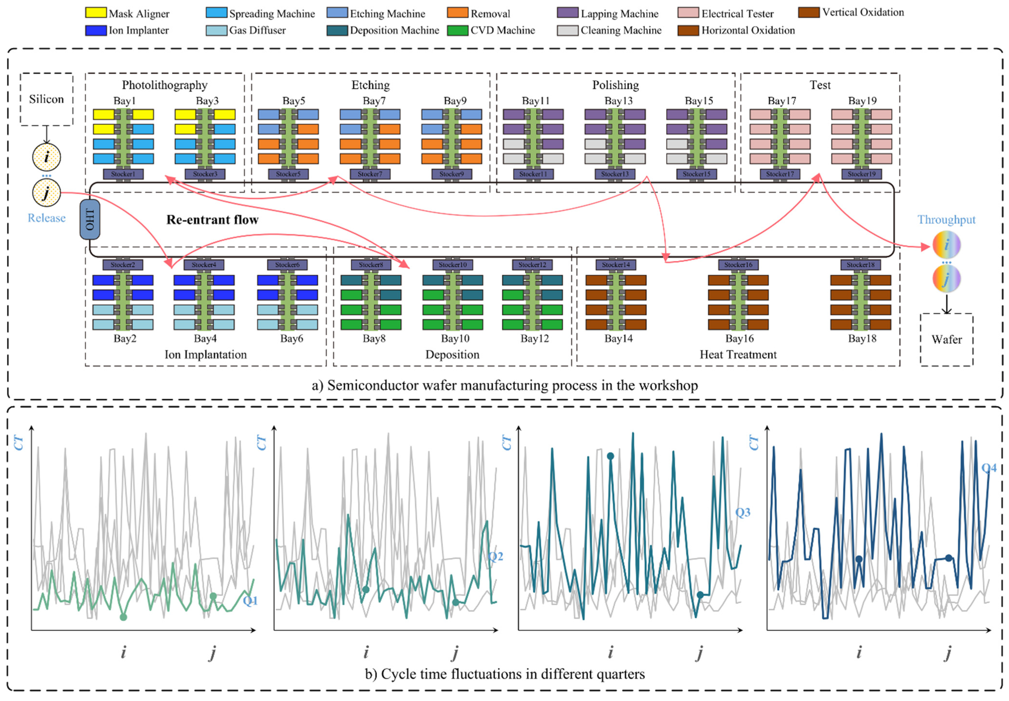
The wafer CT fluctuates (as shown in Figure 1b) after the make-to-stock strategies are changed; however, at this time, there are little data available to predict the wafer CT.

In terms of the CT prediction of such a complex manufacturing system, the two-dimensional (2D) convolutional neural network (CNN) was used in this present paper to extract the spatial-temporal characteristics of the reorganized characteristic parameters, build the wafer CT prediction model of a single WIP section, and achieve the wafer CT prediction of a single WIP section; then, the hierarchical optimization strategy was adopted to transfer and train the wafer CT prediction model at a new WIP level, and to achieve the wafer CT prediction of different WIP sections.

The structure of this paper is organized as follows. In Section 2, the current related research and existing problems are summarized. The transfer learning network of the hierarchical optimization is designed in Section 3. Section 4 conducts the example verification with wafer simulation data. Finally, the conclusions are summarized, and the direction of further research is pointed out in Section 5.

2. Related Works

The existing prediction methods for the wafer cycle time can be roughly divided into two categories, namely the model-based method and the data-driven method [9]. The model-based method refers to the prediction of the wafer fabrication CT using the simulation model or the basic mathematical model. Yang et al. [10] simulated the semiconductor manufacturing process by building a simulation model and obtained the predicted manufacturing CT from the simulation results. However, the semiconductor wafer fabrication system is quite huge and complex, and it takes a large amount of time and computing resources to complete the simulation. Therefore, it is difficult to build a high-precision and high-efficiency simulation model. Tai et al. [11] carried out a statistical analysis on the correlation between the wafer yield data and wafer CT data, and calculated the statistical indicators between them to predict the CT. Sha et al. [12] used parameter statistics to build the regression function of the wafer fabrication CT, and to predict the wafer CT. However, such a similar probability statistics function can only achieve a simple prediction of the average CT within a certain period of time, which is unable to predict the CT of the complex SWFS. On the basis of the classical queuing theory model, Roland et al. [13] predicted the CT in combination with multiple models. However, this method only took several simple processes into account, and it is equally difficult to predict the complex semiconductor wafer fabrication system. To sum up, model-based methods are difficult to predict the CT of the complex semiconductor wafer fabrication system because of its simplicity in structure and less processing data.

Compared with the model-based method, the data-driven method can analyze the fluctuation rules of the wafer CT using a mass of data, including process, queueing queue, and logistics system utilization ratio (see

Table 1. Influencing parameters of the cycle time.

Type	Parameters	Symbol
Wafer state parameters	Processing time for each process	$P{T}_1,\dots ,P{T}_n$
Equipment state parameters	Current use ratio of each device	$U_1,\dots ,U_m$
	Waiting queue length of each device	$Q_1,\dots ,Q_m$
Workshop state parameters	WIP quantity	$WIP$

), in the semiconductor wafer fabrication system. The common data-driven [14] methods include the decision-making tree [15,16], support vector machines (SVM) [17], and neural network [18,19]. Wu et al. [20] studied the scheduling problem of single-arm and double-arm robots by establishing the Petri Internet model, and predicted its processing cycle at the same time. Tirkel et al. [21] constructed a decision-making tree model by using the wafer circulation data to predict the wafer CT. Chang et al. [22] introduced the fuzzy rule to process the feature vector, and predicted the wafer CT through the case-based reasoning and neural network. Chen et al. [23] conducted in-depth research and analysis on the CT prediction successively, processed the characteristic vector by studying the self-organizing map, then used the fuzzy C-means to build the neural network, and achieved the prediction of wafer CT. Zhu et al. [24] proposed a method of support vector regression (SVR), designed the SVR model based on industrial big data, and achieved the prediction of wafer CT. These methods can build a complicated relationship between different characteristics and CT, but they depend on the human experience and have a poor generalization performance. In recent years, the deep neural network has shown an extraordinary performance in the processing and analysis of time series data. Wang et al. [25] proposed a bilateral long short-term memory (LSTM), considering wafer correlation and layer correlation, which achieved hidden state transmission to predict the CT accurately. Bai et al. [26] put forward a deep belief network (DBN) method. They firstly used the greedy algorithm to conduct the characteristic screening, and then the deep belief network to predict the quality of complex products. Wang et al. [27] constructed the DBN using the data collected from the workshop, and achieved the accurate prediction of the completion time of orders. The deep learning method can effectively analyze and extract the processing information from the influencing parameters. However, it usually requires a mass of data to train and optimize the prediction model. When the WIP level in the manufacturing system changes, there is the absence of extensive historical data to predict the wafer CT at a new WIP level.

The transfer learning, as an emerging learning paradigm, has become a hot research topic because it can transfer the knowledge learned from similar data to improve the model precision of a new target [28]. Such transfer can transmit the knowledge learned from sufficient data to a new environment in case of data deficiency [29], which is conducive to constructing the high-precision model under different environments. To achieve the prediction of wafer CT at different WIP levels, a transfer learning network based on hierarchical optimization was proposed in this paper. The two-dimensional (2D) convolutional neural network was used for the basic network model. Compared with the one-dimensional (1D) convolutional neural network, this present paper took the processing area characteristics of the multiple re-entrant flow wafer fabrication into account, used the 2D convolutional neural network to extract the spatial-temporal characteristics from the wafer fabrication data, and achieved the CT prediction at a single WIP level. Then, the transfer learning strategy based on the hierarchical optimization and the underlying structure sharing weights were used to extract the common characteristics of the manufacturing system at different WIP levels. After that, finetuning training was conducted on the high-level architecture to extract the specific characteristics of the manufacturing system at different WIP levels. Finally, the prediction of the wafer fabrication CT at different WIP levels was achieved.

3. Methods

This section elaborated the frame architecture of the prediction model of the wafer cycle time proposed. Firstly, the proposed hierarchical finetuning transfer network (HFTN) was described in detail; then, the training method of network was introduced.

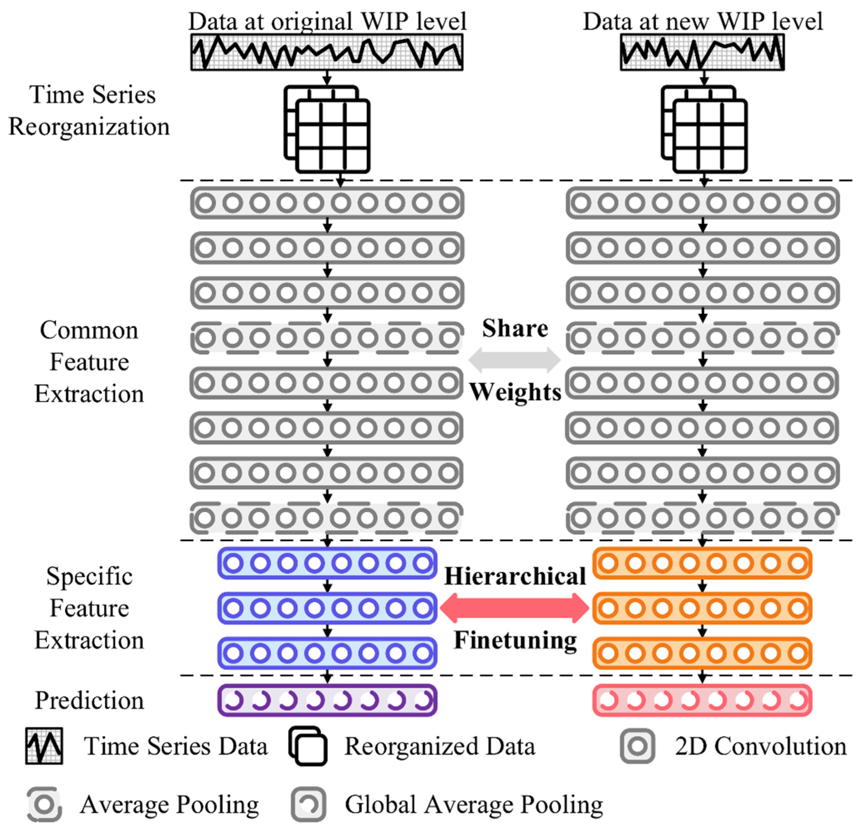
3.1. Architecture of Hierarchical Finetuning Transfer Network

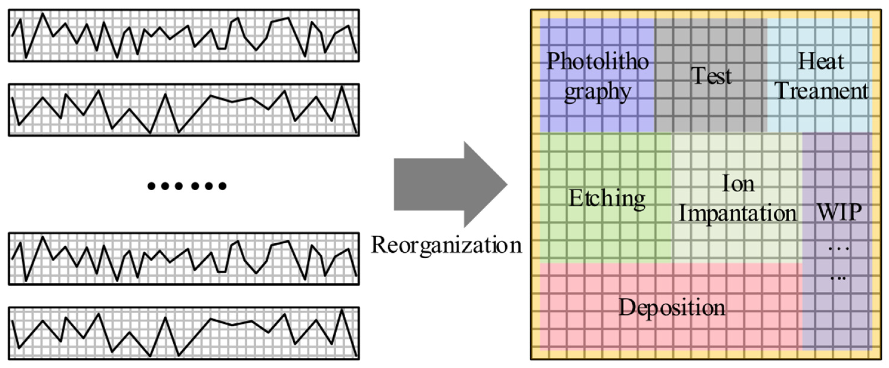
CNN [30] has shown an excellent performance in the time series prediction task, and the 2D CNN can effectively extract the time and space information from the reorganized time series data [31]. Therefore, 2D CNN was selected as the basic architecture of HFTN in this paper.

HFTN is composed of the following architectures: one input layer, nine 2D convolutional layers, two average pooling layers, and one global average pooling layer as the output layer (as shown in Figure 2). Furthermore, as the different extracted characteristics have different layers, the transfer learning strategy based on the hierarchical finetuning was designed in this present paper. The major network was divided into two parts, namely the common characteristic extraction layer and specific characteristic extraction layer, in accordance with the extraction characteristic of each layer [32]. The common characteristics reflect the similar characteristics of the SWFS at different WIP levels, while the specific characteristics reflect the unique characteristics of the SWFS at different WIP levels. It can be obviously seen that the common characteristic extraction layer that extracts similar characteristics at different WIP levels can directly share the trained weights from the legacy data, but the specific characteristic extraction layer that extracts the unique characteristics at different WIP levels requires re-optimization. In this paper, the hierarchical optimization strategy was utilized to optimize the weights of the specific characteristic extraction layer to achieve the prediction of the wafer CT at a new WIP level.

• Input layer

Compared with the existing methods, the network input the reorganized time series data rather than the one-dimensional time series data. The reorganization is based on the fact that both the wafer state parameters and the equipment state parameters have different data distribution in accordance with the different processing areas, and the pre-processed data are based on the reorganized data formed through the block splicing of different processing areas. The method of data reorganization is shown in Figure 3.

Here, 774 characteristic parameters after reorganization were formed into a feature map with the shape of ($28\times 28$) (0 is used to supplement the insufficient position) as the input $X_n$ of the network.

• Convolution layer

Each convolution layer calculated a feature map from the input workshop parameters by virtue of the convolution operation of the following formula [33], so as to reflect the different production and processing states.

$$Y^{p,q}=f_a\left({{\displaystyle \sum }}_{i,j\in \left\{1,2\dots ,l\right\}}{W}^{i,j}{X}^{p,q}\right),$$

(1)

where $X^{p,q}$ is the feature map before the convolution and $Y^{p,q}$ is the one after the convolution. $W^{i,j}$ refers to the weights of the convolution kernel during the convolution calculation and $f_a(·)$ refers to the nonlinear activation function. In this paper, ReLu was used as the activation function.

There is an average pooling layer after every three convolutional layers, which can integrate the spatial-temporal characteristics. The pooling operation is usually used as the down-sampling, in other words, the characteristics extracted from the convolutional layer are used to reduce the size of the feature map and to inhibit the overfitting of the model.

After continuous convolution and pooling, the CT prediction can be conducted on the integrated feature map $Y_n$.

• Output layer

The output layer can achieve the nonlinear mapping from the feature map to the predicted wafer CT through the global average pooling layer, as shown in the following formula.

$${\widehat{\mathrm{CT}}}_n=f_{gap}\left(Y_n\right),$$

(2)

where $f_{gap}(·)$ refers to the non-linear mapping function of the global average pooling layer. Compared with the fully connected layer, the global average pooling operation can effectively integrate the common characteristics and unique characteristics at the current WIP level.

3.2. Training Process of HFTN

The training optimization of the network is composed of two phases. The first phase is the training and optimization of the basic model, which is to look for the optimized original model for transfer training. The second phase is the transfer training with hierarchical optimization to achieve the prediction of CT at different WIP levels.

• Training process of basic network

The optimization objective of the wafer CT prediction is to predict the CT as close as possible to the actual wafer fabrication CT. Therefore, the mean square error (MSE), as the commonly adopted evaluation index of the fitting effect, was selected as the loss function of the HFTN network. The better the prediction performance of CT, the smaller the MSE. Meanwhile, the regularization term was introduced to prevent the overfitting of the model, and its definition is shown as below:

$$Loss=\frac{1}{n}{{\displaystyle \sum }}_{i=1}^n{\left({\widehat{\mathrm{CT}}}_i-{\mathrm{CT}}_i\right)}^2+\frac{\lambda }{2n}{{\displaystyle \sum }}_{l=1}^L{\Vert W\Vert }^2,$$

(3)

where ${\widehat{\mathrm{CT}}}_i$ refers to the predicted wafer CT, ${\mathrm{CT}}_i$ refers to the actual wafer CT, $L$ refers to the number of network layers, $\lambda$ refers to the regularization coefficient, and $W$ refers to the weights of each layer of the network. The basic prediction model of HFTN can achieve the optimal through continuous training and optimization, providing the basis for high-quality transfer learning training.

• Hierarchical finetuning transfer training

Hierarchical optimization aims to identify the learning conditions of the spatial-temporal characteristics of a semiconductor wafer fabrication system at different layers of the network model. For the common characteristics at different WIP levels, the trained weights should be shared when conducting the transfer learning model. For the specific characteristics at different WIP levels, the hierarchical finetuning method should be used to retrain the weights and further achieve the prediction of wafer CT at a new WIP level. Then the optimization and training strategy was designed, as follows: the layer-by-layer continuous freezing method was utilized to explore the CT prediction performance after transfer learning at a new WIP level, when continuously freezing the different number of network layers. It was found that the different layers had different learning characteristics of semiconductor wafer fabrication systems through the continuous experiment, which further achieved transfer learning based on the hierarchical optimization, and achieved the prediction of wafer CT at different WIP levels.

4. Results and Discussions

4.1. Dataset and Metrics

In this section, the experimental verification was conducted on the proposed methods, and the simulation data of the semiconductor wafer fabrication system simulation model with 22 processing bays were used for the experiment. During the experiment process, there were about 300 processes and more than 10 reentrances, wherein, the original WIP level was $WI{P}_0=\left[50,60\right)$, and the target WIP level $WI{P}_1=\left[60,70\right)$, $WI{P}_2=\left[70,80\right)$, $WI{P}_3=\left[80,90\right)$. The prediction performance of the wafer CT was evaluated by the mean average error (MAE) and the mean average percentage error (MAPE). Their definitions are shown as below:

$$MAE=\frac{1}{n}{{\displaystyle \sum }}_{i=1}^n\left|{\widehat{\mathrm{CT}}}_i-{\mathrm{CT}}_i\right|,$$

(4)

$$MAPE=\frac{1}{n}{\displaystyle \sum }_{i=1}^n\left|\frac{{\widehat{\mathrm{CT}}}_i-{\mathrm{CT}}_i}{{\mathrm{CT}}_i}\right|\times 100\%,$$

(5)

The experiment in this study was conducted in the following environment: the Linux system was used with an Intel(R) Xeon(R) CPU E5-2698 V4 @ 2.20 GHz and a Nvidia Tesla V100 graphics card. The algorithm was compiled with Python, TensorFlow 1.13.0, and CUDA 9.0. In addition, the other settings of the network are as follows: the Adam optimizer was used to conduct the iterative optimization 50 times, and the regularization coefficient was $\lambda =0.02$. The training set accounted for 80% during training, while the test set accounted for 20%.

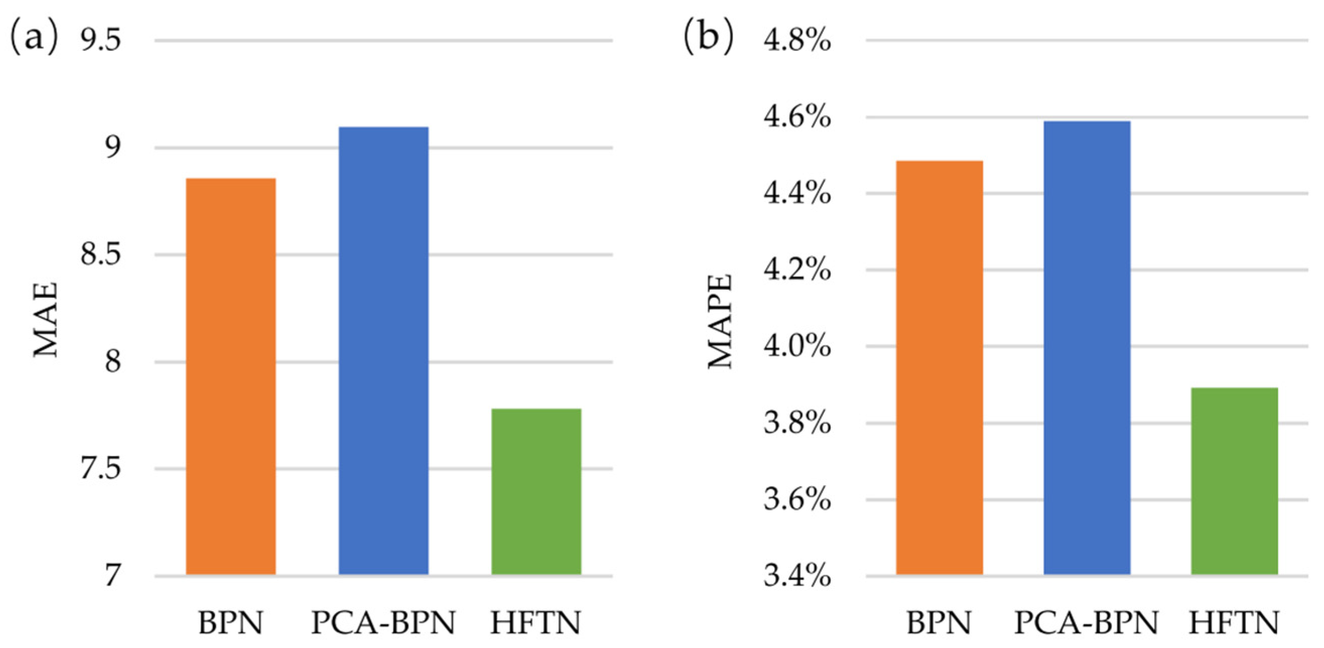
4.2. Comparison with Existing Methods

To evaluate the prediction performance of the wafer CT of the proposed methods, the advanced prediction methods of wafer CT were compared with back propagation network (BPN) and principal components analysis BPN (PCA-BPN), which proved that the HFTN could effectively extract the spatial-temporal characteristics. The experimental results are shown in Figure 4.

It can be seen from the figure that the MAE and MAPE of PCA-BPN, BPN and HFTN revealed a significant downtrend, and HFTN reconstructed the time series data in accordance with the processing areas, and integrated the spatial-temporal characteristics of the semiconductor wafer fabrication system, which had a good prediction performance for the wafer CT.

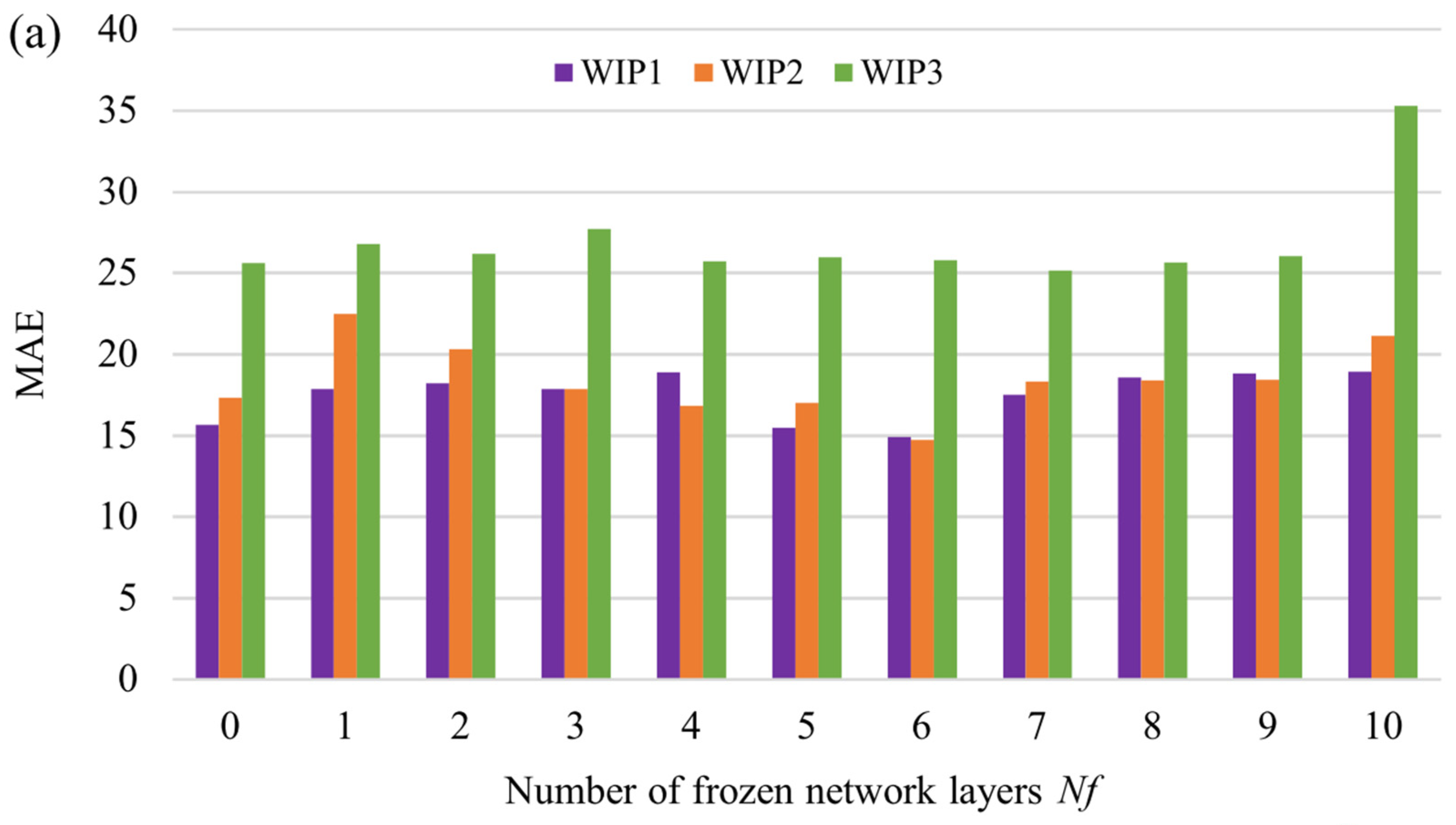
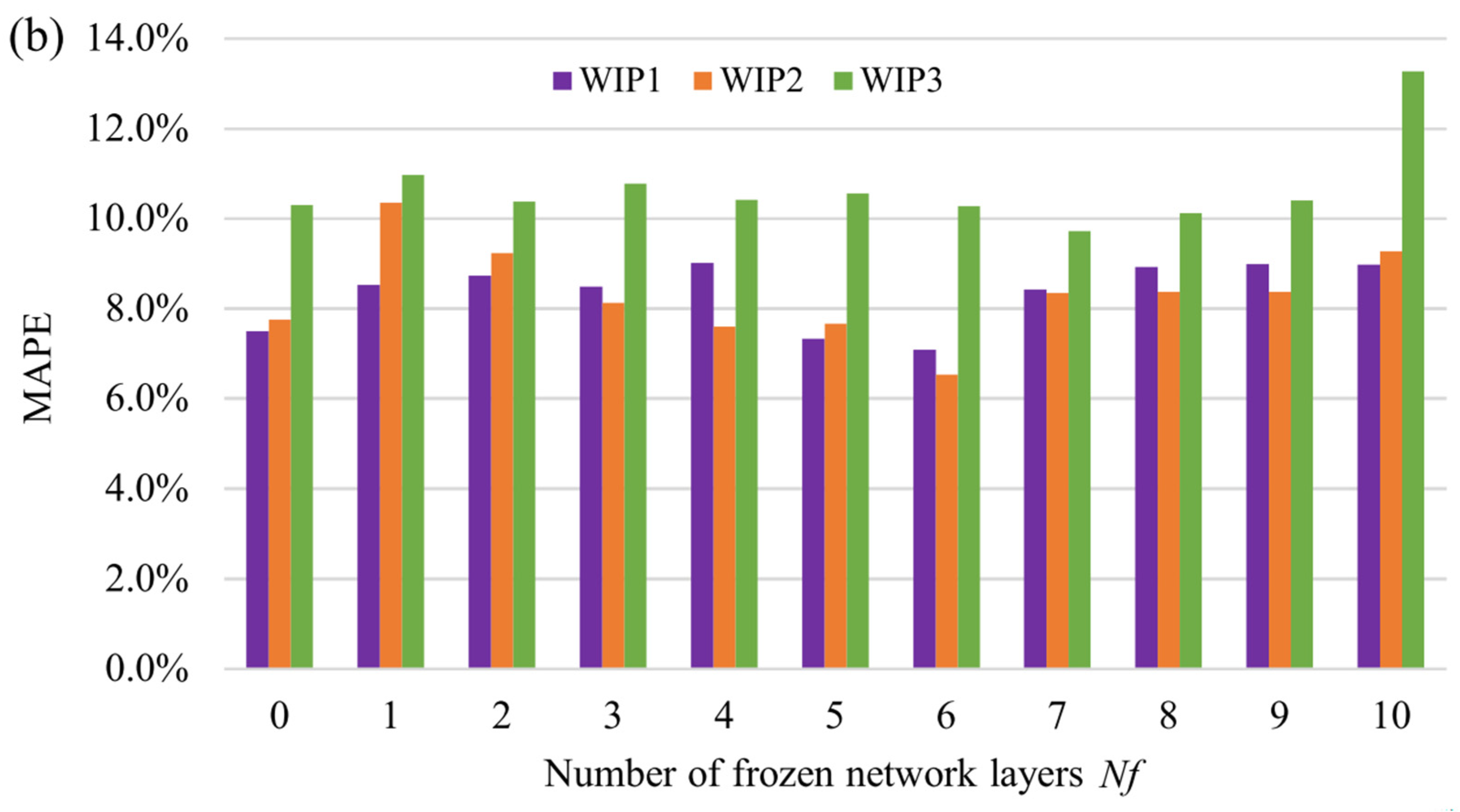
4.3. Hierarchical Optimization

In the proposed HFTN, the number of frozen network layers $N_f$ ($N_f=0,1,2,\dots ,10$) (0 represents that there is no layer frozen, 10 represents that there are 9 convolutional layers and 1 global average pooling layer involved in transfer training) had a significant impact on the transfer performance of HFTN. To look for the most appropriate parameters, a layer-by-layer experiment was conducted in this paper.

As shown in Figure 5, HFTN had a better transfer performance when $N_f=6$. As previously mentioned, the common characteristics at different WIP levels were extracted from the frozen layer. The unique characteristics at different WIP levels were extracted from the subsequent optimization layer. When the number of the frozen layers was less than six, HFTN failed to fully extract the common characteristics, and the transfer results were poor. When the number of frozen layers was greater than six, HFTN retained too many characteristic extraction ways at the original WIP levels, and failed to specifically learn the characteristics at a new WIP level. According to the structure of HFTN, the feature maps at the first six convolutional layers were larger than the feature maps at the remaining layers after average pooling twice. The common characteristics extracted from the first six layers were highly integrated into the feature maps where the unique characteristics were the underlying information. Further convolution extracted these unique characteristics that vary in different WIP levels. Therefore, the optimal number of frozen layers of the network was six, and the transfer model showed that the optimal prediction performance of CT after the sixth layer was optimized layer by layer.

5. Conclusions

In this study, the prediction of wafer CT at a new level was investigated using the transfer learning method based on the hierarchical finetuning when the WIP level changed, and its main contribution can be summarized as below:

(1)

The processing area characteristics of the multiple re-entrant flow wafer fabrication were taken into account, and the 2D convolutional neural network was utilized to extract the spatial-temporal characteristics from the wafer fabrication data, and the CT prediction of a single WIP level was achieved in this way.

(2)

The transfer learning strategy based on the hierarchical optimization and the underlying structure sharing the weights was designed to extract the common characteristics of the manufacturing system at different WIP levels. Through pooling twice, the common characteristics were highly integrated into specific characteristics. So, the finetuning training was conducted on the high-level architecture to extract the specific characteristics. Finally, the prediction of wafer CT at a new WIP level was achieved through hierarchical transfer learning.

According to the experimental results, the reorganization of input data effectively construct the spatial-temporal characteristics, and the 2D CNN architecture successfully extracts these characteristics. Moreover, the hierarchical finetuning strategy is utilized to train the layers differently in the transfer model—it helps HFTN to achieve an optimal prediction performance at different WIP levels.

Although HFTN has shown a better performance on wafer CT prediction at different WIP levels, challenges still remain that stem from the dynamic system environment. Dynamic fabrication states, except for WIP levels (such as machine failure and workers’ mistakes), also result in changes in production progress. The uncertainty makes it difficult to predict the wafer CT in the actual production environment.

As a powerful approach to reduce uncertainty, fuzzy learning has been widely applied in industry, finance, traffic, and other specific applications [34,35,36,37]. Our future work will focus on the prediction problems of wafer CT in a more actual production environment in order to explore the fluctuation rules of wafer CT with the adopted fuzzy logic-based approaches.

References

1. Uzsoy, R.; Fowler, J.W.; Moench, L. A survey of semiconductor supply chain models Part II: Demand planning, inventory management, and capacity planning. Int. J. Prod. Res. 2018, 56, 4546–4564. [Google Scholar] [CrossRef]
2. Chidambaram, P.R.; Bowen, C.; Chakravarthi, S.; Machala, C.; Wise, R. Fundamentals of silicon material properties for successful exploitation of strain engineering in modern CMOS manufacturing. IEEE Trans. Electron. Devices 2006, 53, 944–964. [Google Scholar] [CrossRef]
3. Moench, L.; Uzsoy, R.; Fowler, J.W. A survey of semiconductor supply chain models part III: Master planning, production planning, and demand fulfilment. Int. J. Prod. Res. 2018, 56, 4565–4584. [Google Scholar] [CrossRef]
4. Wang, J.; Xu, C.; Zhang, J.; Zhong, R. Big data analytics for intelligent manufacturing systems: A review. J. Manuf. Syst. 2021, in press. [Google Scholar] [CrossRef]
5. Hopp, W.J.; Spearman, M.L. Factory Physics: Foundations of Manufacturing Management, 2nd ed.; Irwin/McGraw-Hill: Boston, MA, USA, 2001. [Google Scholar]
6. Wang, J.; Zheng, P.; Zhang, J. Big data analytics for cycle time related feature selection in the semiconductor wafer fabrication system. Comput. Ind. Eng. 2020, 143, 106362. [Google Scholar] [CrossRef]
7. Wang, J.; Yang, J.; Zhang, J.; Wang, X.; Zhang, W. Big data driven cycle time parallel prediction for production planning in wafer manufacturing. Enterp. Inf. Syst. 2018, 12, 714–732. [Google Scholar] [CrossRef]
8. Zhang, C.; Bard, J.F.; Chacon, R. Controlling work in process during semiconductor assembly and test operations. Int. J. Prod. Res. 2017, 55, 7251–7275. [Google Scholar] [CrossRef] [Green Version]
9. Wang, J.; Xu, C.; Yang, Z.; Zhang, J.; Li, X. Deformable convolutional networks for efficient mixed-type wafer defect pattern recognition. IEEE Trans. Semicond. Manuf. 2020, 33, 587–596. [Google Scholar] [CrossRef]
10. Yang, F.; Ankenman, B.E.; Nelson, B.L. Estimating cycle time percentile curves for manufacturing systems via simulation. Inf. J. Comput. 2008, 20, 628–643. [Google Scholar] [CrossRef]
11. Tai, Y.T.; Pearn, W.L.; Lee, J.H. Cycle time estimation for semiconductor final testing processes with Weibull-distributed waiting time. Int. J. Prod. Res. 2012, 50, 581–592. [Google Scholar] [CrossRef]
12. Sha, D.Y.; Storch, R.L.; Liu, C.H. Development of a regression-based method with case-based tuning to solve the due date assignment problem. Int. J. Prod. Res. 2007, 45, 65–82. [Google Scholar] [CrossRef]
13. Schelasin, R. Using static capacity modeling and queuing theory equations to predict factory cycle time performance in semiconductor manufacturing. In Proceedings of the 2011 Winter Simulation Conference, Phoenix, AZ, USA, 11–14 December 2011; pp. 2040–2049. [Google Scholar] [CrossRef]
14. Guo, Z.; Baruah, S.K. A neurodynamic approach for real-time scheduling via maximizing piecewise linear utility. IEEE Trans. Neural Netw. Learn. Syst. 2016, 27, 238–248. [Google Scholar] [CrossRef] [PubMed]
15. Li, X.; Bai, R. Freight vehicle travel time prediction using gradient boosting regression tree. In Proceedings of the 2016 15th IEEE International Conference on Machine Learning and Applications (ICMLA), New York, NY, USA, 18–20 December 2016; pp. 1010–1015. [Google Scholar] [CrossRef]
16. Ke, G.; Meng, Q.; Finley, T.; Wang, T.; Chen, W.; Ma, W.; Ye, Q.; Liu, T.Y. Lightgbm: A highly efficient gradient boosting decision tree. Adv. Neural Inf. Process. Syst. 2017, 30, 3146–3154. [Google Scholar]
17. Liu, J.; Zio, E. SVM hyperparameters tuning for recursive multi-step-ahead prediction. Neural Comput. Appl. 2017, 28, 3749–3763. [Google Scholar] [CrossRef]
18. Chu, Z.; Zhu, D.; Yang, S.X. Observer-based adaptive neural network trajectory tracking control for remotely operated vehicle. IEEE Trans. Neural Netw. Learn. Syst. 2017, 28, 1633–1645. [Google Scholar] [CrossRef]
19. Backus, P.; Janakiram, M.; Mowzoon, S.; Runger, G.C.; Bhargava, A. Factory cycle-time prediction with a data-mining approach. IEEE Trans. Semicond. Manuf. 2006, 19, 252–258. [Google Scholar] [CrossRef]
20. Pearn, W.L.; Chung, S.H.; Lai, C.A. Due-date assignment for wafer fabrication under demand variate environment. IEEE Trans. Semicond. Manuf. 2007, 20, 165–175. [Google Scholar] [CrossRef]
21. Tirkel, I. Forecasting flow time in semiconductor manufacturing using knowledge discovery in databases. Int. J. Prod. Res. 2013, 51, 5536–5548. [Google Scholar] [CrossRef]
22. Chang, P.C.; Liao, T.W. Combining SOM and fuzzy rule base for flow time prediction in semiconductor manufacturing factory. Appl. Soft. Comput. 2006, 6, 198–206. [Google Scholar] [CrossRef]
23. Chen, T.; Wang, Y.C. Incorporating the FCM–BPN approach with nonlinear programming for internal due date assignment in a wafer fabrication plant. Robot. Com.-Int. Manuf. 2010, 26, 83–91. [Google Scholar] [CrossRef]
24. Zhu, X.; Qiao, F. Cycle time prediction method of wafer fabrication system based on industrial big data. Comput. Integ. Manuf. Sys. 2017, 23, 2172–2179. [Google Scholar] [CrossRef]
25. Wang, J.; Zhang, J.; Wang, X. Bilateral LSTM: A two-dimensional long short-term memory model with multiply memory units for short-term cycle time forecasting in re-entrant manufacturing systems. IEEE Trans. Ind. Inf. 2018, 14, 748–758. [Google Scholar] [CrossRef]
26. Bai, Y.; Li, C.; Sun, Z.; Chen, H. Deep neural network for manufacturing quality prediction. In Proceedings of the 2017 Prognostics and System Health Management Conference (phm-Harbin), Harbin, China, 9–12 July 2017; pp. 307–311. [Google Scholar]
27. Wang, C.; Jiang, P. Deep neural networks based order completion time prediction by using real-time job shop RFID data. J. Intell. Manuf. 2019, 30, 1303–1318. [Google Scholar] [CrossRef]
28. Sun, C.; Ma, M.; Zhao, Z.; Tian, S.; Yan, R.; Chen, X. Deep transfer learning based on sparse autoencoder for remaining useful life prediction of tool in manufacturing. IEEE Trans. Ind. Inform. 2019, 15, 2416–2425. [Google Scholar] [CrossRef]
29. Xu, C.; Wang, J.; Zhang, J.; Li, X. Anomaly detection of power consumption in yarn spinning using transfer learning. Comput. Ind. Eng. 2021, 152, 107015. [Google Scholar] [CrossRef]
30. Wang, R.; Peng, C.; Gao, J.; Gao, Z.; Jiang, H. A dilated convolution network-based LSTM model for multi-step prediction of chaotic time series. Comput. Appl. Math. 2020, 39, 30. [Google Scholar] [CrossRef]
31. Xiao, Y.; Yin, H.; Zhang, Y.; Qi, H.; Zhang, Y.; Liu, Z. A dual-stage attention-based Conv-LSTM network for spatio-temporal correlation and multivariate time series prediction. Int. J. Intell. Syst. 2021, 36, 2036–2057. [Google Scholar] [CrossRef]
32. Wang, J.; Xu, C.; Dai, L.; Zhang, J.; Zhong, R. An unequal learning approach for 3D point cloud segmentation. IEEE Trans. Ind. Inf. 2021, 1. [Google Scholar] [CrossRef]
33. Goodfellow, I.; Bengio, Y.; Courville, A. Deep Learning; Adaptive Computation and Machine Learning; The MIT Press: Cambridge, MA, USA, 2016. [Google Scholar]
34. Chen, H.; Yang, B.; Wang, G.; Liu, J.; Xu, X.; Wang, S.; Liu, D. A novel bankruptcy prediction model based on an adaptive fuzzy K-Nearest neighbor method. Knowl.-Based Syst. 2011, 24, 1348–1359. [Google Scholar] [CrossRef]
35. Versaci, M.; Morabito, F.C. Fuzzy time series approach for disruption prediction in tokamak reactors. IEEE Trans. Magn. 2003, 39, 1503–1506. [Google Scholar] [CrossRef]
36. Wang, H.; Zheng, L.; Meng, X. Traffic accidents prediction model based on fuzzy logic. Commun. Comput. Inf. Sci. 2011, 201, 101–108. [Google Scholar] [CrossRef]
37. Zhu, B.; Chen, M.; Wade, N.; Ran, L. A prediction model for wind farm power generation based on fuzzy modeling. Procedia Environ. Sci. 2012, 12, 122–129. [Google Scholar] [CrossRef] [Green Version]
Figure 1. Huge and complex semiconductor wafer fabrication system and cycle time in different quarters.
Mathematics 09 02039 g001
Figure 2. Architecture of the proposed hierarchical finetuning transfer network.
Mathematics 09 02039 g002
Figure 3. Reorganize the time series data to a feature map through the block splicing of different processing areas.
Mathematics 09 02039 g003
Figure 4. The CT prediction with three methods (BPN, PCA-BPN, and HFTN): (a) MAE analysis; (b) MAPE analysis.
Mathematics 09 02039 g004
Figure 5. Hierarchical optimization of the number of frozen network layers, N f , at three WIP levels: (a) MAE analysis and (b) MAPE analysis.
Mathematics 09 02039 g005aMathematics 09 02039 g005b