1. Introduction
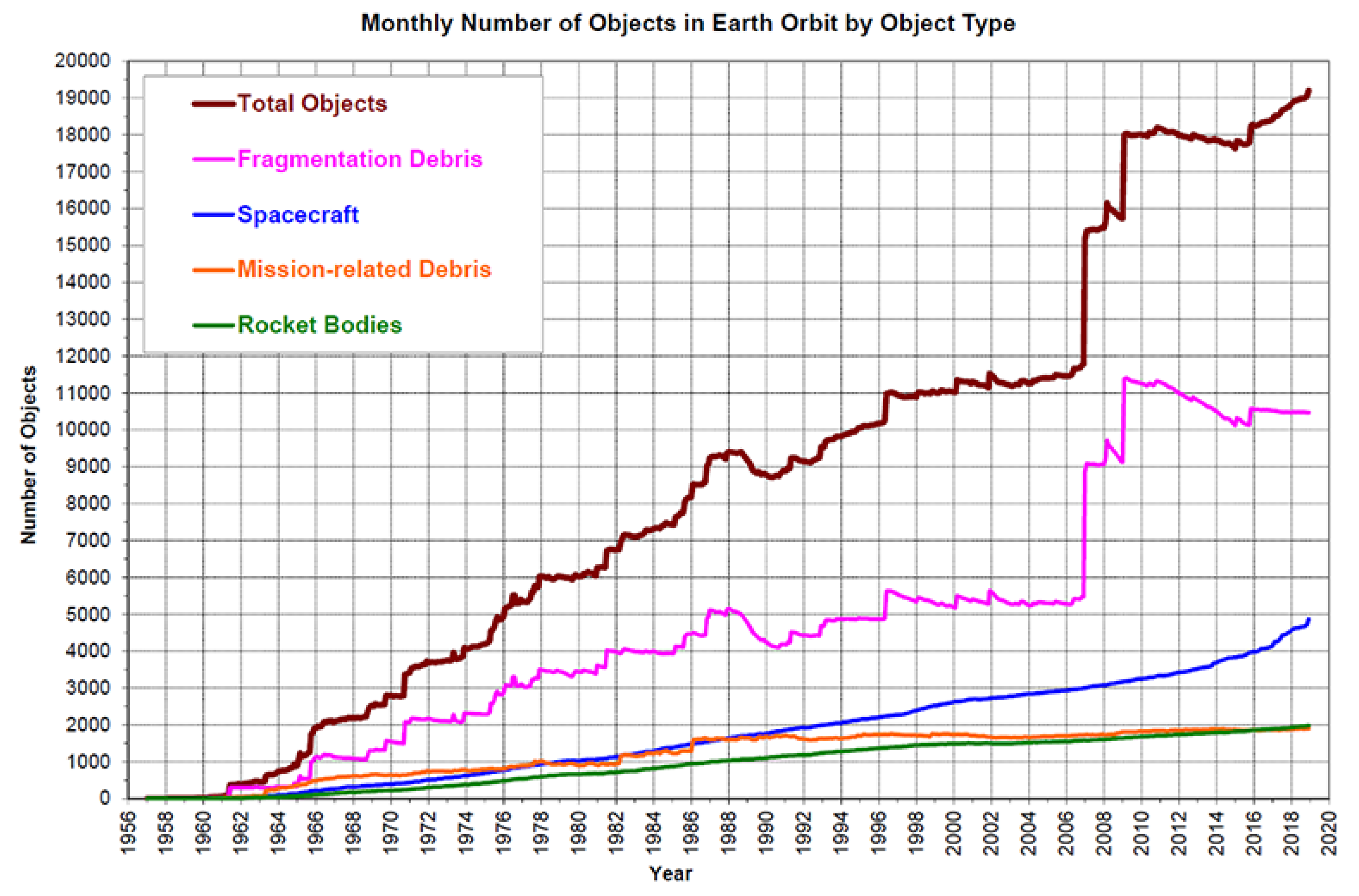
The number of satellites and artificial objects orbiting in space around the earth has grown exponentially in recent decades due to the reduction of production costs and technological advances that facilitate their launch. Thus, the number of artificial objects orbiting the Earth in the year 2000 has increased from 11,000 to 19,500 objects in the year 2019, with a much higher forecast for the coming years [
1], as seen in
Table 1 published by the European Space Agency (ESA) about the debris figures [
2]. Consequently, the disproportionate increase in space debris over the years, as seen in
Figure 1, generates a greater risk of collision between satellites, which in turn generates more debris and more risk of collision. This growth highlights the need for positional control of the satellite in space so that it does not collide with any other object and cause major damage.
The debris problem has been a matter of study and concern since the United Nations published a report in 1999 warning about this forthcoming problem [
3], focusing its information on orbital debris measurements, modeling, risk assessments, and mitigation measures.
The United States as the lead country, and NASA, has a specific government organization designated to control space debris, The United States Government Orbital Debris Mitigation Standard Practices (ODMSP) [
4]. Among its tasks is the mission of issuing reports and generating control mechanisms to minimize the discharge of space debris in case of collision as well as a guide of good practices for space operations to promote efficient and effective space safety practices.
The loss of control of satellites in their orbits can generate collisions like the 2009 accident where the American satellite US Iridium-33 communication satellite and the inactive Russian Kosmos-2251 collided with each other [
5], or more recently, in 2021, where the Chinese rocket Long March 5B entered the Earth’s atmosphere uncontrolled and at risk of causing numerous damages [
6].
The prediction of orbits in space objects and the calculation of their error has been a topic addressed by several studies applying numerous artificial intelligence techniques. The ease of finding reliable data on object positions in space provided by numerous space agencies [
8,
9,
10], makes more reliable the use of machine learning techniques combined with Big Data that increase the reliability of the results obtained. In this scope, machine learning algorithms provide data modelling based on large historical data, providing in some cases a different prediction from physical evidence [
11].
In this regard, it is worth mentioning the study presented in [
12] on the orbit prediction of 11 satellites using machine learning techniques, specifically a support vector machine (SVM) model applied to data obtained from TLE catalog. In this case, the measurements were uniform, so results demonstrated an improvement in the orbit prediction accuracy. SVM has been widely used to predict orbit errors as in [
13,
14], improving the orbit prediction accuracy learning from historical prediction errors.
Other machine learning techniques have been used to improve orbit prediction accuracy as in [
15] implementing LSTM networks to provide atmospheric density predictions, in [
16] convolutional neural networks to work with special images to detect space objects, or in [
17,
18,
19] where neural networks were used, for example, to explore the solar gravity-driven orbital transfers in the Martian system.
These studies started with a uniform, process-ready dataset. This is usually not the real case, where measurements and data require deep filtering, or even, as in our study, an intermediate data prediction process to complete the dataset added to these machine learning techniques, we have used prediction techniques based on median values from the dataset to fill in those gaps of missing measurements. This way we will be able to provide more accuracy when calculating our orbit’s parameters, and so the highest accuracy on our error calculation and prediction model.
2. Data Collection and Preprocessing Stage
For this experiment, we have used the satellite data available for download at Kaggle website [
20]. For each satellite, we know its ID and the sequence of positions (x,y,z) through which it passed over time with the timestamp of the moment it did so. We also have the velocity of each of the dimensions that will be used in future works.
The dataset has the positions of 600 satellites between 1 and 24 January, 2014. It has in total about 503,227 rows and one would expect to have about 839 positions for each satellite. However, this is not the case and each satellite has a different number of positions (some more some less) and even the positions of the satellites are recorded at different times during the passage of time. This makes it difficult, for example, to calculate the error in the orbit of a satellite or even to detect collisions between satellites as we will tackle in the next sections.
For this reason, in this article we decided to create a prediction algorithm to estimate those measurements missing and help to better accuracy in the ellipse calculations along with the estimated error provided among all ellipses.
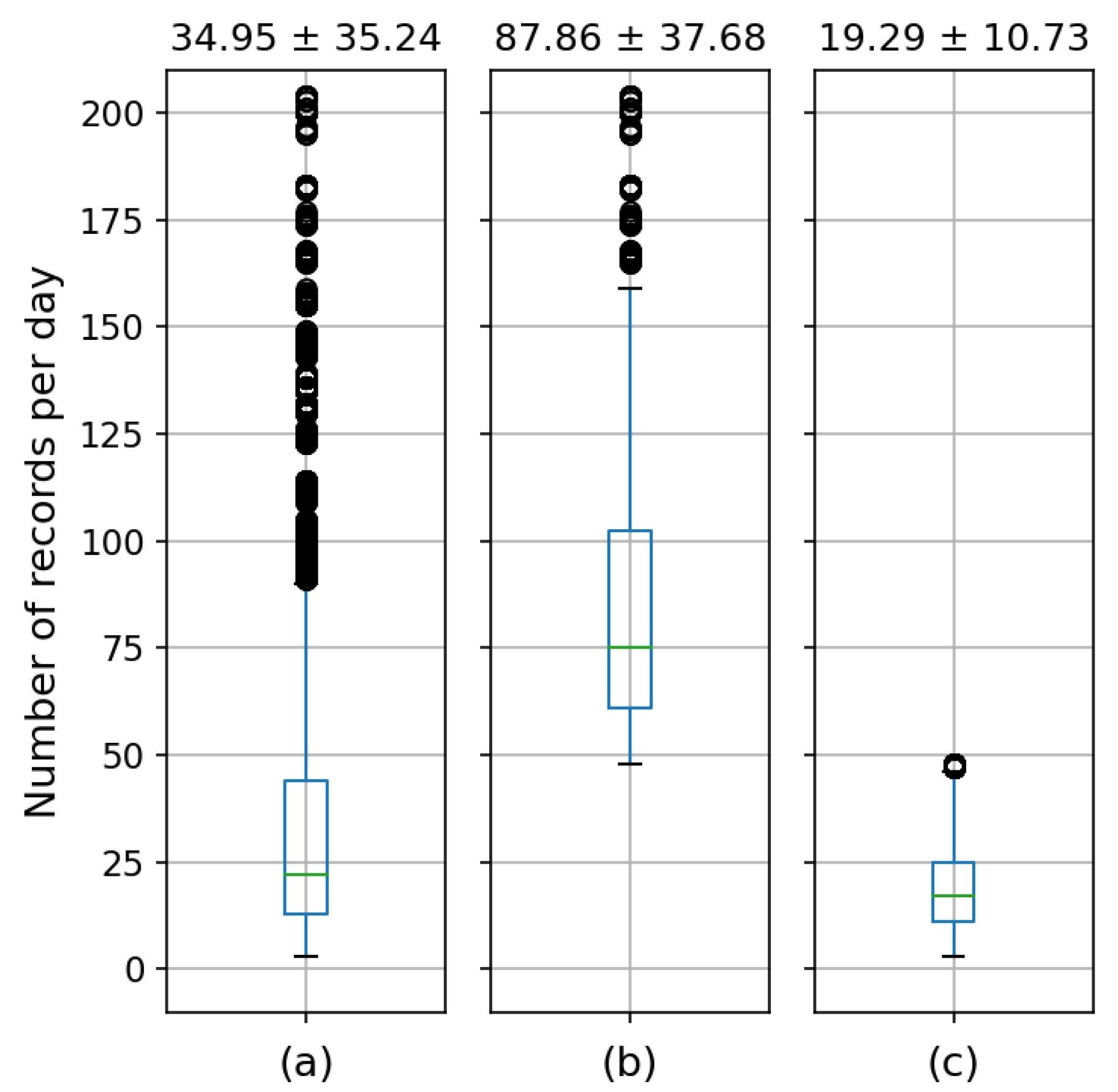
In this article, we will work with the positions (x,y,z) of 137 satellites with all their positions recorded in no more than 30 min. This is achieved by calculating the differences between consecutive timestamps. This is how we managed to have from each satellite about 50 samples per day (2 every one hour).
Figure 2 shows the mean ± deviation and the box plot corresponding to the number of records that the satellites have per day for (a) the total sample, (b) the 137 selected satellites and (c) for the rest. As seen in (b), by having at least one record every half hour, we ensure that we have the most complete track of the satellites to be analyzed.
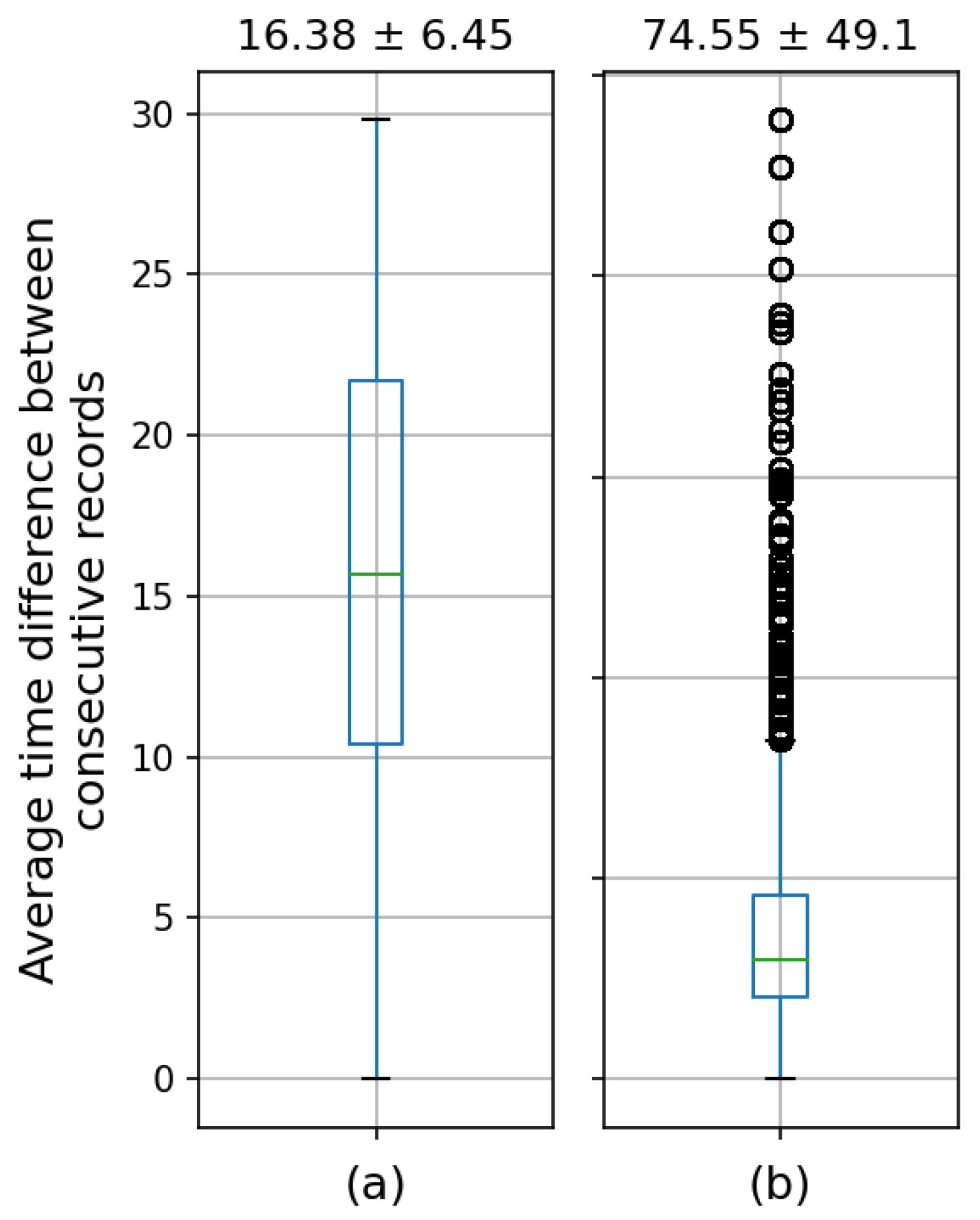
As seen in
Figure 3, for those 137 satellites that have been selected, the differences in time between records are somewhat more stable. They do not exceed 30 min and are around 16.38 ± 6.45 min. On the other hand, for the remaining 463 satellites of the total set, the differences vary greatly with outliers. In the experimental section, we will reflect the differences between these 137 satellites with stable measures, with the others to minimize the prediction error in our position’s estimation.
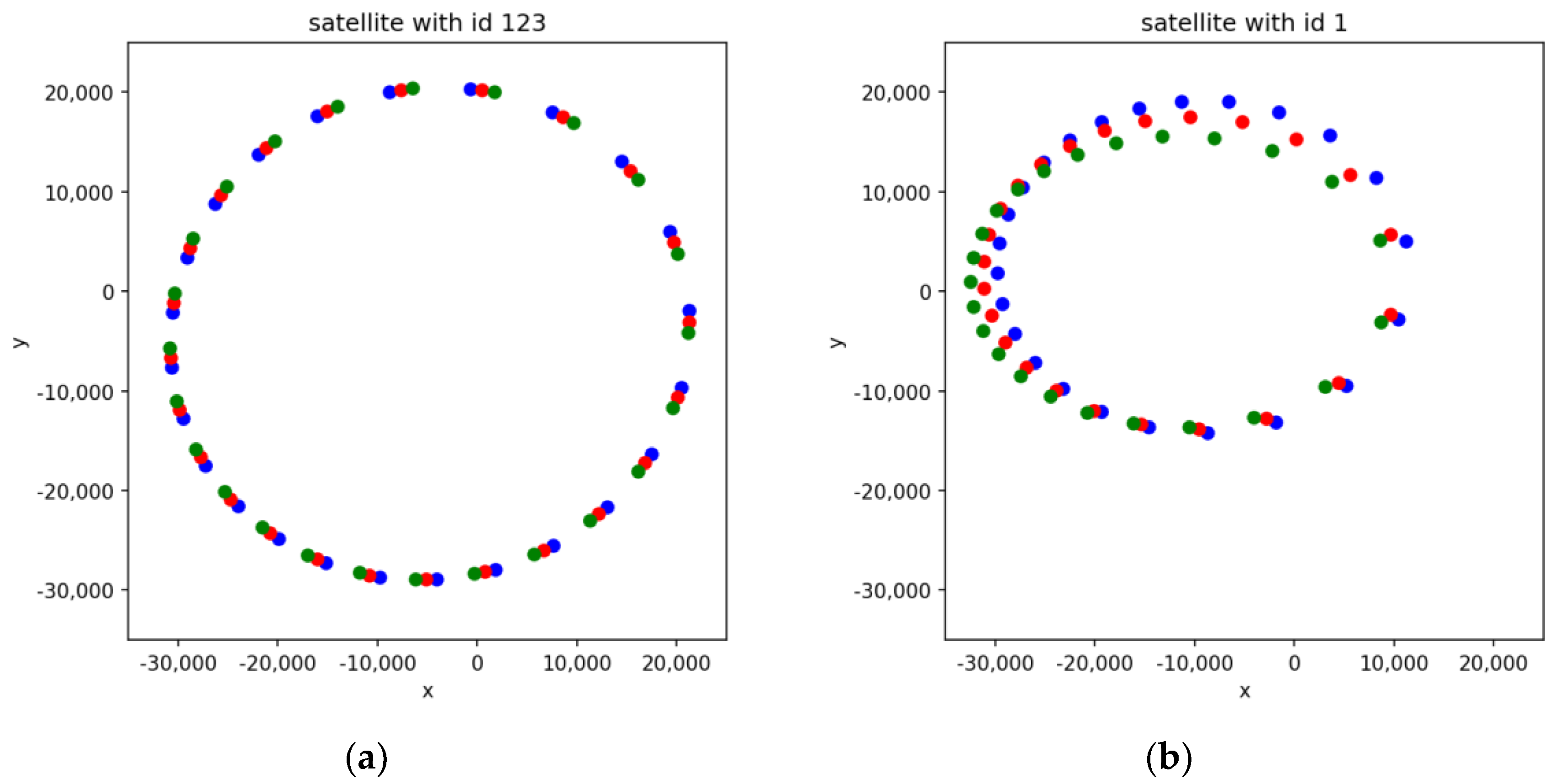
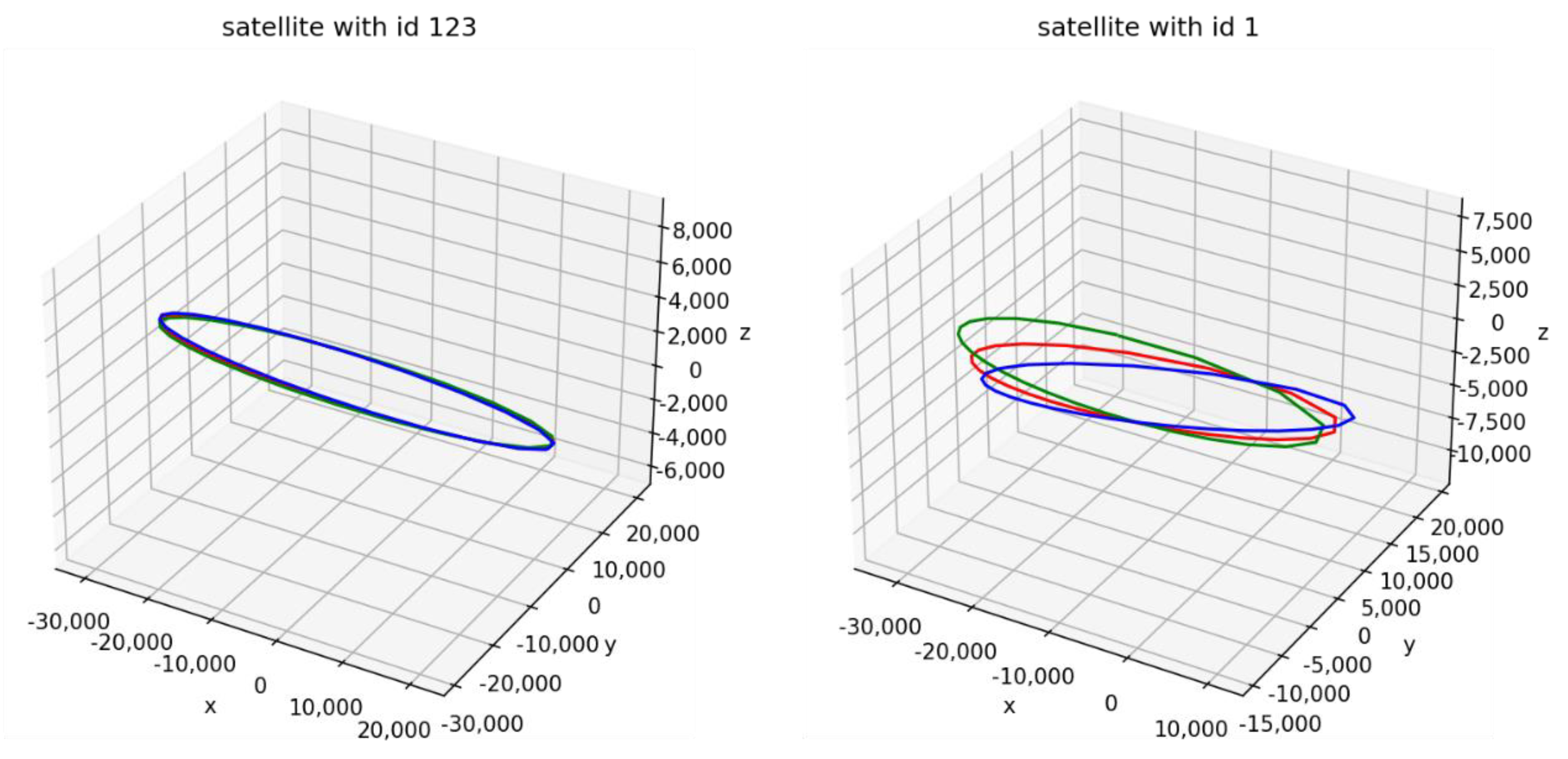
Figure 4a shows the differences in (x,y) of the satellite with id 123 at the beginning (blue), at an intermediate point (red) and at the end of the timeline (green). The differences in this particular case are due to the times at which the positions are recorded. However, these differences may also be due to errors during the satellite orbit as seen in
Figure 4b.
These differences may even be due to accelerations that the satellite undergoes during the passage of time.
Figure 5 shows the differences of the same two satellites of
Figure 4, taking into account in this case the positions in three dimensions.
To calculate the error of the satellite orbits, it is essential to approximate the ellipse of the satellite motion with the available data (see
Section 3.2) and to compare all the satellite cycles with the ellipse approximation.
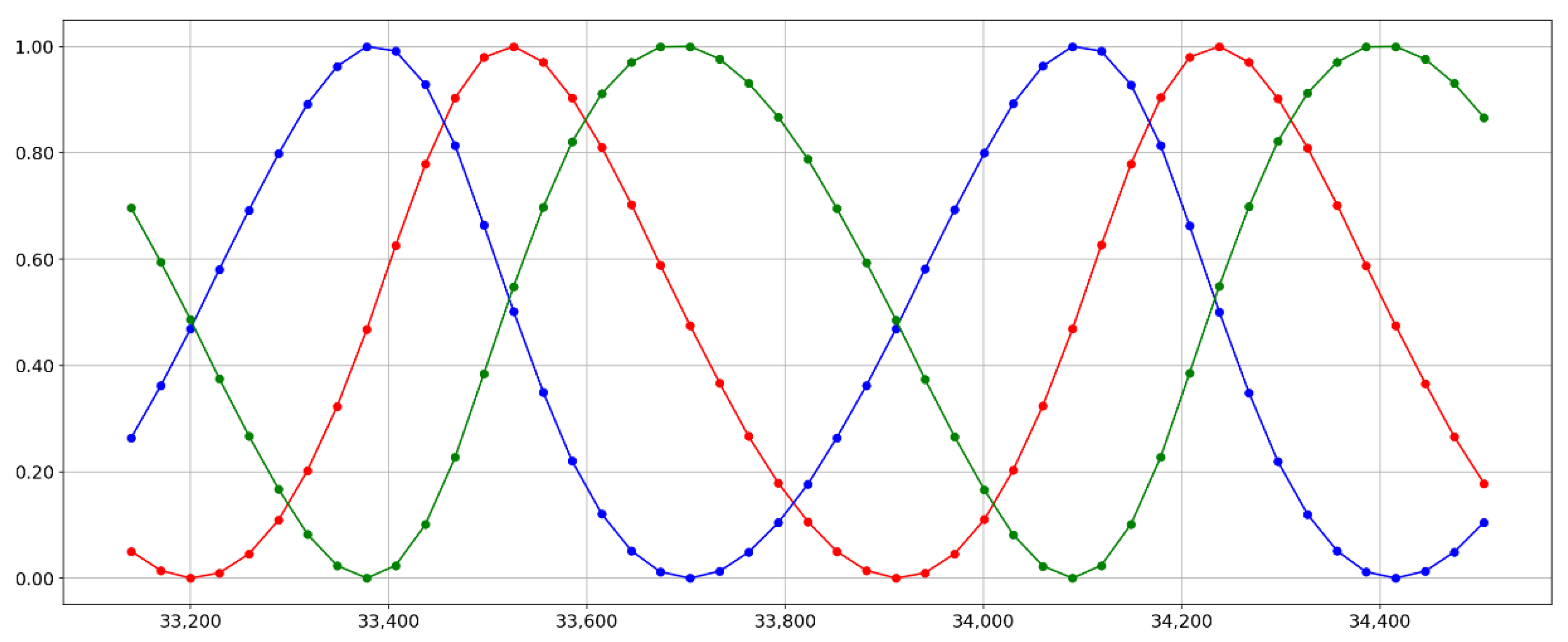
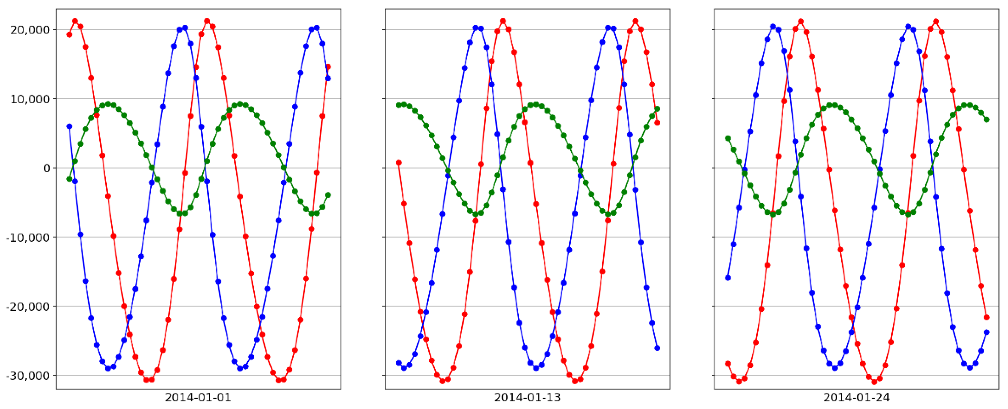
Figure 6 shows in signal form the motion of a satellite in its three dimensions at three different times. As seen in the figure, the positions of the same satellite on three different days are not comparable. Therefore, the key is to determine the “cycle” of the satellite to slice the signal and this can be solved by obtaining the inflection points. The difficulty lies in the triple dimension of the data, as obtaining the 3D inflection points is not an easy thing to do [
21].
Figure 6 shows the signal (x,y,z) of a satellite scaled between (0,1)for easy visualization and the position of the satellite in each dimension per time instant. As seen, it is not the same instant in all three dimensions when the satellite is returning to its position. Both aspects (those mentioned in
Figure 6 and
Figure 7) make data processing and satellite position prediction difficult.
However, in the case of satellites, it is sufficient to obtain the peaks of the signal in one of the three dimensions (e.g., x), obtaining the local maxima by a simple comparison of neighboring values. In this way, the satellite cycles can be obtained and the beginning and end of the signal can be discarded to obtain complete cycles of the satellite path.
3. Fitting the Points and Finding the Errors
Once the data have been filtered and preprocessed as we mentioned in the previous section, we used the minimum squared method to fit the points to an ellipse and find the center and the axis of said ellipse.
To do so, we applied python and Matlab languages as we will see in the next sections.
3.1. Least Squared Method
Least squares is a numerical analysis technique framed within mathematical optimization, in which, given a set of ordered pairs—independent variable, dependent variable—and a family of functions, an attempt is made to find the continuous function, within that family, that best approximates the data (a “best fit”), according to the criterion of least squared error.
In its simplest form, it attempts to minimize the sum of squares of the differences in the ordinates (called residuals) between the points generated by the chosen function and the corresponding values in the data. Specifically, it is called least mean squares (LMS) when the number of measured data is 1 and the gradient descent method is used to minimize the squared residual. It can be shown that LMS minimizes the expected squared residual, with the minimum number of operations (per iteration), but requires a large number of iterations to converge.
From a statistical point of view, an implicit requirement for the least squares method to work is that the errors of each measurement are randomly distributed. The Gauss–Markov theorem proves that least squares estimators are unbiased and that the data sampling does not have to conform, for example, to a normal distribution.
The way used to minimize the geometric distance of the points to the ellipse, for which it will be necessary to use the parametric representation of the ellipse [
22].
Let
a set of points in
,
a representation of the ellipse, and
the geometric distance of the points to the ellipse, then we want to find the ellipse such that
Another possibility is to represent the ellipse by means of its parametric equations:
Which in vector form, we can write as:
where
. As the axes can be any axes, we will use the representation:
where
is the rotation matrix and
is a diagonal matrix. Both are written below:
Then, in terms of the chosen representation, the ellipse is characterized as follows:
Thus, the distance from a point to the conic can be defined as:
In our case, the limitation presented with this method is basically that it has an error in itself due to the way it is calculated. There are different methods that could be contrasted when there is enough data from the same satellite and above all that we only have information of what is supposed to be the CM of the satellite, and not its physical extensions. The mathematical programming of the least squares is based on the code written in Matlab by Richard Brown [
23], who freely allows its use with slight variations in order to get the expected results
3.2. Least Squared Method Application
According to all this, we have applied the fitEllipse(x,y) function of python which receives a set of points with its x and y coordinates and returns the parameters of the ellipse that best fits into these points and the coordinates of the center of the ellipse and compared its results with the Matlab results.
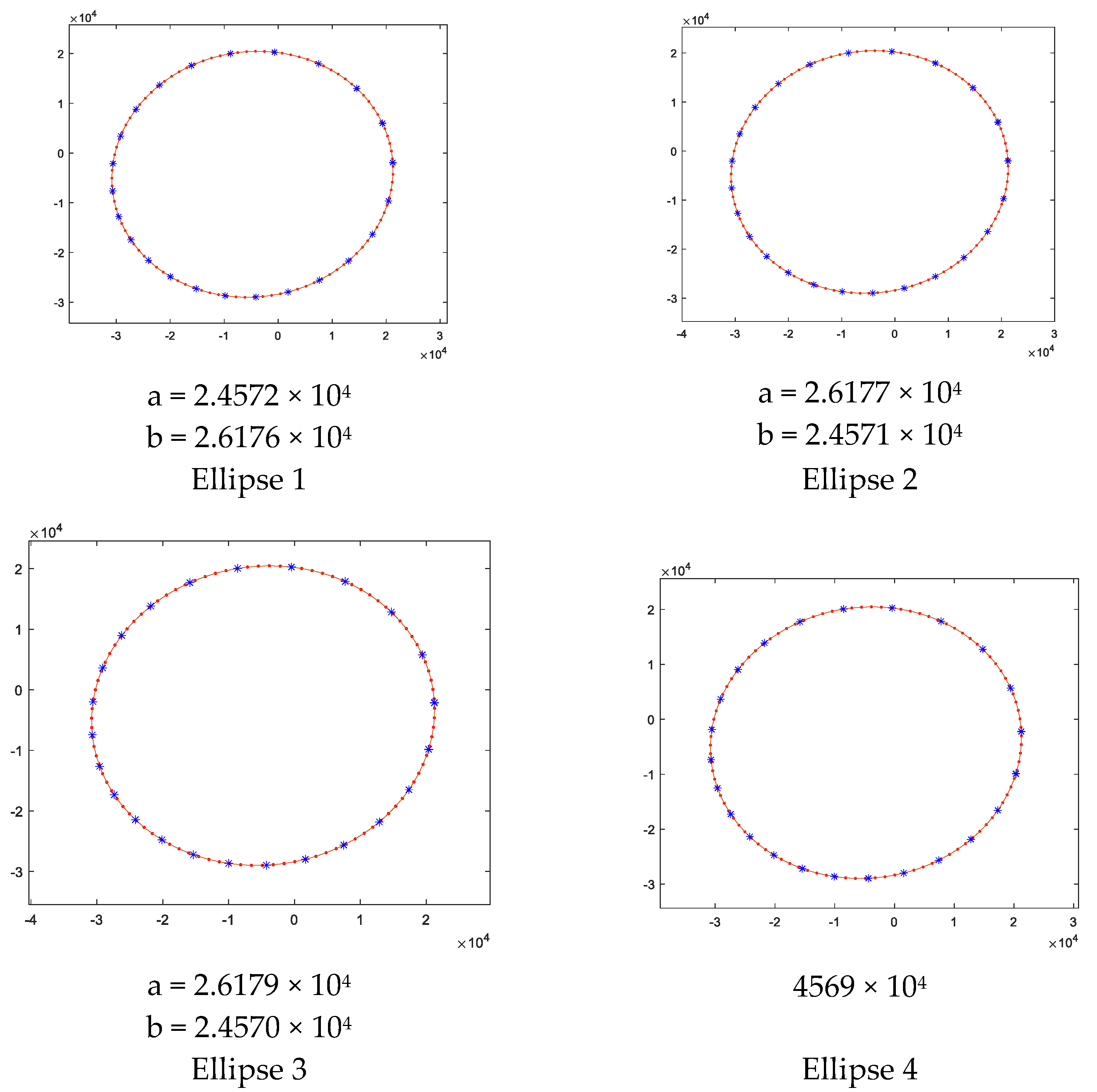
For every trajectory, we computed the center position of the 3D elliptical trajectory and the size of the two axis, a and b, as the more robust measurement of the quality of the least square approximation. These data will be not too sensitive to small changes in any spurious data.
The same satellite evaluated its trajectory in different moments dealt with these results presented in
Figure 8.
Because of the changes in the trajectory, we evaluated for the same satellite, its trajectory in different moments and evaluated those parameters. Based on the database information and the exploratory analysis performed, one satellite lasts 12 h in performing a full orbit, so we have in 26 days, 48 full orbits to compute the error among them.
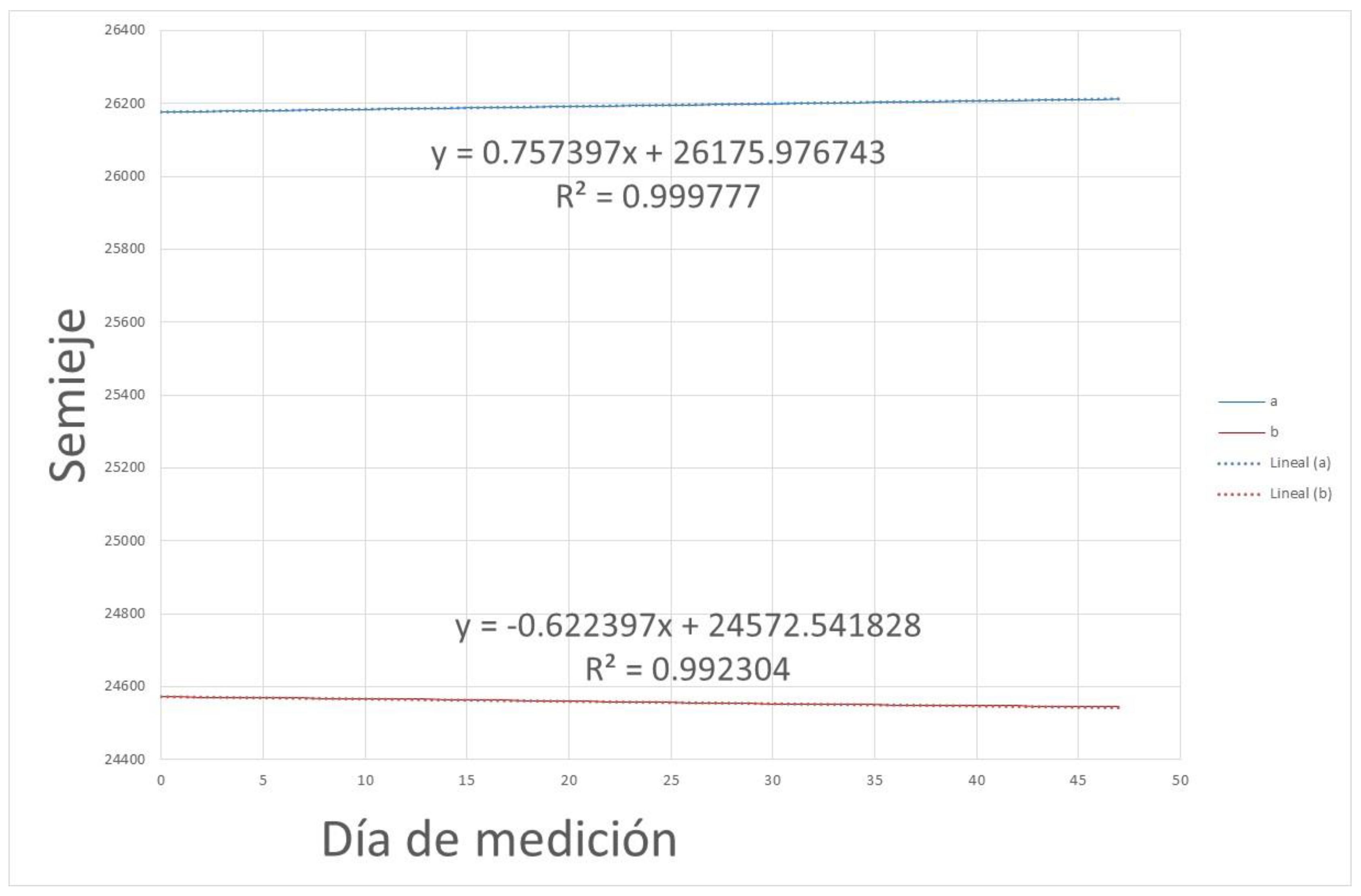
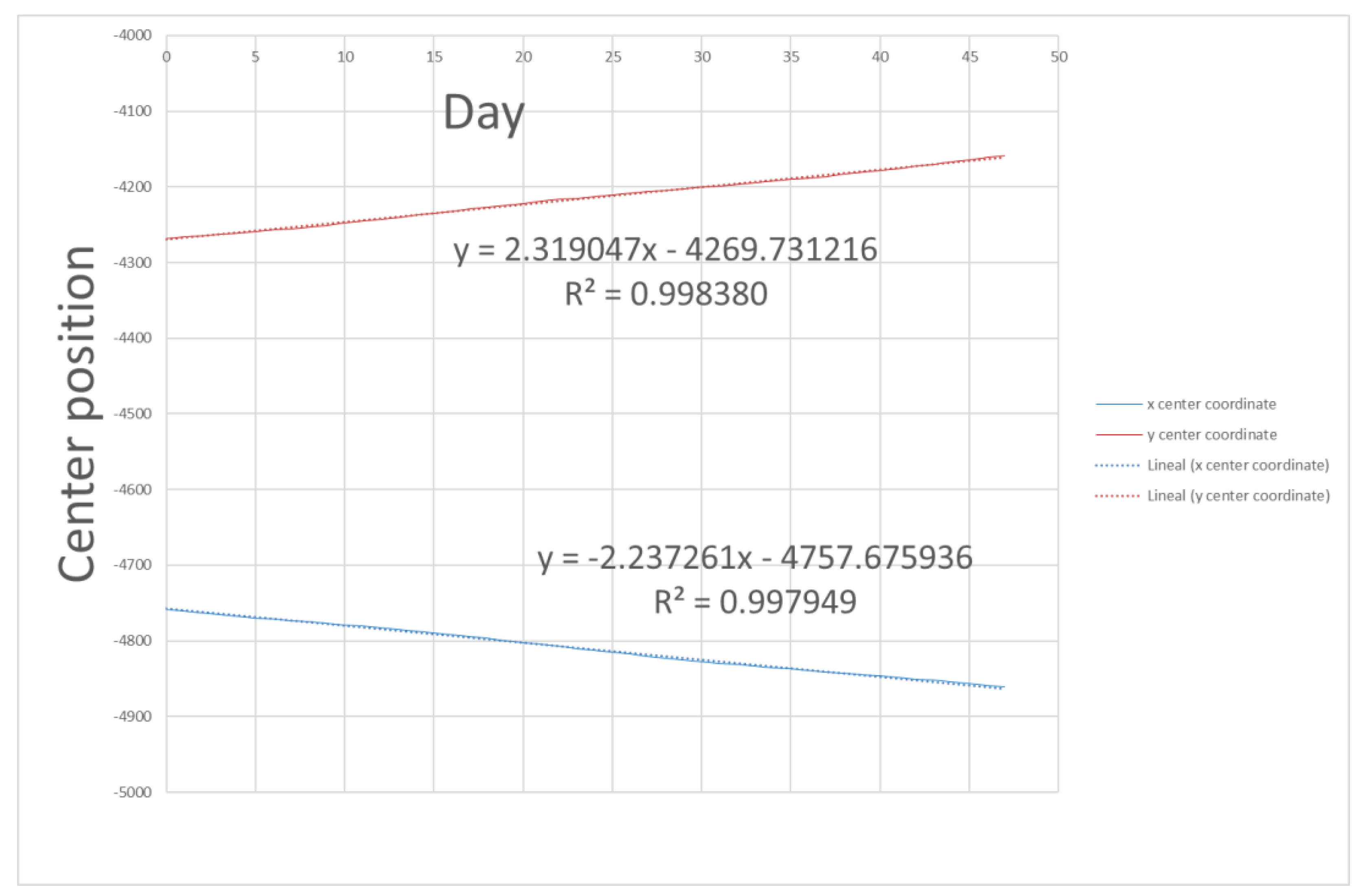
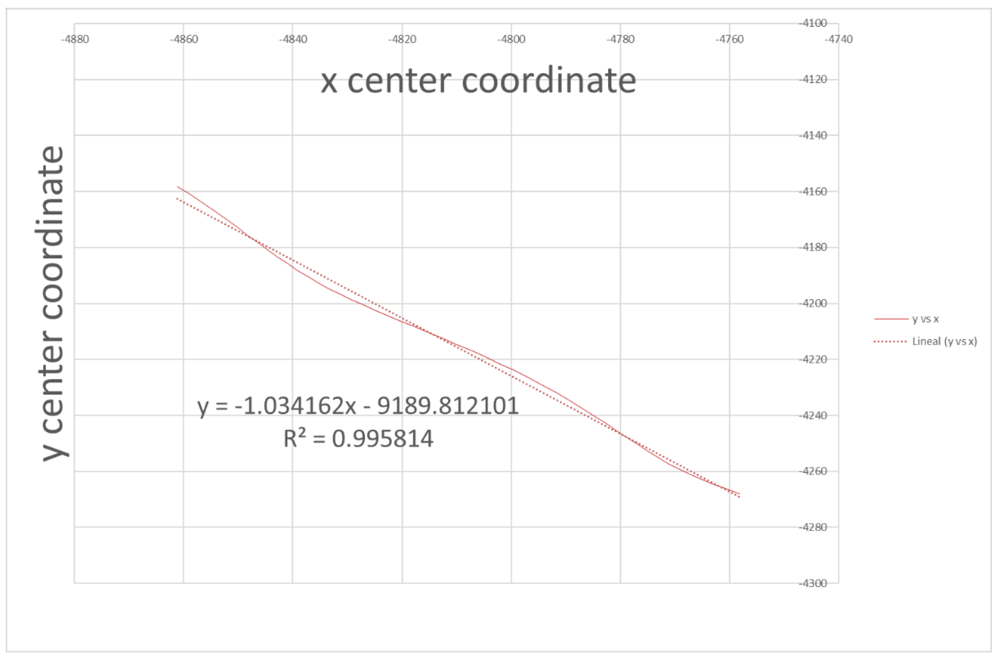
Then, we plotted the center position coordinates (x,y) of the ellipse trajectory versus the day of measurement. Approximating the points to a straight line results in two graphs with practically opposite slopes, which shows an opposite but homogeneous trend in the two coordinates. When one varies, the other varies with the same relationship in the opposite direction. This is shown in
Figure 9.
As seen in
Figure 9, a linear dependence is observed in the slope of the two coordinates of the center of the ellipse, the trajectory of the satellite. This dependence is possibly caused by the satellite’s own control. Although these data are known to the owners of the satellite, they are not public. A satellite tracking and position prediction will help to avoid collisions. Therefore, the goodness of the determination of such an approach is determined. To begin with, we represent the dependence of these coordinates on each other as seen in
Figure 10.
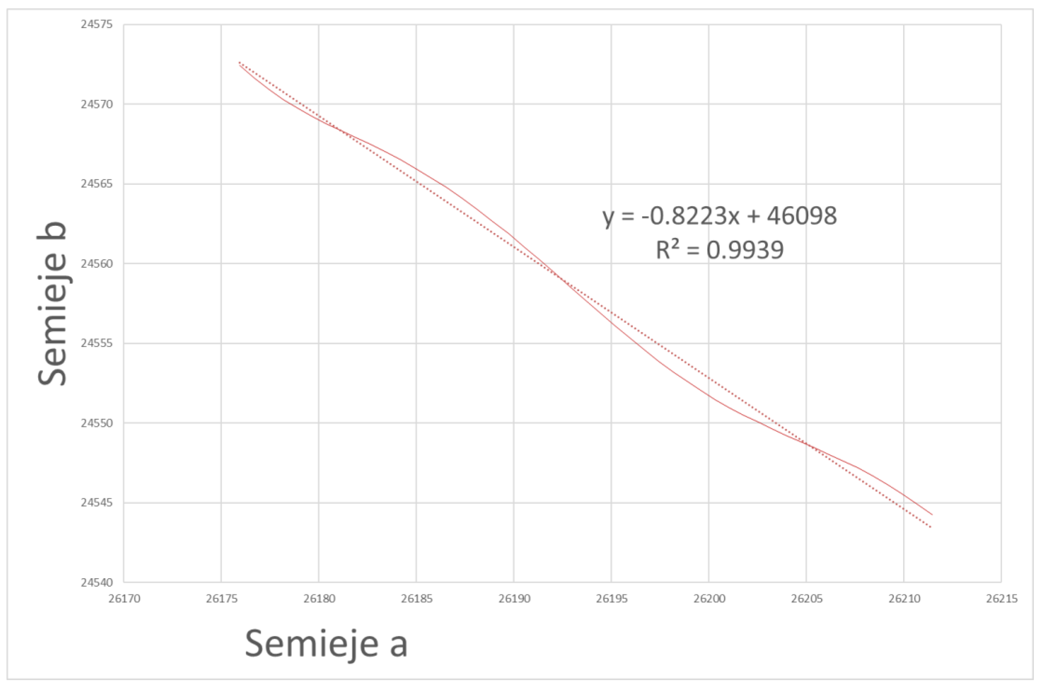
Since the latter equation has a slope of 1, it indicates that the two coordinates x and y vary approximately equally. What one increases is what increases the other. However, when the semi-axes of the ellipse are represented, it turns out as seen in
Figure 11.
There is also a dependence between the two semi-axes of the satellite trajectory. Therefore, we are determining one of the parameters that can best help us to predict the position of the satellite based on the public data. Representing the two semi-axes graphically, it follows as seen in
Figure 12.
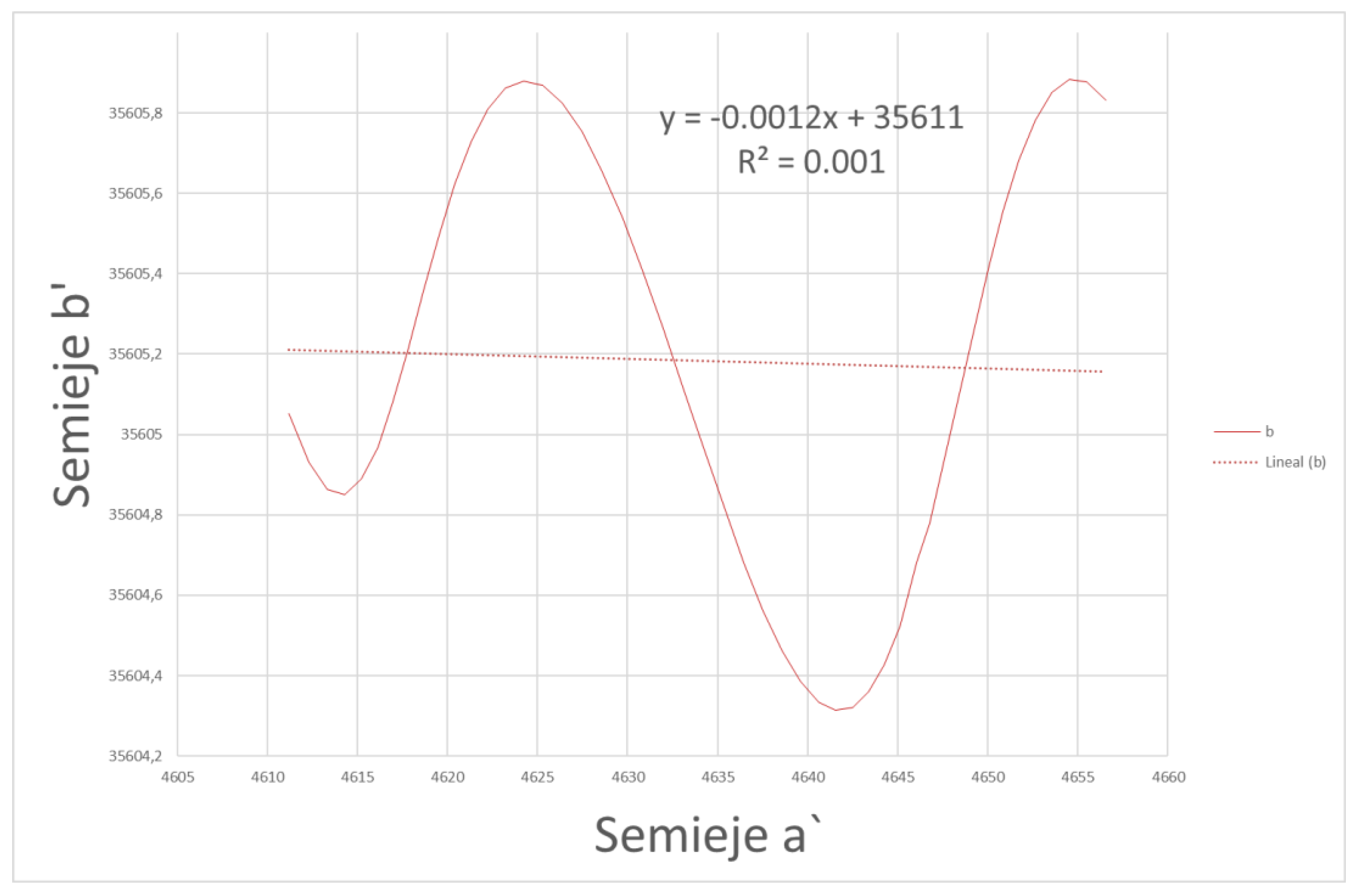
Where it can clearly be seen a pulsation on the fitted line. Reorienting the axes so that the straight line of the linear fit becomes the
x-axis results in a pulsation as
Figure 13 represents.
3.3. Prediction of Missing Positions
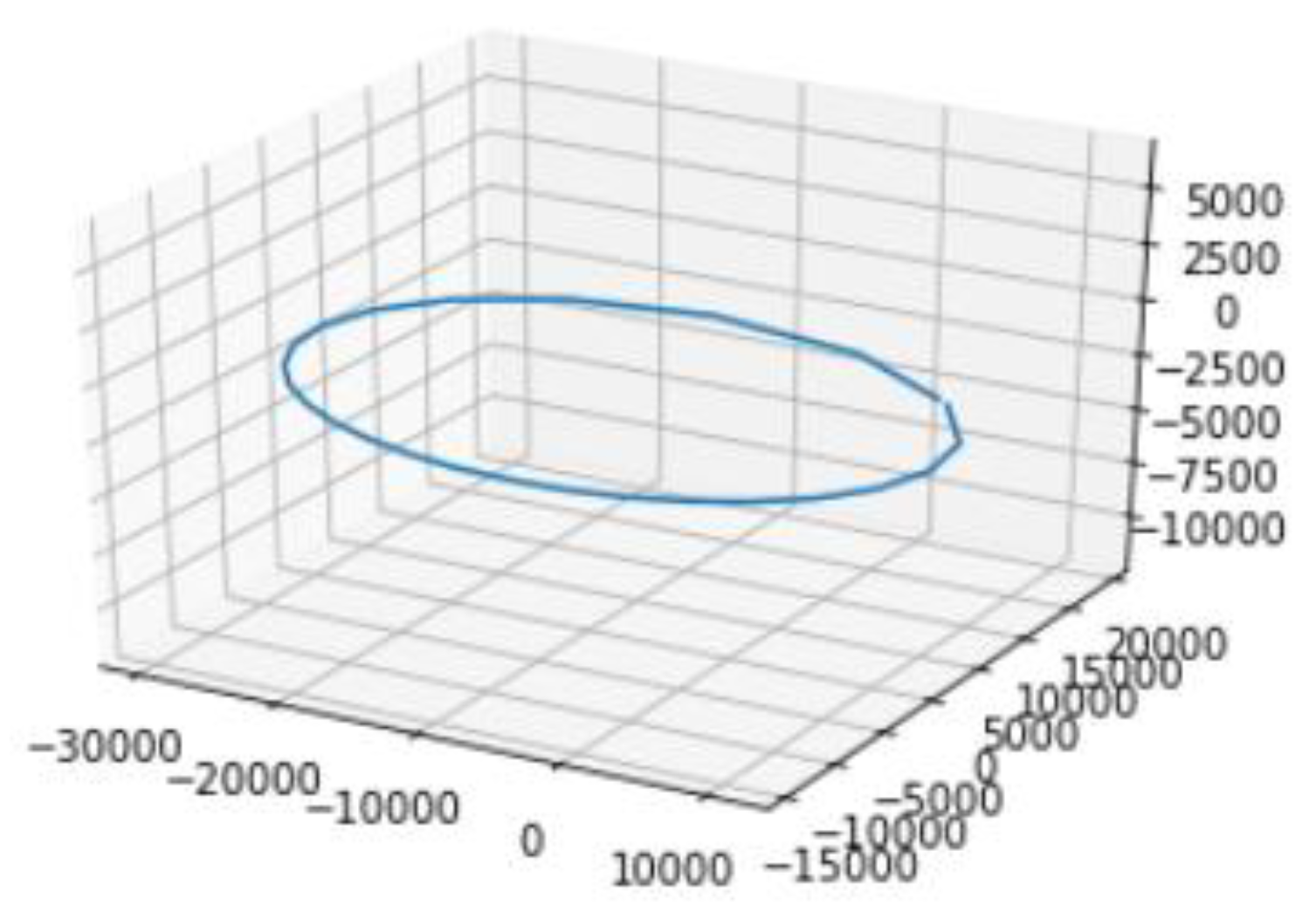
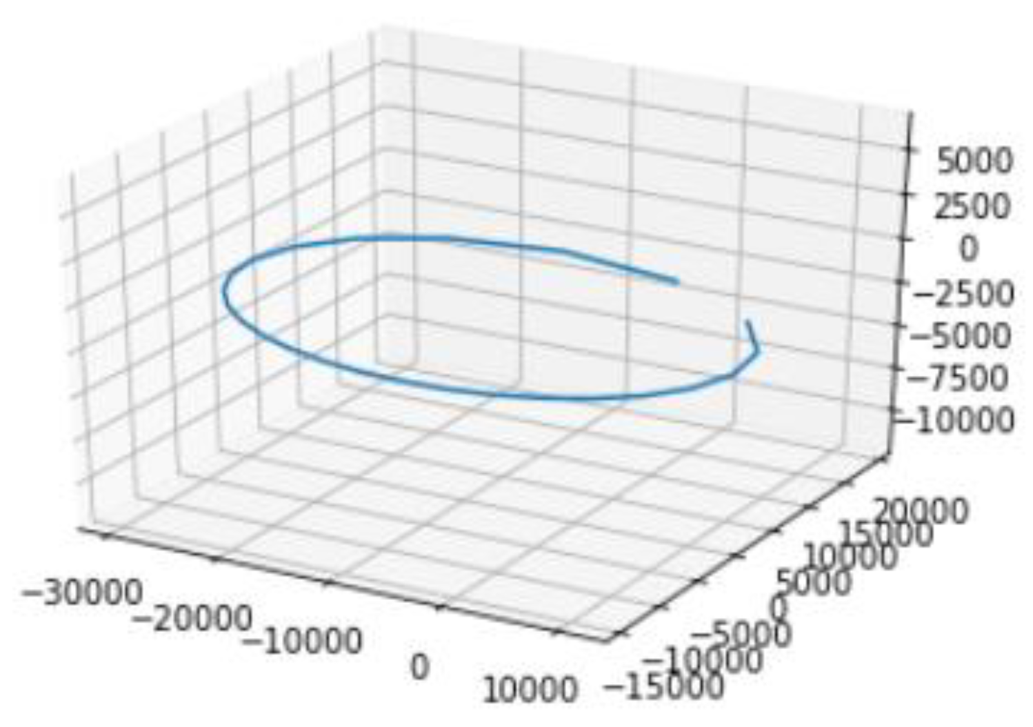
Among the data relating to the positions of the 600 satellites, we found that only 137 had uniform measurements made at 30-min intervals, which gave a degree of reliability to the results. The remaining 463 satellites had imprecise intervals, with gaps between measurements of different temporal sizes, which led to somewhat irregular orbit calculations on most occasions, and made the calculation of the estimated error of the satellite under study very imprecise, as seen in the orbit of
Figure 14, where there is no closing point, taking the next temporal measurement already in the course of the next orbit.
To solve this problem, a prediction has been made based on the historical measurements that allows to recreate smaller time windows, in this case of 1 min (the value of this parameter can be changed) in a uniform way. In this way, the closing of one orbit and the beginning of another can be estimated.
In this paper the use of median to estimate the different positions in each satellite dimension has been evaluated. The approach for the prediction exploits the pairs of time consecutive positions. The pseudocode is detailed as follows:
for each satellite:
-- for each measurement and its next
-- -- if the difference between the timestamps is greater than 2 min
-- -- -- calculate median between timestamps
-- -- -- for each dimension (x, y, z)
-- -- -- -- calculate the median between the positions
-- -- -- add estimated measure
The complexity of the algorithm is linear as a function of the number of measurements, except when there are missing measurements, where a prediction must be made about the missing measurements, with the complexity increasing the greater the number of missing gaps between the data.
In any case, when extrapolating it to the 600 satellites, the complexity will be a function of n2 (being n the number of elements) as seen in the source code shared (), with a computational time of less than one minute for all satellites during one month.
This technique is able to give accurate estimates the more times it is applied to fill in the gaps of missing measurements. The application of the repeated median method is better than the single median.
Using this method, we can extrapolate a more reliable approximation of the orbit described by the satellite, as shown in
Figure 15. Thus, the calculation of the error between the different orbits corresponding to the 26 days in the same satellite will be more accurate as shown in the following section.
3.4. Error Aproximation in Each Approximation and Comparison
While the a-axis seems to remain constant, in its drift the ellipse pulses on its semi-axis b, possibly due to corrections of the orbit.
The satellite seems to travel on a trajectory as represented on
Figure 16.
As the period of time over which it has been analyzed is 26 days, it seems that every 12 h it completes a cycle, and every 6 days or so its semi-axis has gone from maximum to minimum or vice versa.
As demonstrated, the trajectory of the satellite is clearly captured in an elliptical shape whose parameters, center and semi-axis can be calculated relatively easily from objective measurements.
When analyzing the evolution of these parameters, it is surprising that they do not remain constant over time, as might have been thought at first, but rather vary.
The center and the semi-major axis do remain constant, while the semi-minor axis oscillates sinusoidally in a stable manner. This leads to the conclusion that such changes are intentional and therefore predictable, they cannot be considered a measurement error. The center and the semi-major axis do remain constant, while the semi-minor axis oscillates sinusoidally in a stable manner. This leads to the conclusion that such changes are intentional and therefore predictable, they cannot be considered a measurement error. If this variation were taken as a rectangular distribution, such an error would give a conservative contribution of about 1.626/root(3) km, somewhat less than 0.94 km.
However, if the least squares fit with learning is used, we can approximate the position with 1.569/root(12) km, which is about 0.45 km standard deviation.
Consequently, the error in the position decreases and the error security is twice as high in the case of the adjustment compared to the raw prediction data.
The position of the satellite is predicted twice as reliably when the least squares adjustment is performed.
Analyzing the variation between the maximum value of the semi-axis b versus a, it turns out to be, in each method, 1569 km in the least squares method compared with the 1626 km as seen in
Table 2.
Therefore, the mathematical method proposed in this paper is sufficiently accurate for satellite trajectory prediction and estimation, taking into account the safety space maintained around each satellite.
4. Conclusions
As the number of satellites and spatial objects is growing exponentially, the amount of debris is increasing in the same proportion. This provokes a huge long term problem that must be controlled by providing reliable prediction methods to estimate the position of an object in space at a given time. In this paper, we have analyzed a set of data belonging to 600 satellites for 26 days. According to this information, we noticed some inconsistencies in the measurement intervals, for which we have presented a prediction algorithm that allows us to correct these inconsistencies and allows us to calculate an estimation of the satellite position in the future with higher reliability. With this prediction, we have estimated an error and limited the maximum error we can have in the prediction. It allows us to know the current position of the satellite, to predict the final position with a bounded error, and as new positions are acquired, the result can be updated.
As a general evaluation, the pros of this paper are the rigorous study that we have performed to predict new information in base to the data that we had with a high accuracy level, limiting the error in such prediction. Otherwise, we have applied a method that works and is able to locate the position of an object in a given time with a low margin of error. On the other hand, we have still work to do as we still have a lack of information to provide a statistical study as not all the information of the satellites was uniform, so it makes this process more complex. One key point can be the information related to the velocity of the object. In this study, we have not used this information but for future work, we will add this information to try to improve the positional error estimation despite being less than 2 km in both methods, which demonstrates the accuracy of the estimation.


