Social Network Optimization for WSN Routing: Analysis on Problem Codification Techniques

 ,
,  ,
,  ,
,  and
and
Abstract
1. Introduction
2. Swarm Intelligence
2.1. Particle Swarm Optimization
- Inertia: ‘I continue on my way’.
- Influence of the past: ‘I’ve always done in this way’.
- Influence by society: ‘If it worked for them, it would also work for me’.
2.2. Social Network Optimization
3. Wireless Sensor Network
3.1. Network Energy Model
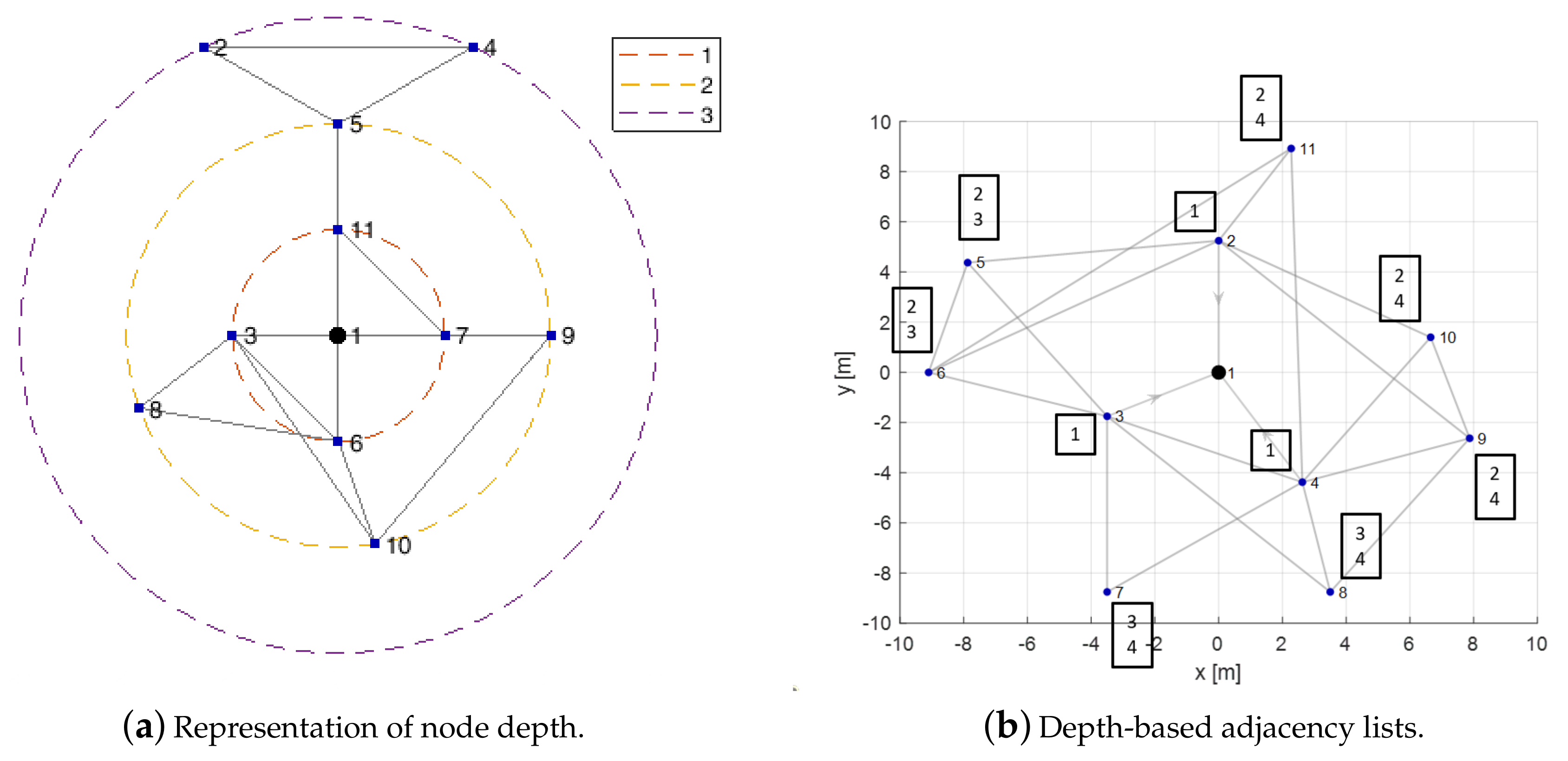
3.2. Problem Codification
3.3. Performance Calculation
3.4. Optimization Environment
4. Results and Discussion
4.1. Test Cases
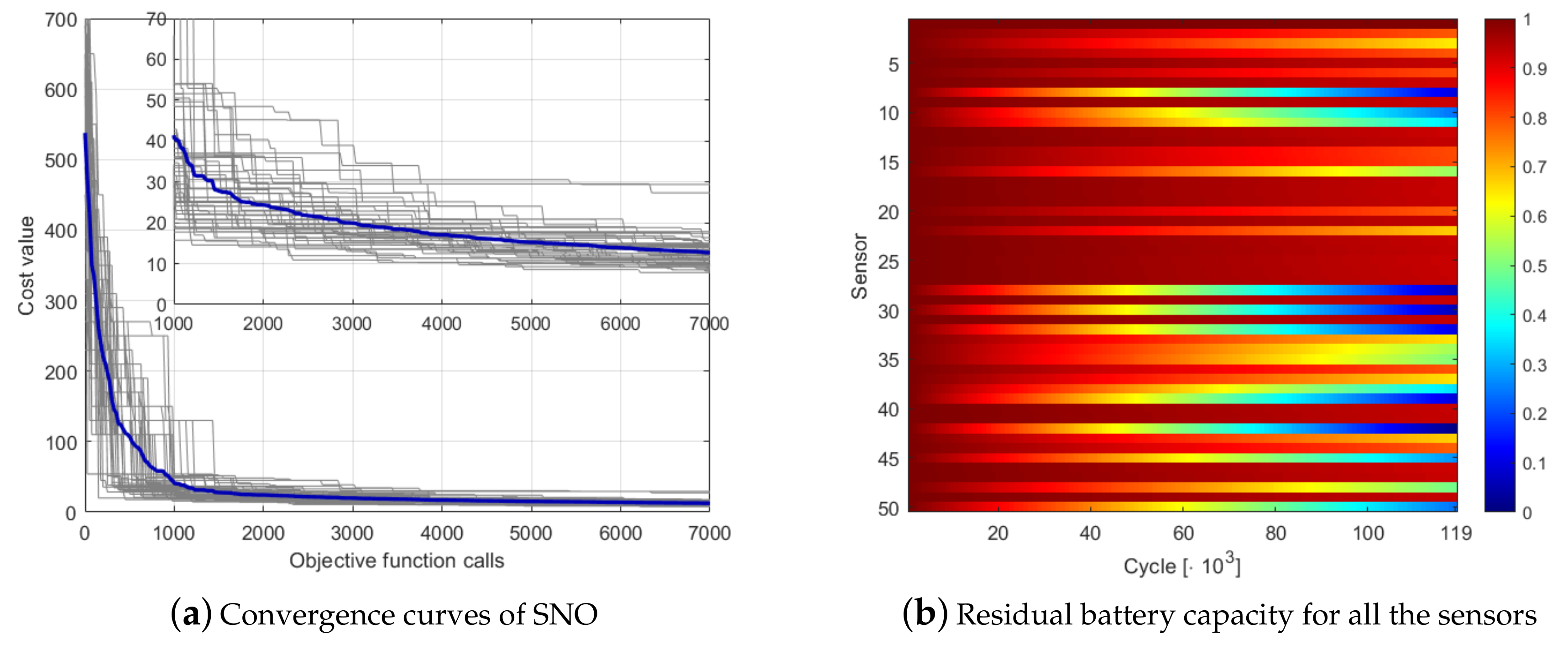
4.2. Results
4.3. Analysis of a Peculiar Case
5. Conclusions
Author Contributions
Funding
Conflicts of Interest
Abbreviations
| WSN | Wireless Sensor Network |
| KCC | Kilo Clock Cycles |
| SNO | Social Network Optimization |
| PSO | Particle Swarm Optimization |
References
- Buratti, C.; Conti, A.; Dardari, D.; Verdone, R. An overview on wireless sensor networks technology and evolution. Sensors 2009, 9, 6869–6896. [Google Scholar] [CrossRef] [PubMed]
- Iacca, G.; Neri, F.; Caraffini, F.; Suganthan, P.N. A differential evolution framework with ensemble of parameters and strategies and pool of local search algorithms. In European Conference on the Applications of Evolutionary Computation; Springer: Berlin, Germany, 2014; pp. 615–626. [Google Scholar]
- Grimaccia, F.; Gruosso, G.; Mussetta, M.; Niccolai, A.; Zich, R.E. Design of tubular permanent magnet generators for vehicle energy harvesting by means of social network optimization. IEEE Trans. Ind. Electron. 2017, 65, 1884–1892. [Google Scholar] [CrossRef]
- Hassan, R.; Cohanim, B.; De Weck, O.; Venter, G. A comparison of particle swarm optimization and the genetic algorithm. In Proceedings of the 46th AIAA/ASME/ASCE/AHS/ASC Structures, Structural Dynamics and Materials Conference, Austin, TX, USA, 18–21 April 2005; p. 1897. [Google Scholar]
- Baioletti, M.; Milani, A.; Poggioni, V.; Rossi, F. An ACO approach to planning. In European Conference on Evolutionary Computation in Combinatorial Optimization; Springer: Berlin, Germany, 2009; pp. 73–84. [Google Scholar]
- Caraffini, F.; Neri, F.; Poikolainen, I. Micro-differential evolution with extra moves along the axes. In Proceedings of the 2013 IEEE Symposium on Differential Evolution (SDE), Singapore, Singapore, 16–19 April 2013; pp. 46–53. [Google Scholar]
- Caraffini, F.; Kononova, A.V.; Corne, D. Infeasibility and structural bias in differential evolution. Inf. Sci. 2019, 496, 161–179. [Google Scholar] [CrossRef]
- Piotrowski, A.P. Review of differential evolution population size. Swarm Evol. Comput. 2017, 32, 1–24. [Google Scholar] [CrossRef]
- Baioletti, M.; Milani, A.; Santucci, V. Automatic algebraic evolutionary algorithms. In Italian Workshop on Artificial Life and Evolutionary Computation; Springer: Berlin, Germany, 2017; pp. 271–283. [Google Scholar]
- Baioletti, M.; Bari, G.D.; Milani, A.; Poggioni, V. Differential Evolution for Neural Networks Optimization. Mathematics 2020, 8, 69. [Google Scholar] [CrossRef]
- Simon, D. Biogeography-based optimization. IEEE Trans. Evol. Comput. 2008, 12, 702–713. [Google Scholar] [CrossRef]
- Sandeep, D.; Kumar, V. Review on clustering, coverage and connectivity in underwater wireless sensor networks: A communication techniques perspective. IEEE Access 2017, 5, 11176–11199. [Google Scholar] [CrossRef]
- Kuila, P.; Jana, P.K. A novel differential evolution based clustering algorithm for wireless sensor networks. Appl. Soft Comput. 2014, 25, 414–425. [Google Scholar] [CrossRef]
- Zahedi, Z.M.; Akbari, R.; Shokouhifar, M.; Safaei, F.; Jalali, A. Swarm intelligence based fuzzy routing protocol for clustered wireless sensor networks. Expert Syst. Appl. 2016, 55, 313–328. [Google Scholar] [CrossRef]
- Chen, Y.; Li, D.; Ma, P. Implementation of Multi-objective Evolutionary Algorithm for Task Scheduling in Heterogeneous Distributed Systems. JSW 2012, 7, 1367–1374. [Google Scholar] [CrossRef]
- Page, A.J.; Keane, T.M.; Naughton, T.J. Multi-heuristic dynamic task allocation using genetic algorithms in a heterogeneous distributed system. J. Parallel Distrib. Comput. 2010, 70, 758–766. [Google Scholar] [CrossRef] [PubMed]
- Ferjani, A.A.; Liouane, N.; Kacem, I. Task allocation for wireless sensor network using logic gate-based evolutionary algorithm. In Proceedings of the 2016 International Conference on Control, Decision and Information Technologies (CoDIT), St. Julian’s, Malta, 6–8 April 2016; pp. 654–658. [Google Scholar]
- Niccolai, A.; Grimaccia, F.; Mussetta, M.; Zich, R. Optimal Task Allocation in Wireless Sensor Networks by Means of Social Network Optimization. Mathematics 2019, 7, 315. [Google Scholar] [CrossRef]
- Ho, J.H.; Shih, H.C.; Liao, B.Y.; Chu, S.C. A ladder diffusion algorithm using ant colony optimization for wireless sensor networks. Inf. Sci. 2012, 192, 204–212. [Google Scholar] [CrossRef]
- Zhang, H.; Li, Z.; Shu, W.; Chou, J. Ant colony optimization algorithm based on mobile sink data collection in industrial wireless sensor networks. EURASIP J. Wirel. Commun. Netw. 2019, 2019, 152. [Google Scholar] [CrossRef]
- Hu, X.M.; Zhang, J.; Yu, Y.; Chung, H.S.H.; Li, Y.L.; Shi, Y.H.; Luo, X.N. Hybrid genetic algorithm using a forward encoding scheme for lifetime maximization of wireless sensor networks. IEEE Trans. Evol. Comput. 2010, 14, 766–781. [Google Scholar] [CrossRef]
- Caputo, D.; Grimaccia, F.; Mussetta, M.; Zich, R.E. An enhanced GSO technique for wireless sensor networks optimization. In Proceedings of the IEEE Congress on Evolutionary Computation, Hong Kong, China, 1–6 June 2008; pp. 4074–4079. [Google Scholar]
- Caputo, D.; Grimaccia, F.; Mussetta, M.; Zich, R.E. Genetical swarm optimization of multihop routes in wireless sensor networks. Appl. Comput. Intell. Soft Comput. 2010, 2010, 523943. [Google Scholar] [CrossRef]
- Omidvar, A.; Mohammadi, K. Particle swarm optimization in intelligent routing of delay-tolerant network routing. EURASIP J. Wirel. Commun. Netw. 2014, 2014, 147. [Google Scholar] [CrossRef]
- Poli, R.; Kennedy, J.; Blackwell, T. Particle swarm optimization. Swarm Intell. 2007, 1, 33–57. [Google Scholar] [CrossRef]
- Simon, D. Evolutionary Optimization Algorithms; John Wiley & Sons: Hoboken, NJ, USA, 2013. [Google Scholar]
- Engelbrecht, A. Particle swarm optimization: Velocity initialization. In Proceedings of the 2012 IEEE Congress on Evolutionary Computation, Brisbane, QLD, Australia, 10–15 June 2012; pp. 1–8. [Google Scholar]
- Trelea, I.C. The particle swarm optimization algorithm: Convergence analysis and parameter selection. Inf. Process. Lett. 2003, 85, 317–325. [Google Scholar] [CrossRef]
- Niccolai, A.; Grimaccia, F.; Mussetta, M.; Pirinoli, P.; Bui, V.H.; Zich, R.E. Social network optimization for microwave circuits design. Prog. Electromagn. Res. 2015, 58, 51–60. [Google Scholar] [CrossRef]
- Niccolai, A.; Grimaccia, F.; Mussetta, M.; Zich, R. Modelling of interaction in swarm intelligence focused on particle swarm optimization and social networks optimization. Swarm Intell. 2018, 551–582. [Google Scholar]
- Grimaccia, F.; Mussetta, M.; Niccolai, A.; Zich, R.E. Optimal computational distribution of social network optimization in wireless sensor networks. In Proceedings of the 2018 IEEE Congress on Evolutionary Computation (CEC), Rio de Janeiro, Brazil, 8–13 July 2018; pp. 1–7. [Google Scholar]
- Park, J.; Sahni, S. Maximum lifetime routing in wireless sensor networks. IEEE/ACM Trans. Netw. 2004, 12, 609–619. [Google Scholar]
- Dong, Q. Maximizing system lifetime in wireless sensor networks. In Proceedings of the IPSN 2005. Fourth International Symposium on Information Processing in Sensor Networks, Boise, ID, USA, 15 April 2005; pp. 13–19. [Google Scholar]
- Wong, J.Y.; Sharma, S.; Rangaiah, G. Design of shell-and-tube heat exchangers for multiple objectives using elitist non-dominated sorting genetic algorithm with termination criteria. Appl. Therm. Eng. 2016, 93, 888–899. [Google Scholar] [CrossRef]
- Eiben, A.E.; Smith, J.E. Introduction to Evolutionary Computing; Springer: Berlin, Germany, 2003; Volume 53. [Google Scholar]


| Parameter | Symbol | Value | Parameter | Symbol | Value |
|---|---|---|---|---|---|
| ine Communication package size | 100 bit | Communication energy | 5 pJ/b | ||
| Stored energy | 9 kJ | Amplification energy | 0.01 pJ/b |
| Number | Maximum | Number | Number of Adjacency-Based | Number of Depth-Based |
|---|---|---|---|---|
| of nodes | node depth | of connections | configurations | configurations |
| ine 20 | 4 | 54 | 1.51 | 192 |
| 25 | 4 | 102 | 1.08 | 2.4 |
| 30 | 3 | 157 | 4.3 | 1.63 |
| 35 | 4 | 143 | 4.36 | 8.82 |
| 40 | 4 | 192 | 4.44 | 4.12 |
| 45 | 4 | 226 | 3.87 | 2.93 |
| 50 | 5 | 253 | 4.64 | 4.46 |
| 55 | 6 | 314 | 4.8 | 9.63 |
| 60 | 4 | 341 | 3 | 7.1 |
| 65 | 6 | 250 | 2.17 | 1.59 |
| 70 | 7 | 215 | 1.6 | 9.78 |
| 75 | 4 | 547 | 7.94 | 8.8 |
| 80 | 5 | 549 | 2 | 1.16 |
| 85 | 7 | 410 | 2.22 | 1.29 |
| 90 | 5 | 650 | 1.95 | 1.33 |
| 95 | 6 | 501 | 2.08 | 3.58 |
| 100 | 5 | 792 | 2.96 | 2.61 |
| 105 | 4 | 831 | 3.51 | 1.92 |
| 110 | 6 | 506 | 2.02 | 4.79 |
| 115 | 5 | 987 | 2.64 | 1.52 |
| 120 | 8 | 436 | 7.5 | 8.62 |
| 125 | 4 | 1129 | 3.7 | 9.16 |
| 130 | 5 | 1000 | 6.63 | 4.62 |
| 135 | 8 | 581 | 1.23 | 4.45 |
| 140 | 5 | 1423 | 1.68 | 3.93 |
| 145 | 5 | 1459 | 3.27 | 2.83 |
| 150 | 8 | 784 | 2.5 | 5.38 |
© 2020 by the authors. Licensee MDPI, Basel, Switzerland. This article is an open access article distributed under the terms and conditions of the Creative Commons Attribution (CC BY) license (http://creativecommons.org/licenses/by/4.0/).
Share and Cite
Niccolai, A.; Grimaccia, F.; Mussetta, M.; Gandelli, A.; Zich, R. Social Network Optimization for WSN Routing: Analysis on Problem Codification Techniques. Mathematics 2020, 8, 583. https://doi.org/10.3390/math8040583
Niccolai A, Grimaccia F, Mussetta M, Gandelli A, Zich R. Social Network Optimization for WSN Routing: Analysis on Problem Codification Techniques. Mathematics. 2020; 8(4):583. https://doi.org/10.3390/math8040583
Chicago/Turabian StyleNiccolai, Alessandro, Francesco Grimaccia, Marco Mussetta, Alessandro Gandelli, and Riccardo Zich. 2020. "Social Network Optimization for WSN Routing: Analysis on Problem Codification Techniques" Mathematics 8, no. 4: 583. https://doi.org/10.3390/math8040583
APA StyleNiccolai, A., Grimaccia, F., Mussetta, M., Gandelli, A., & Zich, R. (2020). Social Network Optimization for WSN Routing: Analysis on Problem Codification Techniques. Mathematics, 8(4), 583. https://doi.org/10.3390/math8040583