Article

A New One-Parameter Model Supports an Upside-Down Bathtub Failure Rate: Theory, Inference, and Real-World Applications

1
Department of Mathematical Sciences, College of Science, Princess Nourah Bint Abdulrahman University, P.O. Box 84428, Riyadh 11671, Saudi Arabia
2
Faculty of Technology and Development, Zagazig University, Zagazig 44519, Egypt
*
Author to whom correspondence should be addressed.
Mathematics 2026, 14(9), 1566; https://doi.org/10.3390/math14091566
Submission received: 24 March 2026 / Revised: 30 April 2026 / Accepted: 2 May 2026 / Published: 6 May 2026
(This article belongs to the Special Issue Computational Statistics: Analysis and Applications for Mathematics)

Abstract

Researchers often develop ordinal hazard distributions, whether increasing or decreasing, into multi-parameter distributions to derive various forms of the hazard function. This process necessitates the formulation of a multi-parameter hazard function, which involves a more complex mathematical expression. In contrast, this study introduces a new one-parameter lifetime model, termed the Inverted Z–Lindley (IZL) distribution, which is capable of capturing an upside-down bathtub-shaped failure rate without sacrificing analytical simplicity. Fundamental distributional properties of the IZL model are rigorously established, including closed-form expressions for the probability density, cumulative distribution, reliability, and hazard rate functions. Theoretical analysis shows that the density is strictly positive, unimodal, positively skewed, and heavy-tailed, while the hazard rate is unimodal with vanishing limits at both extremes. Fractional moments are obtained, and the non-existence of classical moments is formally justified, motivating the use of quantile-based and inactivity-time reliability measures. Besides the quantile function, several key reliability measures, including the mean inactivity time and strong mean inactivity time functions, and order statistics, are also developed. Inferential procedures are constructed under Type-II censoring using both likelihood-based and Bayesian frameworks. The existence and uniqueness of the frequentist estimator are established, while Bayesian estimation is implemented via Markov chain Monte Carlo methods under informative gamma priors. Several interval estimation techniques—including asymptotic, bootstrap, Bayesian credible, and highest posterior density intervals—are developed and compared through extensive Monte Carlo simulations. The practical relevance of the proposed model is demonstrated using real datasets from environmental health and communication engineering, where the IZL distribution consistently outperforms fifteen well-established inverted lifetime models according to likelihood-based criteria, information measures, and goodness-of-fit diagnostics. Overall, the IZL model offers a powerful, interpretable, and computationally efficient alternative for modeling heavy-tailed lifetime data with non-monotone failure behavior, contributing meaningfully to modern distribution theory and applied reliability analysis.

1. Introduction

The Lindley distribution, originally introduced by Lindley [1], has emerged as a versatile and practical model in reliability analysis, survival studies, and applied probability. Its popularity stems from its simple yet flexible one-parameter structure, which allows it to effectively model lifetime and waiting-time data exhibiting skewness and nonmonotone hazard rates. Compared to classical distributions such as the exponential or gamma, the Lindley distribution often provides a superior fit for small to moderate sample sizes, offering enhanced interpretability and computational convenience; see Qayoom et al. [2] for additional details. Its applications span diverse fields, including engineering reliability, health sciences, actuarial studies, and queuing systems, highlighting its importance as a tool for modeling stochastic phenomena.
Despite its widespread application, the Lindley distribution is constrained by a monotonically decreasing hazard function, limiting its flexibility in capturing a range of lifetime behaviors. To address this limitation, a modern enhancement of the classical Lindley family, named the ZLindley distribution, has been introduced by Saaidia et al. [3] as a combination of exponential and gamma components, thereby extending the adaptability of traditional models like the Lindley distribution. This development expands upon the classical Lindley model by adding an additional linear term to its density expression, which enhances flexibility in modeling lifetime data characterized by varying hazard rate behaviors. Unlike the classical Lindley and other simple lifetime distributions, the ZLindley (ZL( α )) distribution exhibits improved adaptability in capturing a broad spectrum of hazard rate behaviors, including increasing and near-constant shapes, making it well-suited for heterogeneous reliability and survival data. Its statistical properties, such as closed-form expressions for the probability density and distribution functions, central tendency measures, and reliability characteristics, have been rigorously derived, facilitating both theoretical analysis and practical implementation. Empirical studies demonstrate that the ZL( α ) model often outperforms several classical competitors (e.g., Lindley, Weibull, Gamma) in goodness-of-fit for real datasets, underscoring its advantage in modeling over-dispersion and complex lifetime dynamics; see Alotaibi and Elshahhat [4].
A random variable X is said to follow the one-parameter ZL distribution (with α > 0 is a scale) if its probability density function (PDF), denoted by f ( · ; α ) , and corresponding cumulative distribution function (CDF), denoted by F ( · ; α ) , are given respectively by
f ( x ; α ) = α 2 ( 1 + α ) ( 1 + α ( 2 + x ) ) e α x , x > 0 ,
and
F ( x ; α ) = 1 1 + α x 2 ( 1 + α ) e α x ,
see, for more details, Mahnashi and Zaagan [5]. The inversion technique is a powerful approach in statistical modeling, developed by applying a reciprocal transformation to a positive random variable. This method produces inverted distributions with enhanced flexibility, allowing the generation of diverse hazard rate behaviors, including upside-down bathtub (inverted-bathtub) shapes, which is particularly valuable for systems exhibiting high early risk followed by stabilization. Inverted distributions often provide superior fits for real-world data compared to classical lifetime models, especially in contexts where large survival times, low failure rates, or extreme events are prevalent; see Sharma et al. [6], Nguyen et al. [7], Tomer and Panwar [8], Choudhary et al. [9], Alqasem et al. [10], and Singh et al. [11], among others.
Classical one-parameter lifetime models are attractive because of their simplicity and easy interpretation. However, they often become inadequate when observed hazard rates are non-monotone. Many practical systems exhibit an upside-down bathtub (UBT) hazard shape, where failure risk first increases and then decreases. Such behavior cannot be captured well by exponential, Lindley, or other monotone one-parameter models. One important example arises in communication engineering systems such as sensors, wireless nodes, and transceivers. These devices may suffer early failures due to calibration errors, manufacturing defects, or installation stress before becoming stable later. Another example occurs in environmental health after exposure to pollutants, radiation, or toxic chemicals. In such cases, health risk may initially rise and then decline because of adaptation, treatment, or removal of highly susceptible individuals. Similar patterns also appear in industrial units exposed to transient overload or frictional adjustment during early operation. These practical limitations motivate the proposed inverted ZLindley (IZL) model as a parsimonious one-parameter model with UBT hazard flexibility.
In the next section, we introduce the IZL model that preserves analytical simplicity while substantially enriching hazard-rate behavior. The main objectives of the current study can be summarized fourfold as follows:
  • A new IZL model is proposed, providing a flexible distributional form capable of capturing UBT failure rate behavior while retaining the simplicity of a single-parameter structure. The probability density and hazard rate functions are analytically shown to be strictly positive, unimodal, and heavy-tailed, with the hazard rate exhibiting a UBT shape—an essential feature for modeling early-risk-dominated systems.
  • Parameter estimation is developed under Type-II censored samples (T2CSs), including existence and uniqueness of the maximum likelihood, Bayesian estimation with informative gamma prior, and implementation via MCMC methods. Six interval estimation approaches are proposed and compared, including asymptotic, bootstrap, Bayesian credible, and HPD intervals, providing a comprehensive inferential toolkit.
  • Comprehensive simulations assess estimator accuracy, bias, interval length, and coverage probability, demonstrating the superior finite-sample performance of Bayesian and HPD-based procedures, particularly under censoring.
  • The adaptability of the proposed IZL distribution is demonstrated through two real datasets drawn from environmental health and communication engineering, both of which naturally exhibit heavy-tailed behavior, positive skewness, and non-monotone failure dynamics. These features are difficult to capture simultaneously using existing inverted lifetime models. To rigorously assess adequacy, the IZL model is benchmarked against 15 well-established inverted distributions using likelihood-based, information-theoretic, and goodness-of-fit criteria. Across both applications, the IZL model consistently emerges as the most competitive compared to inverted Lindley, inverted X-Lindley, inverted gamma, inverted Weibull, inverted Chen, and inverted Nadarajah–Haghighi, among others.
The rest of this work is classified as follows: Section 2 introduces the proposed IZL model and presents its fundamental definitions. Section 3 derives key statistical and reliability properties. In Section 4 and Section 5, several point and interval parameter estimation procedures are investigated, respectively. The simulation design of the estimators is done in Section 6. Two real data applications from communication engineering and environmental health are analyzed in Section 7. Finally, Section 8 provides the concluding remarks and future research directions.

2. The Inverted ZLindley Distribution

This section presents the fundamental analytical characteristics of the IZL distribution, covering its principal functions, including the CDF, PDF, reliability function, hazard (failure) rate function, and related measures.

2.1. Main Distribution Functions

Now, let Y be a random variable that follows the ZL distribution with the CDF F ( · ) , in (1), and with the PDF f ( · ) , in (2). Taking Y = X 1 , the random variable Y will follow the IZL model, symbolized as Y I Z L ( α ) , with the following CDF (say, F ( · ) ) and PDF (say,  f ( · ) ):
F ( y ; α ) = 1 + α 2 ( 1 + α ) y e α / y , y > 0 ,
and
f ( y ; α ) = α 2 ( 1 + α ) y 2 1 + 2 α + α y e α / y , y > 0 .
For more specification, in Appendix A, we establish the mathematical soundness of the proposed distribution by verifying that the CDF (3) satisfies all fundamental properties required of a valid distribution function.

2.2. Reliability and Failure Rate

The survival (reliability) function and the hazard rate, also referred to as the failure rate function (FRF) (at a mission time point t > 0 ), corresponding to the IZL distribution are given, respectively, by
R ( t ; α ) = 1 1 + α 2 ( 1 + α ) t e α t , t > 0 ,
and
h ( t ; α ) = α 1 + 2 α + α t 2 ( 1 + α ) t 2 ( e α t 1 ) α t , t > 0 .
Theorem 1.
Let X IZL ( α ) with α > 0 . Then the probability density function f ( y ; α ) is strictly positive on ( 0 , ) and vanishes at both endpoints, that is,
lim y 0 + f ( y ; α ) = 0 and lim y f ( y ; α ) = 0 .
Moreover, f ( y ; α ) is unimodal with a unique global maximum; it increases from zero to its mode and decreases thereafter, exhibiting positive skewness and a heavy right tail with polynomial decay of order O ( y 2 ) as y .
In contrast, the hazard rate function h ( y ; α ) of the IZL distribution is continuous and strictly positive for all y > 0 , vanishes at the boundaries,
lim y 0 + h ( y ; α ) = 0 and lim y h ( y ; α ) = 0 ,
and is unimodal with a UBT shape. Specifically, h ( y ; α ) increases from zero to a finite maximum and then decreases monotonically back to zero as y .
Proof. 
See Appendix B.    □
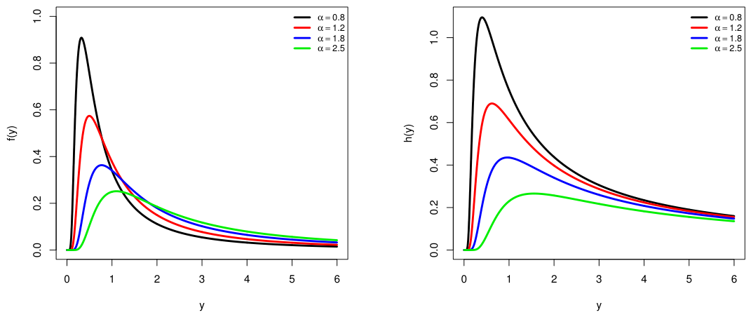
Figure 1 illustrates the shapes exhibited by the PDF and HRF of the IZL distribution for different values of α . Consistent with Theorem 1, the IZL density is strictly positive, unimodal, and positively skewed, with the tail becoming heavier as α increases.
Correspondingly, the HRF displays a characteristic UBT shape, rising from zero to a peak before gradually declining. These distinctive features offer notable practical advantages for modeling lifetime and reliability data: the unimodal density allows the IZL distribution to accurately capture phenomena with a single predominant mode and inherent positive skewness, while the flexible hazard rate effectively represents systems or components that experience an early increase in failure risk followed by a reduction, reflecting aging, stabilization, or burn-in effects. Overall, the combination of these shape properties enhances the interpretability, adaptability, and applicability of the IZL distribution in survival analysis and reliability studies, making it a versatile tool for capturing complex lifetime behaviors observed in real-world data.

2.3. Density Expansion

In this subsection, we derive an infinite series representation of the IZL density function to obtain a more tractable analytical form. This expansion facilitates the study of structural properties such as tail behavior and moment existence, and provides a convenient foundation for further theoretical developments. First, we expand the exponential term e α / y using its Maclaurin series. For any t > 0 , e t = k = 0 ( 1 ) k t k k ! . Setting t = α / y , we obtain
e α / y = k = 0 ( 1 ) k k ! α y k .
Substituting into the PDF (4) yields
f ( y ; α ) = 1 + 1 2 ( 1 + α ) y k = 0 ( 1 ) k k ! α y k + 2 .
From (8), we redistribute the polynomial term:
f ( y ; α ) = k = 0 ( 1 ) k k ! α y k + 2 + 1 2 ( 1 + α ) y k = 0 ( 1 ) k k ! α y k + 2 .
Simplifying powers of y in (9), we obtain
f ( y ; α ) = k = 0 ( 1 ) k α k + 2 k ! 1 y k + 2 + 1 2 ( 1 + α ) k = 0 ( 1 ) k α k + 2 k ! 1 y k + 3 .
Therefore, the IZL density admits the following infinite series representation:
f ( y ; α ) = k = 0 ( 1 ) k α k + 2 k ! y ( k + 2 ) + 1 2 ( 1 + α ) k = 0 ( 1 ) k α k + 2 k ! y ( k + 3 ) .
Equivalently, this may be written in compact form as
f ( y ; α ) = k = 0 ( 1 ) k α k + 2 k ! y ( k + 2 ) + 1 2 ( 1 + α ) y ( k + 3 ) .
This expansion expresses the IZL density as a weighted infinite linear combination of inverse power functions of y, which is particularly useful for deriving moments, studying tail behavior, and developing approximation results.

3. Statistical Properties

This section presents several properties of the IZL distribution, including moments, mean inactivity time, and order statistics, among others.

3.1. Quantile and Quartiles

This part introduces the quantile function and associated quartiles of the IZL model, which play a central role in understanding its distributional structure and spread. The quantile representation not only facilitates efficient random variate generation for simulation studies but also enables straightforward computation of median, quartiles, and other percentile-based measures.
Theorem 2.
Let Y be a random variable following the IZL(α) distribution, then, for 0 < u < 1 , the quantile function Q ( u ) = F 1 ( u ) exists in closed form and is given by
Q ( u ) = α W 1 2 ( 1 + α ) u e 2 ( 1 + α ) 2 ( 1 + α ) ,
where W 1 ( · ) denotes the negative branch of the Lambert W function. Consequently, the IZL distribution admits an explicit quantile representation, which is particularly useful for random variate generation and simulation-based inference.
Proof. 
See Appendix C.    □
If we let Y IZL ( α ) with α > 0 , by taking u = 0.25, 0.50, and 0.75, the first quartile ( Q 1 ), median ( Q 2 ), and third quartile ( Q 3 ) are obtained from the quantile function as follows:
Q 1 = α W 1 1 2 ( 1 + α ) e 2 ( 1 + α ) 2 ( 1 + α ) ,
Q 2 = α W 1 ( 1 + α ) e 2 ( 1 + α ) 2 ( 1 + α ) ,
and
Q 3 = α W 1 3 2 ( 1 + α ) e 2 ( 1 + α ) 2 ( 1 + α ) ,
where W 1 ( · ) denotes the negative branch of the Lambert W function.
Corollary 1.
Because the argument of the Lambert W function is negative, the appropriate branch ensuring Q ( u ) > 0 is the W 1 branch. Hence, the IZL distribution admits a closed-form quantile representation in terms of the Lambert W function, which facilitates random variate generation and simulation studies.
Corollary 2.
The ‘GoFKernel’ package (version 2.1-3), proposed by Pavia and Pavia [12], is recommended to generate random variates from the IZL distribution. In particular, using the quantile function given in Theorem 2, the first quartile, median, and third quartile of the IZL distribution can be obtained directly by setting u = 1 / 4 , u = 2 / 4 , and u = 3 / 4 , respectively.

3.2. The rth Ordinary Moment

Moments constitute fundamental descriptive measures in probability theory, as they summarize key characteristics of a distribution including central tendency, variability, and tail heaviness. In this subsection, we derive the general expression for the rth ordinary moment of the IZL distribution and establish the conditions under which it exists.
Theorem 3.
Let Y IZL ( α ) ; then for r < 1 , its rth moment is
E ( Y r ) = α r 2 ( 1 + α ) ( 1 + 2 α ) Γ ( 1 r ) + Γ ( 2 r ) , r < 1 .
Proof. 
See Appendix D.    □
Remark 1.
The divergence of the mean and variance is a direct consequence of the heavy right tail of the IZL distribution. Such behavior is common in inverse-type and heavy-tailed lifetime models, including the Cauchy and Lévy distributions, as well as the Pareto distribution under certain parameter settings. While classical moment-based summaries (e.g., mean and variance) are not defined, inference can rely on robust alternatives, such as median, quantiles, or fractional moments ( r < 1 ), which remain finite and provide meaningful measures.

3.3. Mean Residual Life

Mean residual life (MRL) evaluates the expected remaining lifetime of an item that has survived up to time t, providing valuable insight into the future reliability behavior of the distribution. It is an important tool in actuarial science and reliability tests because it helps characterize aging properties and supports maintenance or replacement decision-making.
Theorem 4.
Let Y IZL ( α ) ; the MRL ( · ) of Y is
MRL ( t ) = 1 R t E ( Y ) α 2 ( 1 + α ) ( 1 + 2 α ) E 1 α t + e α t t , t > 0 ,
where E 1 ( · ) denotes the exponential integral.
Proof. 
See Appendix E.    □
Corollary 3.
Since E ( Y ) = , it implies that the MRL ( t ) = , t > 0 . This property reflects the heavy-tailed nature of the IZL model, similar to other inverse-type and heavy-tailed lifetime distributions such as the Cauchy and Lévy families, where expectation-based reliability measures are not finite.

3.4. Mean Inactivity Time

The mean inactivity time (M-IT) function gives the expected time a system or component has been inactive or failed before a given time, reflecting how long it typically stays non-operational. Consider the quantity y Y | Y y , where Y is a lifetime random variable. The M-IT function of Y is given by
M I - T ( t ) = E ( t Y | Y t ) = 0 t F y d y F t .
Substituting the CDF (3) into the integral in (11) gives
0 t F ( y ) d y = 0 t e α / y d y + α 2 ( 1 + α ) 0 t e α / y y d y .
Use the substitution u = α / y , so that y = α / u and d y = α u 2 d u . Then, we get
0 t e α / y d y = α t e u α u 2 d u = α α t u 2 e u d u = α Γ 1 , α t .
Similarly, for 0 t y 1 e α / y d y , we have d y / y = d u / u , giving
0 t e α / y y d y = α t e u u ( d u ) = α t e u u d u = Ei α t ,
where Ei ( z ) is the exponential integral function.
Combining the two terms (13) and (14), Equation (12) becomes
0 t F ( y ) d y = α Γ 1 , α t + α 2 ( 1 + α ) Ei α t ,
where Γ ( s , z ) is the upper incomplete gamma function and Ei ( z ) is the exponential integral. Substituting (15) into (11), for t > 0 , the M-IT function of the IZL model can be easily obtained.

3.5. Strong Mean Inactivity Time

A strong mean inactivity time (SM-IT) function measures the expected remaining time until a system or component fails, given that it has already survived up to a certain time, with an emphasis on its monotone or stronger reliability properties. Its benefits include providing more sensitive insights into system aging and reliability behavior, helping in maintenance planning and replacement strategies (see Yang et al. [13]). The SM-IT of a lifetime r v Y is defined as
SMIT t = 1 F t 0 t 2 y F y d y .
If X I Z L ( α ) , from (3), we solve the integral term in (16) as follows:
0 t 2 y F ( y ) d y = 0 t 2 y + α 1 + α e α y d y .
Rearranging (17), we get
0 t 2 y F ( y ) d y = 0 t 2 y e α y d y + α 1 + α 0 t e α y d y .
Consider u = α y , which implies y = α / u and d y = α u 2 d u ; then
0 t 2 y e α y d y = 2 α 2 α t u 3 e u d u = 2 α 2 Γ 2 , α t ,
and
0 t e α y d y = α α t u 2 e u d u = α Γ 1 , α t .
Substituting (19) and (20) into (18), we obtain
0 t 2 y F ( y ) d y = 2 α 2 Γ 2 , α t + α 2 1 + α Γ 1 , α t .
As a result, the SM-IT of the IZL model is given by
SMIT ( t ) = 2 α 2 Γ 2 , α t + α 2 ( 1 + α ) 1 Γ 1 , α t 1 + α 2 ( 1 + α ) t e α t , t > 0 ,
where Γ ( s , z ) denotes the upper incomplete gamma function.

3.6. Order Statistics

Order statistics refer to the sorted values of a sample from smallest to largest. Their benefits include enabling estimation of population percentiles, studying extreme events, and supporting reliability, stress–strength, and extreme value analyses. Let Y 1 , Y 2 , , Y n be a random sample from the IZL distribution with PDF (4) and CDF (3). Suppose Y 1 : n Y 2 : n Y n : n denote the order statistics of a random sample of size n drawn from the IZL population. The CDF and PDF of Y m : n for m = 1 , 2 , , n (denoted by f m : n ( y ) and F m : n ( y ) ) are given by
F Y m : n ( y ) = k = m n n k F ( y ; α ) k 1 F ( y ; α ) n k .
and
f Y m : n ( y ) = F ( y ; α ) m 1 1 F ( y ; α ) n m f ( y ; α ) ,
respectively, where m = n ! ( m 1 ) ! ( n m ) ! .
Using the binomial expansion theorem, the CDF and PDF of the m-th order statistic can be expanded as follows:
F Y m : n ( y ) = k = m n n k F ( y ; α ) k 1 F ( y ; α ) n k = k = m n n k F ( y ; α ) k j = 0 n k n k j ( 1 ) j F ( y ; α ) j = k = m n j = 0 n k n k n k j ( 1 ) j F ( y ; α ) k + j ,
and
f Y m : n ( y ) = m F ( y ; α ) m 1 1 F ( y ; α ) n m f ( y ; α ) = m F ( y ; α ) m 1 f ( y ; α ) j = 0 n m n m j ( 1 ) j F ( y ; α ) j = m f ( y ; α ) j = 0 n m n m j ( 1 ) j F ( y ; α ) m 1 + j ,
respectively.
Substituting the CDF (3) and PDF (4) into (25) and (26), the CDF and PDF of the m-th order statistics will be
F Y m : n ( y ) = k = m n j = 0 n k n k n k j ( 1 ) j 1 + α 2 ( 1 + α ) y e α / y k + j ,
and
f Y m : n ( y ) = m α 2 ( 1 + α ) y 2 1 + 2 α + α y e α / y × j = 0 n m n m j ( 1 ) j 1 + α 2 ( 1 + α ) y e α / y m 1 + j ,
respectively. As special cases, the smallest and largest order statistics, Y 1 : n and Y n : n , respectively, are given by
  • For the minimum, Y 1 : n , the CDF simplifies to
    F Y 1 : n ( y ) = 1 1 1 + α 2 ( 1 + α ) y e α / y n ,
    and the PDF is
    f Y 1 : n ( y ) = n α 2 ( 1 + α ) y 2 1 + 2 α + α y e α / y 1 1 + α 2 ( 1 + α ) y e α / y n 1 .
  • For the maximum, Y n : n , the CDF is
    F Y n : n ( y ) = 1 + α 2 ( 1 + α ) y e α / y n ,
    and the PDF is
    f Y n : n ( y ) = n α 2 ( 1 + α ) y 2 1 + 2 α + α y e α / y 1 + α 2 ( 1 + α ) y e α / y n 1 .
The explicit forms of the general, minimum, and maximum order IZL statistics are suitable for reliability analysis, extreme value modeling, and numerical computation of probabilities.

4. Parameter Estimation

This section addresses both likelihood-based and Bayesian inferential procedures under a T2CS, with the objective of constructing point and interval estimators for the IZL parameter.

4.1. Likelihood Inference

Let y = ( Y 1 : n , Y 2 : n , , Y j : n ) , with j < n , denote a T2CS consisting of the first j observed failure times from a life test conducted on n independent units, all initiated at time zero. The joint likelihood function (LF) of the observed order statistics Y i : n for i = 1 , 2 , , j , denoted by L ( · ) , is then given by
L ( y | α ) = j i = 1 j f ( y i : n ; α ) 1 F ( y j : n ; α ) n j ,
where j = n ! ( n j ) ! . Substituting (4) and (3) into (32), we express the LF and log-LF as follows:
L ( y α ) α j ( 1 + α ) j i = 1 j 1 + 2 α + α y i : n e α i = 1 j y i : n 1 1 1 + ϑ j e α y j : n n j
and
log L ( y α ) j α 1 + α + i = 1 j log 1 + 2 α + α y i : n α i = 1 j y i : n 1 + ( n j ) log 1 1 + ϑ j e α / y j : n ,
respectively, where ϑ j = α 2 ( 1 + α ) y j : n .
Differentiating (34) with respect to α , the score function of α (say, U ( α ) ) becomes
U ( α ) = j α j 1 + α + i = 1 j 2 + y i : n 1 1 + 2 α + α y i : n 1 i = 1 j y i : n 1 ( n j ) e α / y j : n ( α ( 1 + α ) ) 1 ϑ j y j : n 1 1 + ϑ j 1 1 + ϑ j e α / y j : n .
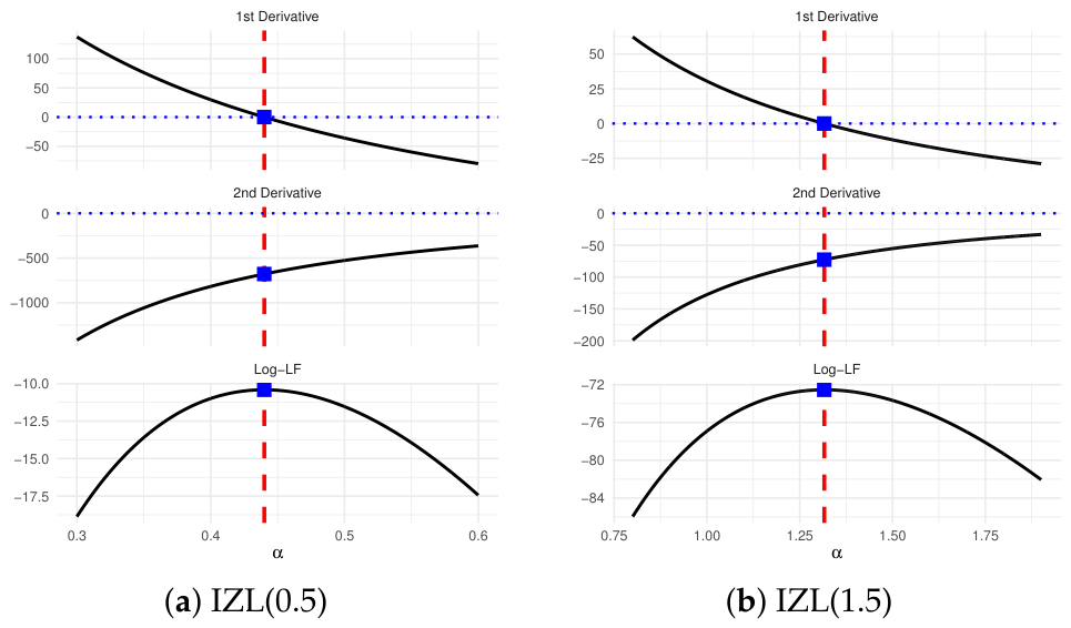
Since the score equation U ( α ) = 0 in (35) does not admit a closed-form solution, the maximum likelihood estimator (MLE) of α (denoted by α ^ ) must be obtained numerically using iterative methods such as Newton–Raphson (NR). To achieve this goal, the maxLik package in R (version 4.2.2), developed by Henningsen and Toomet [14], is recommended for this purpose. Using a T2CS dataset with ( n , j ) = ( 100 , 50 ) drawn from the IZL ( 0.5 ) and IZL ( 1.5 ) distributions, Figure 2 depicts the log-LF and its first and second derivatives with respect to α . The log-LF curve is strictly concave over the admissible parameter space α > 0 and exhibits a single interior maximum, providing clear empirical evidence for the existence of the MLE of α .
Moreover, the score function crosses the horizontal axis exactly once, implying that the normal equation U ( α ) = 0 admits a unique solution. At this same point, the second derivative of the log-LF is strictly negative, confirming that the stationary point corresponds to a local maximum rather than a minimum or saddle point. Since the log-LF is smooth and unimodal on α > 0 , this local maximum is also the global maximum. Consequently, the MLE of α exists and is unique, which guarantees the numerical stability and convergence of the recommended NR iterative optimization algorithm.

4.2. Bayesian Inference

This subsection considers the Bayesian estimation of the parameter α . A gamma conjugate prior is employed for α due to its flexibility in shape as determined by the hyperparameters ( ε 1 , ε 2 ) , which allows it to accommodate a wide range of prior beliefs while ensuring proper support on the positive real line; see [15] for further details. Let the prior for α be
π ( α ) α ε 1 1 e ε 2 α , ε 1 , ε 2 > 0 , α > 0 .
Then, the posterior probability density function of α , denoted by Π ( α y ) , is obtained as
Π ( α y ) L ( y α ) × π ( α ) ,
which combines the information from the observed data y with the gamma prior to yield the posterior distribution for α as follows:
Π ( α y ) = C 1 α j + ε 1 1 ( 1 + α ) j i = 1 j 1 + 2 α + α y i : n e α ε 2 + i = 1 j y i : n 1 1 1 + ϑ j e α y j : n n j ,
where C = 0 L ( y α ) × π ( α ) d α denotes the normalizing term.
As a result, the Bayes estimator of α , denoted α ˜ , and β ˜ , under the squared error loss (SEL), are directly given by the posterior expectation of α , as follows:
α ˜ = C 1 0 α · Π α d α .
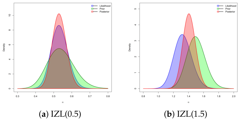
Due to the nonlinear form of the posterior mean in (39), the posterior density of α cannot be expressed in closed form. Consequently, a Markov chain Monte Carlo (MCMC) approach is recommended to generate posterior samples from (38), allowing the evaluation of Bayes estimators of α and the construction of ( 1 a ) 100 % BCI and HPD intervals. Since the posterior PDF of α does not correspond to any standard distribution, MCMC sampling is required. Using the same T2CS dataset illustrated in Figure 2, Figure 3 displays the prior π ( α ) , the likelihood L ( · ) , and the posterior Π ( · ) . These plots indicate that the posterior distributions of α are approximately symmetric and roughly normal. Accordingly, the Metropolis–Hastings (M–H) algorithm with a normal proposal distribution is adopted to generate MCMC samples, from which the Bayes point estimates and the corresponding ( 1 a ) 100 % BCI/HPD bounds for α are obtained. To perform the M-H algorithm, do the steps presented in Algorithm 1.
Algorithm 1 MCMC Procedure for Bayesian Estimation of α
 1: Initialize iteration counter i 1 .
 2: Set initial value α [ 0 ] α ^ .
 3: while  i B  do
 4:    Draw a candidate α from N ( α ^ , V ( α ^ ) ) .
 5:    Evaluate acceptance ratio η min 1 , Π α | y Π α [ i 1 ] | y .
 6:    Generate u U ( 0 , 1 ) .
 7:    if  u η  then
 8:      Accept candidate: α [ i ] α .
 9:    else
10:      Reject candidate: α [ i ] α [ i 1 ] .
11:    end if
12:    Increment i i + 1 .
13: end while
14: Discard the first B samples as burn-in to obtain
                                                                         { α [ B + 1 ] , , α [ B ] } .
15: Compute posterior mean (MCMC estimate) of α :
                                                             α ˜ = 1 B ¯ i = B + 1 B α [ i ] , B ¯ = B B .

5. Interval Inference

This section focuses on the construction of six interval approaches for the IZL parameter α , employing asymptotic, bootstrap, and credible intervals. The asymptotic method leverages the large-sample properties of the MLE to construct confidence intervals based on the approximate normality of the estimator. Bootstrap-based intervals provide a flexible, data-driven alternative that does not rely on parametric assumptions, including the percentile (Boot-p) and bootstrap-t (Boot-t) methods. Finally, the construction of the corresponding ( 1 a ) 100 % Bayesian credible interval (BCI) and highest posterior density (HPD) interval bounds is also developed.

5.1. Asymptotic Intervals

Beyond obtaining the MLE α ^ , the construction of a 100 ( 1 a ) % asymptotic confidence interval (ACI) for the parameter α is of considerable practical relevance. Such intervals are derived by exploiting the large-sample properties of the MLE. In particular, α ^ is asymptotically normally distributed with mean α and variance determined by the associated variance–covariance (VC) matrix V ( · ) , which is typically obtained from the Fisher information (FI) matrix I ( · ) . Owing to the analytical intractability of the FI in closed form, it is often computationally convenient to approximate V ( · ) using the observed FI matrix evaluated at α = α ^ , denoted by I ( · ) α = α ^ . Accordingly, the VC matrix is estimated as follows:
V ( α ^ ) = I 1 ( α ) | α = α ^ ,
where
I ( α ) = j α 2 + j ( 1 + α ) 2 i = 1 j 2 + y i : n 1 2 1 + 2 α + α y i : n 1 2 ( n j ) G ( α ) G ( α ) { G ( α ) } 2 { G ( α ) } 2 ,
where
G ( α ) = 1 A ( α ) B ( α ) ,
G ( α ) = A ( α ) B ( α ) + A ( α ) B ( α ) ,
and
G ( α ) = A ( α ) B ( α ) + A ( α ) B ( α ) + 2 A ( α ) B ( α ) ,
A ( α ) = 1 + α ( 2 ( 1 + α ) y j : n ) 1 , B ( α ) = e α y j : n 1 ,
A ( α ) = 2 y j : n ( 1 + α ) 2 1 , B ( α ) = y j : n 1 e α y j : n 1 ,
and
A ( α ) = 4 y j : n ( 1 + α ) 2 y j : n ( 1 + α ) 2 2 , B ( α ) = y j : n 2 e α y j : n 1 .
We now consider the normality approximation (NA) of the MLE α ^ to construct its ACI-NA. Accordingly, based on (35), the ( 1 a ) 100 % ACI-NA bounds of α are
α ^ z 0.5 a V ( α ^ ) , α ^ + z 0.5 a V ( α ^ ) ,
where z 0.5 a is an upper limit 0.5 a % of the standard Gaussian distribution.
Employing a logarithmic transformation of the MLE is particularly advantageous when the parameter of interest is restricted to the positive domain, as it prevents inadmissible negative estimates. The log transformation also stabilizes the sampling distribution of the estimator, rendering it more nearly symmetric, especially in small-sample settings. After back-transformation, the resulting asymptotic confidence interval naturally respects the positivity constraint and often exhibits improved finite-sample performance; see Meeker and Escobar [16] for further discussion. Consequently, the NA applied to the log-transformed MLE is adopted to construct the corresponding ACI, referred to as the ACI-NL. Accordingly, based on (35), the ( 1 a ) 100 % ACI-NL bounds of α are
α ^ × exp z 0.5 a α ^ V ( α ^ ) , α ^ × exp + z 0.5 a α ^ V ( α ^ ) .
Remark 2.
The ( 1 a ) 100 % ACI bounds constructed via the NA and NL methods are based on the observed FI (say, I O ( α ^ ) ) evaluated at the MLE α ^ . This choice is motivated by the analytical intractability of the expected FI (say, I E ( α ^ ) ) for the proposed IZL model from T2CS. In particular, the expected FI involves expectations of second-order derivatives of the log-LF, which do not admit closed-form expressions due to the nonlinear structure that contains nonlinear rational terms together with exponential components such as e exp ( α y j : n 1 ) . Moreover, under standard regularity conditions, both I E 1 ( α ^ ) and I O 1 ( α ^ ) are consistent estimators of the asymptotic variance of α ^ , and Wald-type intervals based on the expected or observed FI are asymptotically equivalent, with any differences diminishing as n .

5.2. Bootstrap Intervals

In addition to asymptotic intervals, bootstrap-based intervals provide a flexible alternative for estimating the uncertainty of α . Let α ^ denote the MLE of α from the observed sample, and let α ^ ( b ) , b = 1 , , B be the MLEs computed from B bootstrap resamples drawn with replacement from the original data. The bootstrap percentile (Boot-p) interval is constructed directly from the empirical distribution of the bootstrap estimates. Let α ^ ( 1 ) , , α ^ ( B ) denote the sorted bootstrap estimates. Then, for a significance level a % , the ( 1 a ) 100 % Boot-p interval bounds are
CI Boot - p = α ^ ( B · 0.5 a ) , α ^ ( B · ( 1 0.5 a ) ) ,
where α ^ ( k ) represents the k-th order statistic of the bootstrap estimates.
The bootstrap-t method accounts for variability by incorporating the standard error of each bootstrap estimate. For each bootstrap sample, compute the t-statistic
t ( b ) = α ^ ( b ) α ^ SE ^ α ^ ( b ) ,
where SE ^ α ^ ( b ) is the standard error of α ^ ( b ) . Denote the 0.5 a and ( 1 0.5 a ) quantiles of { t ( b ) } b = 1 B by t 0.5 a and t ( 1 0.5 a ) . Then, the ( 1 a ) 100 % bootstrap-t confidence interval for α  is
CI Boot - t = α ^ t ( 1 0.5 a ) SE ^ ( α ^ ) , α ^ t 0.5 a SE ^ ( α ^ ) ,
where SE ^ ( α ^ ) is the standard error of α ^ from the original sample.

5.3. Credible Intervals

Once posterior samples of the parameter α are obtained via MCMC, it is essential to quantify the associated uncertainty through credible intervals. The BCI provides a probabilistic statement regarding the range of plausible values for α , based on the observed data and prior information. In contrast, the HPD interval identifies the shortest interval containing a specified posterior probability mass. Algorithm 2 summarizes the stepwise procedure for computing both the ( 1 a ) 100 % BCI and HPD intervals for α using the posterior MCMC samples.
Algorithm 2 The BCI/HPD Estimations of α
1: Construct ( 1 a ) 100 % BCI (percentile method):
      a. Sort posterior draws α [ B + 1 ] α [ B ] .
      b. Set BCI bounds as
                               BCI ( 1 a ) 100 % ( α ) = { α [ 0.5 a B ¯ ] , α [ ( 1 0.5 a ) B ¯ ] } .
2: Construct ( 1 a ) 100 % HPD interval:
      a. From sorted draws, find the interval of length ( 1 a ) B ¯ with minimal width:
                               i = arg min 1 i a B ¯ α [ i + ( 1 a ) B ¯ ] α [ i ] .
      b. HPD interval:
                               HPD ( 1 a ) 100 % ( α ) = α [ i ] , α [ i + ( 1 a ) B ¯ ] .

6. Monte Carlo Comparisons

To investigate the finite-sample performance of the proposed estimators for the IZL parameter introduced in the preceding sections, comprehensive Monte Carlo comparisons are conducted. In particular, T2CSs are generated under various experimental settings to evaluate both point and interval estimation procedures. The simulation design is summarized in Algorithm 3. In this algorithm, we examine three levels of failure percentage (FP), namely 50%, 80%, and 100%. When the FP reaches 100%, the T2CS sample is effectively updated into a complete sample.
Algorithm 3 Simulation Designs for the IZL Model Under T2CS
1: Set Pop-1: IZL ( α = 0.5 ) and Pop-2: IZL ( α = 1.5 ) .
2: Set n { 20 , 50 , 80 , 100 , 150 , 200 } .
3: For i = 1 , 2 , , n , generate u i U ( 0 , 1 ) independently.
4: Compute X i = F 1 ( α ; u i ) , where F 1 ( · ) denotes the IZL quantile function.
5: Fix failure percentages FP j = { 50 % , 80 % , 100 % } , where FP j = j n × 100 % .
6: Compute MLEs, ACIs, bootstrap CIs, and MCMC with BCI/HPD intervals.
7: Repeat Steps 3–6 independently for R = 5000 Monte Carlo replications.
8: Evaluate estimators using MSE, MAB, AIL, and CP measures as
  • MSE α ˇ = R 1 i = 1 R α ˇ [ i ] α 2 .
  • MAB α ˇ = R 1 i = 1 R α ˇ [ i ] α .
  • AIL 95 % ( α ) = R 1 i = 1 R U α ^ [ i ] L α ^ [ i ] .
  • CP 95 % ( α ) = R 1 i = 1 R 1 L α ^ [ i ] , U α ^ [ i ] ( α ) ,
       where 1 ( · ) denotes the indicator function.
To complete the Bayesian analysis (including MCMC and BCIHPD estimates) of α , by taking B = 2000 and B = 12,000 , two informative gamma prior settings are considered as follows:
  • For Pop-1: Prior-1 ( ε 1 , ε 2 ) = ( 2.5 , 5 ) and Prior-2 ( ε 1 , ε 2 ) = ( 5 , 10 ) .
  • For Pop-2: Prior-1 ( ε 1 , ε 2 ) = ( 7.5 , 5 ) and Prior-2 ( ε 1 , ε 2 ) = ( 15 , 10 ) .
By employing two recommended R packages, namely maxLik for likelihood-based optimization and coda for Bayesian posterior analysis and MCMC diagnostics, as recommended by Henningsen and Toomet [14] and Plummer et al. [17], respectively, all classical and Bayesian estimates along with their corresponding interval estimates are obtained. The complete set of computational scripts used in this study is available from the authors upon reasonable request. Table 1 and Table 2 summarize the Monte Carlo results in terms of MSE, MAB, AIL, and CP for the IZL parameter α . The main findings can be summarized as follows:
  • Increasing the sample size n leads to substantial improvements in estimation accuracy for all considered estimators, while similar gains are observed as the failure percentage (FP%) increases.
  • As FP% approaches 100 % (complete case), both point and interval estimators exhibit increasingly satisfactory performance, in agreement with the expected asymptotic behavior of the estimators.
  • Bayesian estimators constructed under informative priors consistently outperform likelihood-based estimators in terms of MSE and MAB, reflecting the benefit of incorporating prior information.
  • Comparing the asymptotic methods, the ACI-NA approach generally performs better than the ACI-NL method, achieving more accurate CPs in addition to smaller AILs.
  • Comparing the bootstrap methods, the Boot-t approach outperforms the Boot-p method, in terms of smallest AILs and largest CPs.
  • Comparing the credible methods, the HPD intervals dominate percentile-based BCIs, as they provide narrower intervals with improved coverage accuracy.
  • Both 95% BCI and HPD intervals demonstrate superior performance compared to asymptotic (ACI-NA and ACI-NL) and bootstrap (Boot-p and Boot-t) methods, yielding shorter AILs and higher CPs.
  • For Bayesian estimation, Prior-2 consistently outperforms Prior-1, which can be attributed to its smaller prior variance and stronger informativeness.
  • Although both prior specifications yield comparable point estimates, the more informative Prior-2 results in enhanced precision, reflected by reduced MSEs and shorter interval lengths; nevertheless, the overall sensitivity to prior choice remains moderate, confirming the robustness of the Bayesian procedure.
  • As the true value of α increases, the associated MSE, MAB, and AIL values tend to increase, while the corresponding coverage probabilities decrease.
  • Overall, Bayesian estimation implemented via a Markov iterative algorithm with a normal proposal distribution is recommended for reliable and efficient estimation of the IZL model parameter.
Table 1. The MSEs (1st Col.) and MABs (2nd Col.) of α .
FP%nPop-1Pop-2
MSEMABMSEMAB
MLEBayes-P1Bayes-P2MLEBayes-P1Bayes-P2MLEBayes-P1Bayes-P2MLEBayes-P1Bayes-P2
50%200.09010.07660.07470.01380.01030.00940.27840.18830.17320.13360.06190.0459
500.04950.04820.04480.00380.00370.00320.14840.13180.13130.03510.02700.0266
1000.03790.03390.03370.00220.00190.00180.11670.09980.09510.02060.01630.0149
1500.03120.03030.02870.00160.00130.00120.09580.08880.08580.01490.01160.0110
2000.02570.02430.02400.00100.00090.00090.07900.07330.07120.00970.00820.0078
80%200.08990.07440.07370.01380.00990.00870.27760.18690.16870.13310.06070.0434
500.04810.04810.04460.00370.00360.00310.14800.13130.12780.03510.02680.0252
1000.03790.03380.03370.00220.00180.00180.11670.09970.09500.02060.01620.0148
1500.03110.03020.02860.00160.00130.00120.09560.08850.08530.01480.01150.0108
2000.02570.02350.02350.00100.00080.00080.07890.07130.06960.00970.00770.0075
100%200.08950.07400.07360.01370.00980.00870.27630.18620.16840.13240.05990.0431
500.04800.04800.04440.00370.00360.00310.14770.13130.12780.03490.02660.0251
1000.03710.03380.03350.00210.00180.00180.11430.09940.09480.01970.01610.0147
1500.03100.02960.02850.00160.00130.00120.09520.08680.08520.01480.01140.0108
2000.02550.02350.02340.00100.00080.00080.07840.07090.06960.00960.00770.0074
Table 2. The AILs (1st Col.) and CPs (2nd Col.) of α .
FP%nACI-NAACI-NLBoot-pBoot-tBCI-P1BCI-P2HPD-P1HPD-P2
Pop-1
50%200.4140.9370.4110.9380.4040.9390.3920.9410.3800.9430.3750.9440.3600.9460.3550.947
500.2440.9670.2420.9670.2420.9670.2400.9680.2380.9680.2380.9680.2370.9680.2360.968
1000.1730.9790.1720.9790.1700.9800.1700.9800.1700.9800.1690.9800.1690.9800.1680.980
1500.1420.9850.1420.9850.1400.9850.1390.9850.1390.9850.1380.9850.1380.9850.1360.986
2000.1220.9880.1220.9880.1220.9880.1200.9890.1200.9890.1200.9890.1190.9890.1190.989
80%200.4100.9380.4030.9390.4010.9390.3890.9410.3750.9440.3710.9450.3570.9470.3520.948
500.2410.9670.2390.9680.2390.9680.2380.9680.2360.9680.2360.9680.2350.9680.2320.969
1000.1730.9790.1720.9790.1700.9800.1700.9800.1700.9800.1690.9800.1680.9800.1670.980
1500.1410.9850.1400.9850.1380.9850.1370.9860.1370.9860.1370.9860.1370.9860.1350.986
2000.1210.9880.1200.9880.1200.9880.1190.9890.1190.9890.1190.9890.1180.9890.1180.989
100%200.4100.9380.4010.9390.4000.9390.3890.9410.3740.9440.3690.9450.3570.9470.3520.948
500.2410.9670.2390.9680.2390.9680.2380.9680.2360.9680.2350.9680.2340.9680.2320.969
1000.1710.9800.1700.9800.1680.9800.1680.9800.1670.9800.1670.9800.1670.9800.1660.980
1500.1410.9850.1400.9850.1380.9850.1370.9860.1370.9860.1360.9860.1360.9860.1350.986
2000.1210.9880.1200.9880.1200.9880.1190.9890.1190.9890.1180.9890.1180.9890.1170.989
Pop-2
50%201.2680.9211.2150.9241.1750.9271.1650.9271.1450.9291.0250.9360.9550.9410.9200.943
500.7540.9530.7640.9530.7340.9540.7260.9550.7150.9560.6930.9570.6710.9580.6620.959
1000.5310.9670.5280.9670.5220.9680.5220.9680.5080.9690.5040.9690.5000.9690.4920.970
1500.4330.9730.4310.9730.4210.9740.4210.9740.4210.9740.4170.9740.4070.9750.4040.975
2000.3710.9770.3700.9770.3700.9770.3660.9770.3580.9780.3580.9780.3560.9780.3550.978
80%201.2070.9251.1270.9301.0080.9371.1000.9321.0440.9351.0220.9360.9240.9430.9100.943
500.7410.9540.7350.9540.7130.9560.7030.9560.6900.9570.6910.9570.6710.9580.6620.959
1000.5260.9670.5230.9680.5170.9680.5130.9680.5050.9690.5010.9690.4510.9720.4270.974
1500.4320.9730.4310.9730.4200.9740.4200.9740.4200.9740.4160.9740.4060.9750.4020.975
2000.3710.9770.3700.9770.3700.9770.3660.9770.3580.9780.3580.9780.3550.9780.3550.978
100%200.8500.9470.7860.9510.7430.9540.7320.9550.7250.9550.6970.9570.6800.9580.6710.958
500.5830.9640.5910.9630.5520.9660.5320.9670.5210.9680.5100.9680.5010.9690.4960.969
1000.4370.9730.4360.9730.4260.9740.4260.9740.4250.9740.4220.9740.4110.9750.4050.975
1500.3750.9770.3740.9770.3740.9770.3690.9770.3630.9780.3610.9780.3600.9780.3580.978
2000.3020.9820.3010.9820.3010.9820.2980.9820.2970.9820.2970.9820.2940.9820.2940.982
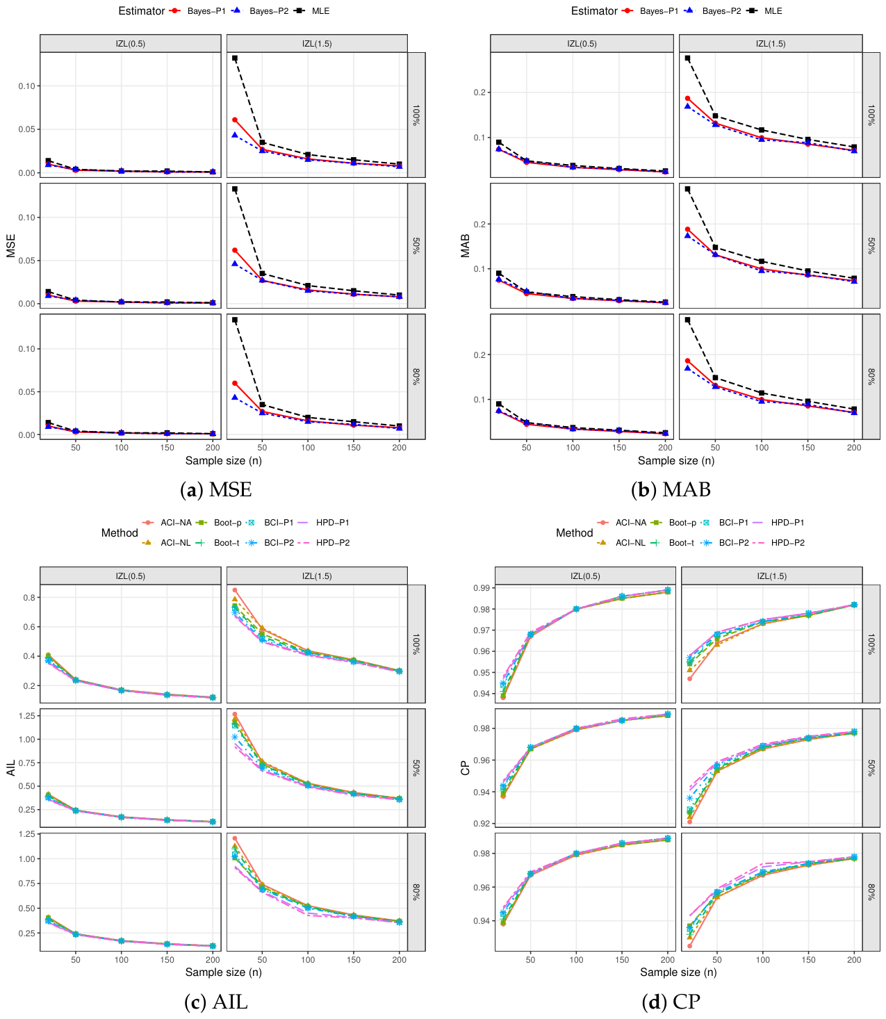
Figure 4 presents the simulation results for the IZL ( α ) model, summarizing the performance of competing estimators and interval construction methods across varying sample sizes and censoring proportions. The subplots in Figure 4a,b show that both MSE and MAB decrease steadily as the sample size increases, confirming the consistency of all estimators, with the Bayesian procedures (especially Bayes–P2) generally outperforming the MLE in small samples. The advantage of the Bayesian estimators is most pronounced under heavier censoring and smaller ( n ) , where the MLE exhibits noticeably higher variability. Figure 4c indicates that the AIL shrinks with increasing sample size, while BCIs, particularly HPD-based methods, tend to achieve shorter intervals compared to ACI-NA and ACI-NL methods without sacrificing stability. In Figure 4d, the CP approaches the nominal level as n grows, with Bayesian intervals showing slightly better adherence to the target level in small samples and under higher censoring. Overall, the results suggest that Bayesian approaches provide improved efficiency and more reliable interval estimation for the IZL ( α ) model, especially in challenging sampling scenarios. Additionally, all facts shown in Figure 4 support the same findings reported in Table 1 and Table 2.

7. Data Analysis

This section considers two real datasets gathered from engineering and health sciences, demonstrating the versatility and practical value of advanced inferential methods. The first dataset addresses environmental health by modeling the relationship between airborne contaminant exposure and urinary metabolite concentrations. In contrast, the second examines engineering reliability through the analysis of active repair times for airborne communication transceivers. Below, and before presenting these datasets in the Table 3, we offer the following brief discussion:
Data A:
Variations in airborne exposure levels to environmental contaminants can significantly influence the concentration of corresponding urinary metabolites, serving as critical biomarkers of internal dose. Understanding these fluctuations in airborne contaminant concentrations is reflected in urinary metabolite concentrations (UMCs), highlighting the dynamic relationship between external exposure and internal biological response; see Kumagai and Matsunaga [18]. We will reanalyze a dataset from Peter et al. [19] that includes 31 effects of variations in airborne exposure on UMC percentages.
Data B:
Airborne communication transceivers (ACTs) are critical components in aviation systems, and their active repair times constitute a key performance metric that directly influences operational readiness and mission continuity; see Tooley and Wyatt [20], for more details. These repair times show how well maintenance works, how complicated the transceiver hardware is, and how easily diagnostic tools can be accessed in both normal and urgent situations. This application examines 40 observations (measured in hours) of the active repair times for ACTs; see Jorgensen [21].
Table 3. Datasets from engineering and health sciences.
DataItems
UMC1.51.72.12.22.42.52.63.83.84.24.35.6
6.07.07.59.39.910.210.612.312.913.714.117.8
27.631.042.045.651.991.3131.8
ACT0.500.600.600.700.700.700.800.801.001.001.001.00
1.101.301.501.501.501.502.002.002.202.502.703.00
3.003.304.004.004.504.705.005.405.407.007.508.80
9.0010.2022.0024.50
Before proceeding further, the adequacy, flexibility, and practical effectiveness of the proposed IZL model are empirically assessed using the complete UMC and ACT datasets. Specifically, the fit performance of the IZL distribution is benchmarked against a comprehensive set of fifteen well-known inverted lifetime distributions available in the literature:
(1)
Inverted X-Lindley (IXL( α )) by Beghriche et al. [22];
(2)
Inverted Lindley (IL( α )) by Sharma et al. [6];
(3)
Inverted exponential (IE( α )) by Keller et al. [23];
(4)
Inverted Weibull (IW( θ , α )) by Ramos et al. [24];
(5)
Inverted gamma (IG( θ , α )) by Glen [25];
(6)
Inverted Chen (IC( θ , α )) by Srivastava and Srivastava [26];
(7)
Inverted Kumaraswamy (IK( θ , α )) by Abd AL-Fattah et al. [27];
(8)
Inverted Pham (IP( θ , α )) by Alqasem et al. [10].
(9)
Inverted exponentiated Pareto (IEP( θ , α )) by Abouammoh and Alshingiti [28];
(10)
Exponentiated inverted exponential (EIE( θ , α )) by Fatima and Ahmad [29];
(11)
Generalized inverted exponential (GIE( θ , α )) by Abouammoh and Alshingiti [28];
(12)
Inverted Nadarajah–Haghighi (INH( θ , α )) by Tahir et al. [30];
(13)
Inverted Lomax (ILo( θ , α )) by Kleiber and Kotz [31];
(14)
Alpha-power inverted exponential (APIE( θ , α )) by Ünal et al. [32];
(15)
Generalized inverted half-logistic (GIHL( θ , α )) by Potdar and Shirke [33].
The comparative adequacy of the IZL distribution relative to the competing lifetime models is examined using a collection of standard goodness-of-fit measures. Specifically, we consider (i) the negative log-likelihood ( L L ), (ii) the Akaike information criterion ( A I C ), (iii) the consistent AIC ( C A I C ), (iv) the Bayesian information criterion ( B I C ), (v) the Hannan–Quinn information criterion ( H Q I C ), and (vi) the Kolmogorov–Smirnov ( K S ) statistic together with its corresponding P-value. In Table 4, the aforementioned goodness-of-fit measures (i)–(vi) are computed using the MLEs of θ and α , along with their associated standard errors (Std.Ers). Inspection of Table 4 indicates that the proposed IZL distribution attains the lowest values across all considered metrics, while also yielding the highest p-value. These results collectively suggest that the IZL model provides a superior fit compared to the competing distributions, supporting its recommendation as the most appropriate model for the datasets under consideration.
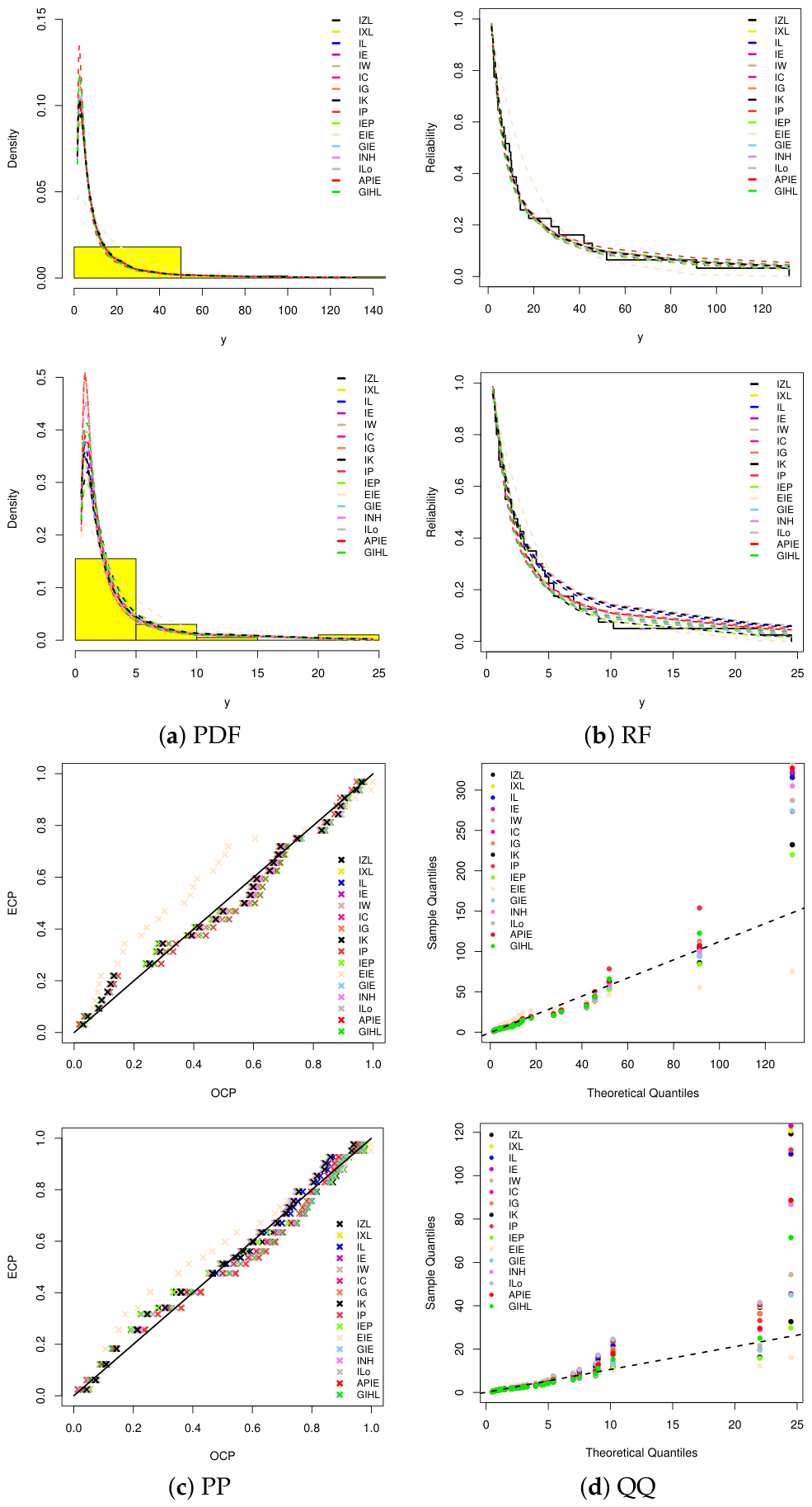
Figure 5 presents a comprehensive set of graphical goodness-of-fit diagnostics, the estimated PDF lines on UMC and ACT data histograms, and estimated/empirical lines of RF, P–P, and Q–Q functions to assess the adequacy of the proposed IZL distribution relative to several competing lifetime models. These diagnostics are applied to the UMC and ACT datasets to visually compare how well each model captures the empirical behavior of the observed data. Such graphical tools complement numerical fit criteria by revealing discrepancies in distributional shape, tail behavior, and overall agreement with empirical probabilities. Across both datasets, as shown in Figure 5, the IZL model exhibits closer alignment with the empirical distributions, as evidenced by tighter PDF overlays and P–P/Q–Q points lying nearer to the theoretical lines. This visual consistency supports the claim that the IZL distribution provides a superior or at least competitive fit, particularly in modeling skewness and tail characteristics of lifetime data.
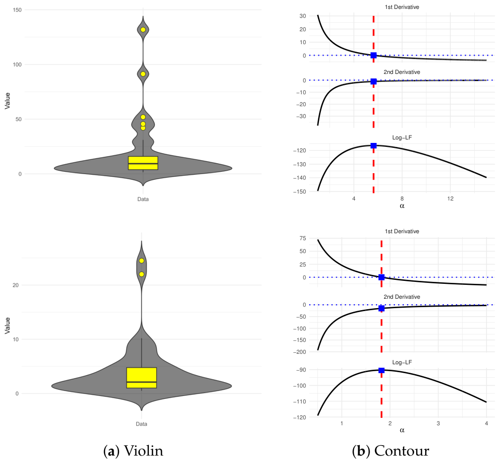
Additionally, Figure 6a,b illustrate complementary graphical tools for understanding the data structure and the behavior of the likelihood function in parameter estimation. The violin plots summarize the empirical distributions, highlighting skewness, dispersion, and the presence of extreme observations in each dataset.
It is worth noticing here that the proposed IZL distribution combines the ability to model a UBT hazard rate, positive skewness, and heavy-tailed behavior within a one-parameter framework. Hence, flexibility is reflected not only through numerical differences in the statistics fitted in Table 4 but also through the capacity to represent important lifetime mechanisms using a simple and interpretable model. It is also worth emphasizing that, in both the ACT and UMC datasets taken from communication engineering and environmental health, respectively, the IZL model attained the most competitive overall fit according to six standard criteria. Even when some competing models (e.g., IXL, IE, IL, IW, IG, INH, and GIE, among others) yield numerically close values, such closeness further supports the efficiency of the IZL model, since a one-parameter distribution remains competitive with more parameterized alternatives while preserving inferential simplicity. Accordingly, the empirical findings confirm that the IZL distribution is not only theoretically tractable but also a practically useful competitor for modeling lifetime data exhibiting skewness, heavy tails, and nonmonotone reliability behavior.
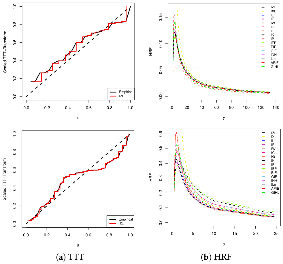
To further investigate the hazard-rate flexibility of the fitted models, Figure 7 displays graphical comparisons of the fitted HRF lines for both UMC and ACT datasets. Specifically, Figure 7a presents the empirical TTT transforms together with the fitted IZL TTT curves, while Figure 7b shows the estimated HRFs of the IZL model and all competing distributions. The empirical TTT plots (shown in Figure 7a) suggest non-constant failure mechanisms, supporting the need for flexible hazard-rate models. As shown in Figure 7b, the fitted HRF curve of the IZL model follows the empirical pattern closely compared to other competitors, indicating that the proposed model captures the principal reliability structure of both UMC and ACT datasets. Moreover, the hazard-rate comparisons reveal that, although some competing models yield numerically similar information criteria, several of them differ substantially in early-time behavior, peak intensity, or tail decline. By contrast, the IZL model provides a stable and interpretable hazard pattern with competitive overall agreement. To sum up, the graphical findings (shown in Figure 7a) are fully consistent with the formal goodness-of-fit results (listed in Table 4) and provide additional evidence that the proposed IZL distribution constitutes an effective and parsimonious model for positively skewed lifetime data with complex reliability behavior.
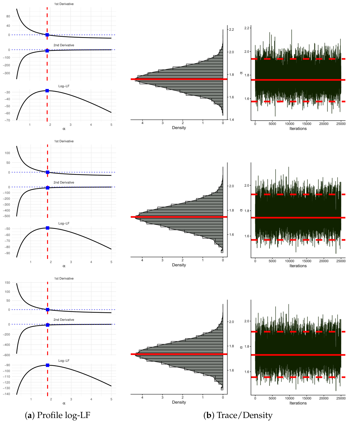
In parallel, the contour-style panels display the log-likelihood function and its first and second derivatives with respect to the parameter α , providing insight into the estimation process and curvature of the likelihood surface. For both datasets, Figure 6a indicates that the offered values of α are valid and unique; subsequently, these values are used as initial guesses for any subsequent computations involving α . For both datasets, Figure 6b indicates pronounced right-skewness and heavy-tailed behavior, justifying the use of flexible lifetime models rather than symmetric alternatives. Moreover, the zero-crossing of the first derivative together with the negative second derivative at the same point confirms the existence of a unique maximum of the log-likelihood, supporting the stability and reliability of the MLE for α .
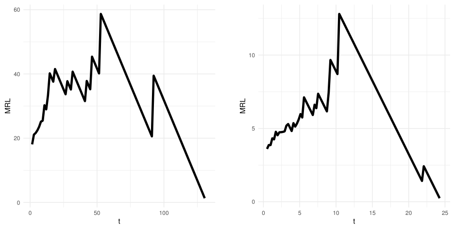
Empirical MRL analysis provides descriptive insight into the expected remaining lifetime of surviving units over the observed data range. Although the theoretical MRL in Theorem 4 is infinite due to the heavy-tailed structure of the IZL distribution, empirical MRL plots remain valuable practical tools for assessing residual-life behavior. Figure 8 shows that both the UMC and ACT datasets exhibit an overall UBT-shaped MRL pattern, characterized by an initial increase, followed by a peak and subsequent decline. This observed behavior is broadly consistent with a non-monotonic residual-life structure, indicating that the IZL model can effectively capture flexible and realistic lifetime dynamics in practical applications.
Using the complete UMC and ACT datasets, three T2CS samples were generated for each dataset under different values of j. For each sample S [ i ] ( i = 1 , 2 , 3 ), maximum likelihood and Bayesian estimates of the parameter α , along with their corresponding standard errors, were computed. Additionally, 95% interval estimates of α were obtained using asymptotic methods (ACI-NA and ACI-NL), bootstrap methods (Boot-p and Boot-t), and credible methods (BCI and HPD), with the corresponding interval widths recorded.
The selection of the hyperparameters ( ε 1 , ε 2 ) in the gamma prior can be guided by several practical considerations. In applications where prior information is available, the parameters ( ε 1 , ε 2 ) may be chosen to reflect expert knowledge about the scale of α . Alternatively, an empirical Bayes approach can be adopted by estimating ( ε 1 , ε 2 ) from the data, for example, via moment matching or marginal likelihood maximization. In the present study, since reliable prior information about α for the UMC and ACT datasets is not available, weakly informative gamma priors (e.g., with small values of ε 1 and ε 2 ) are employed to ensure numerical stability while avoiding undue influence on the posterior inference. Thus, a gamma prior with hyperparameters ε i = 0.0001 (for i = 1 , 2 ) was adopted to reflect near non-informative prior knowledge for the IZL ( α ) model. Posterior inference was performed using the M–H algorithm described in Algorithm 1, employing a burn-in period of 10,000 iterations and a total of 30,000 iterations.
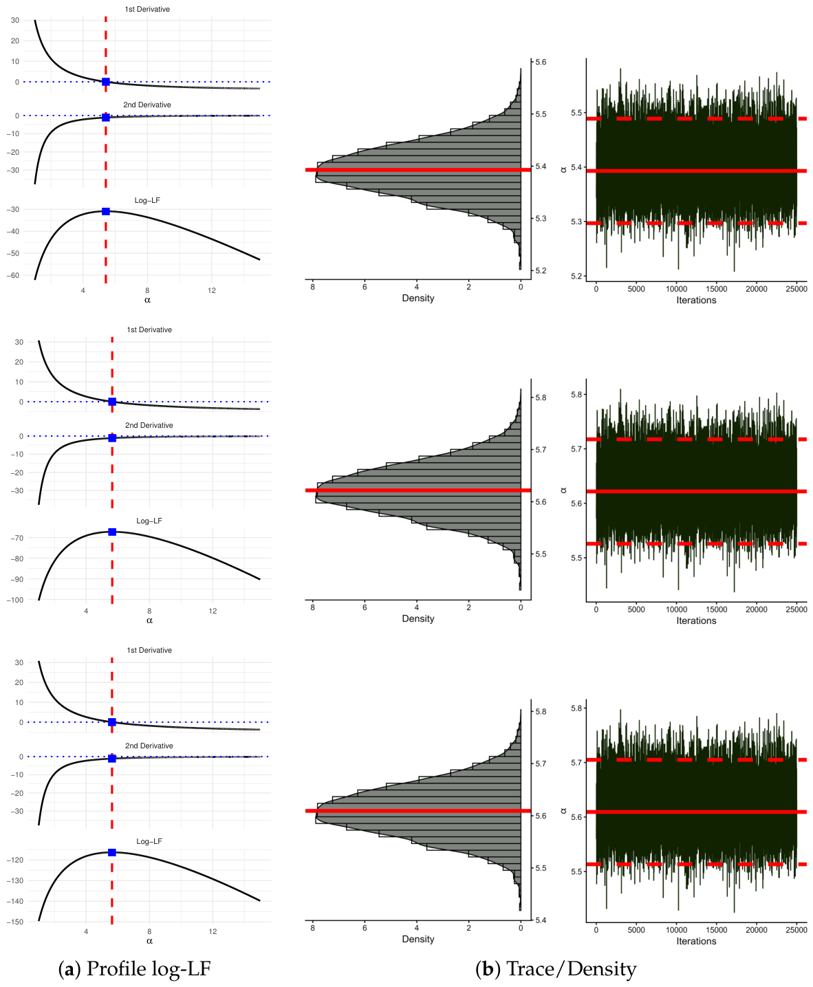
The existence and uniqueness of the MLE α ^ were examined via the profile log-likelihood function and its first and second derivatives, as illustrated in Figure 9 and Figure 10. The resulting plots exhibit clear, well-defined maxima, indicating that the MLEs obtained from all samples S [ i ] are unique for both datasets. The numerical estimates reported in Table 5 align with these graphical findings and were therefore used as initial values in the Bayesian analysis. A brief summary of useful statistics for the retained 25,000 MCMC samples of α is provided in Table 6. Furthermore, Figure 9 and Figure 10 present kernel density estimates and trace plots of the retained 25,000 MCMC samples of α , demonstrating good mixing and satisfactory convergence of the Markov chains. The approximate symmetry of the posterior samples further supports the adequacy of the selected burn-in period and confirms the reliability of the resulting Bayesian inference. These results demonstrate that both the frequentist and Bayesian methods provide reliable and consistent estimates of α across all censored samples created. In particular, the Bayesian approach, supported by MCMC diagnostics, exhibits robust convergence and efficient credible intervals, highlighting its suitability for inference under limited or censored data.
Overall, the results from the engineering and health sciences case studies demonstrate the versatility and practical value of the proposed IZL lifetime model for both complete and censored datasets. Specifically, the model effectively captures the dynamics of urinary metabolite concentrations in response to airborne contaminant exposure and accurately characterizes the active repair times of airborne communication transceivers, consistently outperforming fifteen widely used lifetime distributions and confirming its applicability to diverse real-world scenarios.

8. Conclusions and Future Perspectives

This study has introduced and systematically investigated a new one-parameter lifetime model, namely the IZL distribution, motivated by the need for parsimonious yet flexible alternatives to multi-parameter lifetime models commonly employed to capture non-monotone hazard behaviors. By leveraging an inversion mechanism, the proposed model successfully accommodates a UBT-shaped failure rate while maintaining analytical simplicity, interpretability, and computational feasibility. This balance between flexibility and parsimony represents a key contribution to contemporary distribution theory and reliability modeling. From a theoretical standpoint, the IZL distribution has been shown to possess rich structural properties. The density is strictly positive, unimodal, positively skewed, and heavy-tailed, while the hazard rate exhibits a unique unimodal shape with vanishing limits at both extremes. The derivation of an infinite-series expansion of the density provides a powerful analytical tool for studying tail behavior, moment existence, and approximation results. The explicit treatment of fractional moments, together with the formal justification for the non-existence of classical moments, highlights the importance of quantile-based and robustness-oriented summaries in heavy-tailed lifetime modeling.
Moreover, the availability of a closed-form quantile function through the Lambert W representation facilitates efficient simulation and supports both theoretical investigations and practical implementations. In terms of reliability analysis, the development of mean inactivity time and strong mean inactivity time functions enriches the interpretive capacity of the model, offering meaningful insights into system aging, downtime, and recovery dynamics. The explicit derivation of order statistics further broadens the applicability of the IZL distribution to extreme value analysis, stress–strength reliability, and system-level performance evaluation. Inferentially, the study provides a comprehensive framework for parameter estimation under Type-II censoring, encompassing likelihood-based and Bayesian methodologies. The existence and uniqueness of the maximum likelihood estimator ensure numerical stability, while Bayesian estimation via Markov chain Monte Carlo methods allows the incorporation of prior information and yields improved finite-sample performance. The comparative investigation of asymptotic, bootstrap, Bayesian credible, and HPD intervals demonstrates that Bayesian and HPD-based procedures are particularly effective in terms of estimation accuracy, interval length, and coverage probability, especially in censored and moderate-sample scenarios. The practical relevance of the proposed model has been convincingly demonstrated through applications to environmental health and communication engineering data. In both cases, the IZL distribution consistently outperforms a wide set of fifteen well-established inverted lifetime models across likelihood-based criteria, information measures, goodness-of-fit statistics, and graphical diagnostics. These empirical findings confirm that the proposed model is not only theoretically sound but also highly competitive in real-world applications involving skewness, heavy tails, and non-monotone failure dynamics.

8.1. Potential Research Directions

Several avenues for future research naturally arise from this work. First, the IZL framework may be extended to multi-parameter or regression-based versions by incorporating covariates, enabling its use in accelerated life testing, survival regression, and reliability modeling with explanatory variables. Second, the development of bivariate and multivariate extensions, possibly via copula constructions or shared frailty structures, would allow modeling of dependent lifetime data. Third, alternative censoring schemes, such as progressive, hybrid, or competing risk censoring, can be explored to further enhance the applicability of the model in complex experimental settings. Additionally, robust estimation techniques and goodness-of-fit tests specifically tailored to heavy-tailed inverted distributions merit further investigation.

8.2. Practical Recommendations

For practitioners in engineering and health sciences, the IZL distribution is recommended as a reliable and interpretable alternative when data exhibit early-life risk escalation, heavy tails, or unimodal hazard behavior. Bayesian inference with informative priors and HPD interval estimation is particularly advised in censored or small-to-moderate sample settings. Quantile-based summaries should be preferred over moment-based measures when describing central tendency and dispersion.
In summary, the proposed IZL distribution constitutes a meaningful contribution to modern lifetime modeling by unifying theoretical rigor, inferential robustness, and practical effectiveness within a parsimonious one-parameter framework. It opens several promising directions for future research while offering an immediately applicable tool for modeling complex reliability phenomena.
Ultimately, future research may investigate the applicability of the proposed IZL distribution beyond the two analyzed datasets, since its usefulness is not restricted to communication engineering and environmental health, but can be naturally extended to other domains such as finance, hydrology, insurance risk, biomedical survival studies, and industrial reliability data.

Author Contributions

Methodology, O.A.A. and A.E.; funding acquisition, O.A.A.; software, A.E.; investigation, O.A.A.; resources, A.E.; data curation, A.E.; supervision O.A.A.; writing—original draft, O.A.A. and A.E.; writing—review and editing O.A.A. and A.E. All authors have read and agreed to the published version of the manuscript.

Funding

The authors extend their appreciation to the Deanship of Scientific Research and Libraries in Princess Nourah bint Abdulrahman University for funding this research work through the Supporting Publication in Top-Impact Journals Initiative (SPTIF-2026).

Data Availability Statement

The authors confirm that the data supporting the findings of this study are available within the article.

Conflicts of Interest

The authors declare no conflicts of interest.

Appendix A. The CDF Validation

Proof. 
We demonstrate that the function F ( y ) defined in (3) constitutes a valid CDF and hence induces a proper probability measure on the interval ( 0 , ) . This is established by verifying the standard defining properties of a CDF: namely, that F ( y ) is (i) nondecreasing in y, (ii) right-continuous, and (iii) satisfies the boundary conditions lim y 0 + F ( y ) = 0 and lim y F ( y ) = 1 , as follows:
(i)
Monotonicity: We differentiate F ( y ) with respect to y. Let
g ( y ) = 1 + α 2 ( 1 + α ) y and h ( y ) = e α / y .
Then F ( y ) = g ( y ) h ( y ) . We compute
g ( y ) = α 2 ( 1 + α ) y 2 ,
and
h ( y ) = e α / y α y 2 .
Using the product rule,
F ( y ) = g ( y ) h ( y ) + g ( y ) h ( y ) .
Hence,
F ( y ) = e α / y α 2 ( 1 + α ) y 2 + 1 + α 2 ( 1 + α ) y α y 2 .
Factorizing α y 2 e α / y yields
F ( y ) = α y 2 e α / y 1 + α 2 ( 1 + α ) y 1 2 ( 1 + α ) .
After algebraic simplification, this becomes
F ( y ) = α y 2 1 + 1 2 ( 1 + α ) y e α / y .
Since y , α > 0 and the exponential term is strictly positive, we have F ( y ) > 0   for all y > 0 . Therefore, F ( y ) is strictly increasing and hence non-decreasing.
(ii)
Right-Continuity: The function F ( y ) in (3) is composed of rational functions and the exponential function. Both are continuous for y > 0 . Hence F ( y ) is continuous on ( 0 , ) , and therefore right-continuous on its support.
(iii)
Limiting Values: We now examine the boundary behavior.
  • As y 0 + : Since α / y ,
    e α / y 0 .
    Although the term α 2 ( 1 + α ) y diverges, the exponential term dominates the polynomial growth, and thus
    lim y 0 + F ( y ) = 0 .
  • As y :
    α y 0 , e α / y 1 , α 2 ( 1 + α ) y 0 .
    Therefore,
    lim y F ( y ) = ( 1 + 0 ) · 1 = 1 .
As a result, the CDF F ( y ) , given by (3), satisfies that
  • F ( y ) is non-decreasing on ( 0 , ) ;
  • F ( y ) is right-continuous;
  • lim y 0 + F ( y ) = 0 and lim y F ( y ) = 1 .

Appendix B. The Density and Failure Rate Shapes

This appendix investigates the structural behavior of the IZL distribution by examining the analytical shapes of its probability density and hazard rate functions. In particular, we establish the unimodality of the density and characterize the hazard rate behavior through rigorous asymptotic and monotonicity arguments.
  • (A): The Density Shape
Proof. 
We first examine the boundary behaviour of f ( y ) given by (4).
(i)
As y 0 + . Since α / y , it follows that e α / y 0 exponentially fast. The remaining polynomial term satisfies
α 2 ( 1 + α ) y 2 1 + 2 α + α y = O 1 y 3 , y 0 + .
Although Equation (A4) diverges polynomially, the exponential decay dominates any polynomial growth.
Hence,
lim y 0 + f ( y ) = 0 .
(ii)
As y . When y , we have α / y 0 and therefore e α / y 1 .
Moreover,
α 2 ( 1 + α ) y 2 1 + 2 α + α y α ( 1 + 2 α ) 2 ( 1 + α ) 1 y 2 .
Consequently,
lim y f ( y ) = 0 ,
with polynomial decay of order y 2 .
Thus, f ( y ) > 0 for all y > 0 , while f ( y ) 0 at both endpoints of ( 0 , ) . By continuity, the density attains at least one maximum on ( 0 , ) .
To investigate the uniqueness of the mode, consider the log-density
log f ( y ) = log α log 2 ( 1 + α ) 2 log y + log 1 + 2 α + α y α y .
Differentiating (A5) with respect to y yields
f ( y ) = d log f ( y ) d y = 2 y α y 2 1 + 2 α + α y + α y 2 .
From (A6), as y 0 + , the dominant term is α / y 2 , implying f ( y ) > 0 for sufficiently small y. As y , the dominant term is 2 / y , so that f ( y ) < 0 for sufficiently large y. By continuity of f ( y ) , there exists at least one y 0 > 0 such that f ( y 0 ) = 0 . Moreover, since f ( y ) changes sign from positive to negative, this stationary point is unique and corresponds to a global maximum. Therefore, the IZL density is unimodal for all α > 0 : it increases from zero, attains a unique mode, and then decreases monotonically to zero, exhibiting positive skewness. □
  • (B): The Hazard Rate Shape
Proof. 
We demonstrate the shape of the IZL hazard rate as follows:
(i)
t 0 + . Since α t , it follows that e α t 0 exponentially fast. Consequently,
f ( t ) = α 2 ( 1 + α ) t 2 1 + 2 α + α t e α t 0 ,
S ( t ) = 1 1 + α 2 ( 1 + α ) t e α t 1 .
Hence,
lim t 0 + h ( t ) = 0 .
(ii)
t . Using the first-order Taylor expansion
e α t = 1 α t + O 1 t 2 , t ,
we obtain
S ( t ) α ( 1 + 2 α ) 2 ( 1 + α ) 1 t , f ( t ) α 2 t 2 .
Therefore,
h ( t ) = f ( t ) S ( t ) 2 α ( 1 + α ) 1 + 2 α 1 t , t ,
which implies
lim t h ( t ) = 0 .
Thus, the hazard rate function is strictly positive for all t > 0 and vanishes at both boundaries of the support. Since h ( t ) is continuous on ( 0 , ) , it must attain at least one maximum in this interval. Moreover, for sufficiently small t, the numerator increases from zero while the denominator remains close to unity, implying that h ( t ) is increasing near the origin. For sufficiently large t, h ( t ) decreases proportionally to t 1 . Hence, the hazard rate function increases from zero, reaches a finite maximum, and then decreases monotonically to zero. Therefore, the IZL hazard rate function is unimodal and exhibits an upside-down bathtub (inverted-U) shape for all α > 0 . □

Appendix C. The Quantile Function

Proof. 
If Y I Z L ( α ) with the CDF (3), then its quantile function Q ( u ) = F 1 ( u ) , 0 < u < 1 , is obtained by solving F ( y ) = u for y. Set
u = 1 + α 2 ( 1 + α ) y e α / y , 0 < u < 1 .
Define v = α y y = α v , v > 0 . Then re-express (A7) as follows:
u = 1 + v 2 ( 1 + α ) e v .
Rearranging (A8) and multiplying both sides by 2 ( 1 + α ) , we get
2 ( 1 + α ) u e v = 2 ( 1 + α ) + v .
Let z = v + 2 ( 1 + α ) ; then Equation (A9) yields
2 ( 1 + α ) u e z 2 ( 1 + α ) = z .
Hence,
z e z = 2 ( 1 + α ) u e 2 ( 1 + α ) .
Multiplying both sides of (A11) by 1 ,
( z ) e z = 2 ( 1 + α ) u e 2 ( 1 + α ) .
Making use of the Lambert W function, defined by W ( x ) e W ( x ) = x , we obtain
z = W 2 ( 1 + α ) u e 2 ( 1 + α ) .
Therefore,
z = W 2 ( 1 + α ) u e 2 ( 1 + α ) ,
subsequently,
v = W 2 ( 1 + α ) u e 2 ( 1 + α ) 2 ( 1 + α ) .
Setting y = α / v , the IZL quantile function becomes
Q ( u ) = α W 2 ( 1 + α ) u e 2 ( 1 + α ) 2 ( 1 + α ) , 0 < u < 1 .

Appendix D. The rth Moments

Proof. 
The r-th non-central moment of Y is defined by
E ( Y r ) = 0 y r f ( y ; α ) d y .
Substituting the PDF (4) into (A17) yields
E ( Y r ) = α 2 ( 1 + α ) ( 1 + 2 α ) 0 y r 2 e α / y d y + α 0 y r 3 e α / y d y .
Consider the general integral
I k = 0 y k e α / y d y .
Using the transformation t = α / y , we have y = α t and d y = α t 2 d t , so Equation (A19) can be re-expressed as follows:
I k = α k + 1 0 t ( k + 2 ) e t d t = α k + 1 Γ ( k 1 ) ,
provided that k 1 > 0 , or equivalently k < 1 .
Applying the results in (A20) to the integral terms in (A18), we obtain
0 y r 2 e α / y d y = α r 1 Γ ( 1 r ) , r < 1 , 0 y r 3 e α / y d y = α r 2 Γ ( 2 r ) , r < 2 .
Substituting (A21) into (A18), we get
E ( Y r ) = α r 2 ( 1 + α ) ( 1 + 2 α ) Γ ( 1 r ) + Γ ( 2 r ) .
Note: Upon the term Γ ( 1 r ) , the r-th moment exists if and only if r < 1 , which completes the proof. □

Appendix E. The MRL Function

Proof. 
The MRL ( · ) of Y that follows the I Z L ( α ) model is given by
MRL ( t ) = 1 R t t R ( y ) d y = 1 R t ( t y f ( y ) d y t ) = 1 R t E ( Y ) I t , t > 0 .
Using (4), we now evaluate the integral term, I = 0 t y f y d y , in (A23) as follows:
I = 0 t y · α 2 ( 1 + α ) y 2 1 + 2 α + α y e α / y d y .
Thus,
I = α 2 ( 1 + α ) ( 1 + 2 α ) J 1 + α J 2 ,
where
J 1 = 0 t y 1 e α / y d y
and
J 2 = 0 t y 2 e α / y d y .
For J 1 , assume u = α y , y = α u , d y = α u 2 d u , and we obtain
y 1 d y = u α α u 2 d u = 1 u d u .
Updating the integral limits of J 1 in (A26) as
y 0 + u , y = t u = α t ,
yields
J 1 = α t e u u d u = α t e u u d u .
As a result, we get
J 1 = E 1 α t ,
where E 1 ( x ) = Γ ( 0 , x ) denotes the exponential integral.
Similarly, for J 2 in (A25), we set y 2 = u α 2 , d y = α u 2 d u , so that
y 2 d y = 1 α d u .
Thus,
J 2 = α t 1 α e u d u = 1 α α t e u d u = 1 α e α t .
Substituting (A31) and (A33) into (A25), we obtain
I = α 2 ( 1 + α ) ( 1 + 2 α ) E 1 α t + e α t .
Therefore,
MRL ( t ) = 1 R ( t ) E ( Y ) α 2 ( 1 + α ) ( 1 + 2 α ) E 1 α t + e α t t .
Since E ( Y ) = , the classical MRL diverges for all t > 0 , completing the proof. □

References

  1. Lindley, D.V. Fiducial distributions and Bayes’ theorem. J. R. Stat. Soc. Ser. (Methodol.) 1958, 20, 102–107. [Google Scholar] [CrossRef] [Scilit]
  2. Qayoom, D.; Rather, A.A.; Alsadat, N.; Hussam, E.; Gemeay, A.M. A new class of Lindley distribution: System reliability, simulation and applications. Heliyon 2024, 10, e38335. [Google Scholar] [CrossRef] [Scilit]
  3. Saaidia, N.; Belhamra, T.; Zeghdoudi, H. On ZLindley distribution: Statistical properties and applications. Stud. Eng. Exact Sci. 2024, 5, 3078–3097. [Google Scholar] [CrossRef] [Scilit]
  4. Alotaibi, R.; Elshahhat, A. Reliability Inference for ZLindley Models Under Improved Adaptive Progressive Censoring: Applications to Leukemia Trials and Flood Risks. Mathematics 2025, 13, 3499. [Google Scholar] [CrossRef] [Scilit]
  5. Mahnashi, A.M.; Zaagan, A.A. An improved version of ZLindley distribution with mathematical properties and applications. Alex. Eng. J. 2025, 129, 582–597. [Google Scholar] [CrossRef] [Scilit]
  6. Sharma, V.K.; Singh, S.K.; Singh, U.; Agiwal, V. The inverse Lindley distribution: A stress-strength reliability model with application to head and neck cancer data. J. Ind. Prod. Eng. 2015, 32, 162–173. [Google Scholar] [CrossRef] [Scilit]
  7. Nguyen, H.C.; Zecchina, R.; Berg, J. Inverse statistical problems: From the inverse Ising problem to data science. Adv. Phys. 2017, 66, 197–261. [Google Scholar] [CrossRef] [Scilit]
  8. Tomer, S.K.; Panwar, M.S. A review on Inverse Maxwell distribution with its statistical properties and applications. J. Stat. Theory Pract. 2020, 14, 33. [Google Scholar] [CrossRef] [Scilit]
  9. Choudhary, N.; Tyagi, A.; Singh, B. A flexible bathtub-shaped failure time model: Properties and associated inference. Statistica 2021, 81, 65–92. [Google Scholar]
  10. Alqasem, O.A.; Nassar, M.; Abd Elwahab, M.E.; Elshahhat, A. A new inverted Pham distribution for data modeling of mechanical components and diamond in South-West Africa. Phys. Scr. 2024, 99, 115268. [Google Scholar] [CrossRef] [Scilit]
  11. Singh, B.; Tyagi, S.; Singh, R.P.; Tyagi, A. Modified Topp-Leone Distribution: Properties, Classical and Bayesian Estimation with Application to COVID-19 and Reliability Data. Thail. Stat. 2025, 23, 72–96. [Google Scholar]
  12. Pavia, J.M.; Pavia, M.J.M. Package ‘GoFKernel’. Econom. Theory 2022, 10, 316–356. [Google Scholar]
  13. Yang, L.; Zhang, X.; Lu, Z.; Fu, Y.; Moens, D.; Beer, M. Reliability evaluation of a multi-state system with dependent components and imprecise parameters: A structural reliability treatment. Reliab. Eng. Syst. Saf. 2024, 250, 110240. [Google Scholar] [CrossRef] [Scilit]
  14. Henningsen, A.; Toomet, O. maxLik: A package for maximum likelihood estimation in R. Comput. Stat. 2011, 26, 443–458. [Google Scholar] [CrossRef] [Scilit]
  15. Dey, S.; Elshahhat, A.; Nassar, M. Analysis of progressive type-II censored gamma distribution. Comput. Stat. 2023, 38, 481–508. [Google Scholar] [CrossRef] [Scilit]
  16. Meeker, W.Q.; Escobar, L.A. Statistical Methods for Reliability Data; Wiley: New York, NY, USA, 1998. [Google Scholar]
  17. Plummer, M.; Best, N.; Cowles, K.; Vines, K. coda: Convergence diagnosis and output analysis for MCMC. R News 2006, 6, 7–11. [Google Scholar]
  18. Kumagai, S.; Matsunaga, I. Effect of variation of exposure to airborne chlorobenzene on internal exposure and concentrations of urinary metabolite. Occup. Environ. Med. 1995, 52, 65–70. [Google Scholar] [CrossRef] [Scilit]
  19. Peter, P.O.; Oluyede, B.; Bindele, H.F.; Ndwapi, N.; Mabikwa, O. The Gamma Odd Burr III-G Family of Distributions: Model, Properties and Applications. Rev. Colomb. Estad. 2021, 44, 331–368. [Google Scholar] [CrossRef] [Scilit]
  20. Tooley, M.; Wyatt, D. Aircraft Communications and Navigation Systems; Routledge: London, UK, 2024. [Google Scholar]
  21. Jorgensen, B. The hazard function. Lifetime models. In Statistical Properties of the Generalized Inverse Gaussian Distribution; Springer: New York, NY, USA, 1982; pp. 100–113. [Google Scholar]
  22. Beghriche, A.; Tashkandy, Y.A.; Bakr, M.E.; Zeghdoudi, H.; Gemeay, A.M.; Hossain, M.M.; Muse, A.H. The inverse XLindley distribution: Properties and application. IEEE Access 2023, 11, 47272–47281. [Google Scholar] [CrossRef] [Scilit]
  23. Keller, A.Z.; Kamath, A.R.R.; Perera, U.D. Reliability analysis of CNC machine tools. Reliab. Eng. 1982, 3, 449–473. [Google Scholar] [CrossRef] [Scilit]
  24. Ramos, P.L.; Louzada, F.; Ramos, E.; Dey, S. The Fréchet distribution: Estimation and application—An overview. J. Stat. Manag. Syst. 2020, 23, 549–578. [Google Scholar] [CrossRef] [Scilit]
  25. Glen, A.G. On the inverse gamma as a survival distribution. J. Qual. Technol. 2011, 43, 158–166. [Google Scholar] [CrossRef] [Scilit]
  26. Srivastava, P.K.; Srivastava, R.S. Two parameter inverse Chen distribution as survival model. Int. J. Stat. Mathemtika 2014, 11, 12–16. [Google Scholar]
  27. Abd; AL-Fattah, A.M.; El-Helbawy, A.A.; Al-Dayian, G.R. Inverted Kumaraswamy distribution: Properties and estimation. Pak. J. Stat. 2017, 33, 37–61. [Google Scholar]
  28. Abouammoh, A.M.; Alshingiti, A.M. Reliability estimation of generalized inverted exponential distribution. J. Stat. Comput. Simul. 2009, 79, 1301–1315. [Google Scholar] [CrossRef] [Scilit]
  29. Fatima, K.; Ahmad, S.P. The exponentiated inverted exponential distribution. J. Appl. Inf. Sci. 2017, 5, 35–41. [Google Scholar]
  30. Tahir, M.H.; Cordeiro, G.M.; Ali, S.; Dey, S.; Manzoor, A. The inverted Nadarajah–Haghighi distribution: Estimation methods and applications. J. Stat. Comput. Simul. 2018, 88, 2775–2798. [Google Scholar] [CrossRef] [Scilit]
  31. Kleiber, C.; Kotz, S. Statistical Size Distributions in Economics and Actuarial Sciences; John Wiley & Sons: Hoboken, NJ, USA, 2003. [Google Scholar]
  32. Ünal, C.; Cakmakyapan, S.; Özel, G. Alpha power inverted exponential distribution: Properties and application. Gazi Univ. J. Sci. 2018, 31, 954–965. [Google Scholar]
  33. Potdar, K.G.; Shirke, D.T. Inference for the parameters of generalized inverted family of distributions. Probstat Forum 2013, 6, 18–28. [Google Scholar]
Figure 1. Shapes for the PDF (left) and HRF (right) of the IZL model.
Mathematics 14 01566 g001
Figure 2. The log-LF and its score curves for the IZL parameter.
Mathematics 14 01566 g002
Figure 3. The likelihood, prior, and posterior shapes for the IZL parameter.
Mathematics 14 01566 g003
Figure 4. Maps for the simulation results of IZL ( α ) model.
Mathematics 14 01566 g004
Figure 5. Four fitting diagnostics for IZL and its competitors from UMC (top) and ACT (bottom) datasets.
Mathematics 14 01566 g005
Figure 6. The violin and contour diagrams for IZL model from UMC (top) and ACT (bottom) datasets.
Mathematics 14 01566 g006
Figure 7. The TTT and HRF lines from UMC (top) and ACT (bottom) datasets.
Mathematics 14 01566 g007
Figure 8. The MRL shapes from UMC (left) and ACT (right) datasets.
Mathematics 14 01566 g008
Figure 9. The existences and convergence diagrams of α from UMC data.
Mathematics 14 01566 g009
Figure 10. The existences and convergence diagrams of α from ACT data.
Mathematics 14 01566 g010
Table 4. Summary fit of the IZL and its competitors from UMC and ACT datasets.
ModelθαLLAICCAICBICHQICKS (p-Value)
Est.Std.ErEst.Std.Er
UMC Data
IZL--5.6340.950116.297234.595234.733236.029235.0620.0926 (0.9532)
IXL--5.3680.926116.304234.607234.745236.041235.0750.0928 (0.9514)
IL--5.9890.956116.452234.607234.747236.073235.0980.0929 (0.9516)
IE--5.2390.941116.305234.609234.747236.043235.0770.0932 (0.9504)
IW1.0260.1465.4121.372116.522236.578237.006239.446237.5130.0945 (0.9446)
IG1.0480.2355.4891.564116.516236.566236.995239.434237.5010.0949 (0.9429)
IC3.9091.0730.9260.149116.435236.405236.833239.273237.3390.1054 (0.8812)
IK1.1280.1877.6092.785116.505237.011237.439239.879237.9460.0966 (0.9345)
IP0.7590.1169.1522.959116.565237.130237.559239.998238.0650.1208 (0.7559)
IEP1.1790.2846.7461.513116.525237.050237.479239.918237.9850.0960 (0.9377)
EIE0.1190.0982.1481.645121.419246.838247.266249.706247.7730.2263 (0.0837)
GIE1.0480.2485.3991.253116.299236.570236.999239.438237.5050.0948 (0.9432)
INH1.1010.5934.5053.834116.521236.577237.006239.445237.5120.0961 (0.9370)
ILo21.2432.260.2560.405116.405236.810237.239239.678237.7450.0937 (0.9487)
APIE1.0631.2435.1611.755116.303236.607237.035239.475237.5420.0932 (0.9505)
GIHL0.8290.1840.1570.032116.715237.430237.858240.298238.3650.1182 (0.7790)
ACT Data
IZL--1.8230.25790.3186182.637182.743184.326183.2480.0896 (0.9049)
IXL--1.7500.23890.3864182.773182.878184.462183.3830.0905 (0.8988)
IL--2.0540.26190.4140182.658182.762184.396183.2520.0900 (0.9040)
IE--1.5470.24590.4865182.973183.078184.662183.5840.0936 (0.8749)
IW1.2080.1521.5690.24890.5252182.898183.222186.276184.1190.0953 (0.8610)
IG1.3530.2732.0940.51090.5264182.900183.225186.278184.1220.0959 (0.8552)
IC0.8420.1340.8680.11190.7478183.338183.662186.716184.5590.0982 (0.8356)
IK1.6620.2624.3331.23790.3735184.627184.951188.005185.8480.1072 (0.7470)
IP0.9040.1222.4330.22190.3275183.117183.441186.494184.3380.1020 (0.7997)
IEP1.9130.4423.2300.56690.6159185.232185.556188.609186.4530.1150 (0.6654)
EIE0.2790.1490.9950.45893.1216190.243190.568193.621191.4640.1936 (0.0999)
GIE1.3720.3001.8800.35890.4046182.977183.302186.355184.1990.0967 (0.8484)
INH2.7362.9910.3970.53390.5113182.870183.195186.248184.0920.0939 (0.8725)
ILo28.3661.690.0560.12590.7314185.463185.787188.840186.6840.0966 (0.8491)
APIE0.3480.3231.9650.44690.6389183.839184.163187.217185.0600.0899 (0.9042)
GIHL1.0470.2120.4600.07790.6063183.774184.099187.152184.9960.1009 (0.8105)
Table 5. Estimates of α from UMC and ACT datasets.
Sample ( n , j ) MLE95% ACI-NA95% Boot-p95% BCI
Bayes95% ACI-NL95% Boot-t95% HPD
Est.Std.ErLow.Upp.WidthLow.Upp.WidthLow.Upp.Width
UMC Data
S [ 1 ] (31, 10)5.41760.94833.55897.27623.71734.07828.37874.30055.29955.49150.1920
5.39290.04723.84427.63493.79063.50387.18963.68585.29705.48880.1919
S [ 2 ] (31, 20)5.64650.96223.76057.53243.77194.30358.09483.79135.52845.72040.1920
5.62180.07424.04317.88563.84243.96377.44303.47945.52575.71750.1918
S [ 3 ] (31, 31)5.63400.95603.76037.50763.74734.28328.03793.75485.51595.70790.1920
5.60930.08584.04007.85683.81683.96087.44243.48165.51335.70500.1918
ACT Data
S [ 1 ] (40, 15)1.85010.26811.32452.37561.05111.49172.38930.89761.57731.94260.3654
1.75910.13011.39262.45781.06531.43532.29390.85871.57541.93740.3620
S [ 2 ] (40, 25)1.83570.25941.32732.34411.01671.49562.41850.92301.56641.92750.3612
1.74510.12981.39172.42141.02981.39932.25710.85781.56961.92870.3591
S [ 3 ] (40, 40)1.82330.25671.32022.32641.00621.48792.36710.87921.55391.91490.3610
1.73290.12951.38362.40261.01901.40932.23820.82891.55721.91610.3589
Table 6. Summary for 25,000 Markovian iterations of α from UMC and ACT datasets.
Sample ( n , j ) MeanMode Q 1 Q 2 Q 3 Std.DSkew.
UMC Data
S [ 1 ] (31, 10)5.39295.26105.35945.39235.42640.04950.0529
S [ 2 ] (31, 20)5.62185.48995.58845.62125.65530.04950.0527
S [ 3 ] (31, 31)5.60935.47745.57595.60875.64280.04950.0527
ACT Data
S [ 1 ] (40, 15)1.75911.63161.69621.75971.82110.09290.0254
S [ 2 ] (40, 25)1.74511.51171.68251.74471.80740.09290.0300
S [ 3 ] (40, 40)1.73291.49931.67031.73251.79520.09280.0280
Disclaimer/Publisher’s Note: The statements, opinions and data contained in all publications are solely those of the individual author(s) and contributor(s) and not of MDPI and/or the editor(s). MDPI and/or the editor(s) disclaim responsibility for any injury to people or property resulting from any ideas, methods, instructions or products referred to in the content.