Light-Aware Modality Balancing Network for Multimodal Pedestrian Detection

Abstract

The visible light and infrared thermal multimodal images in autonomous driving provide a wealth of information for pedestrian detection, and its challenge lies in utilizing the complementary information across modalities to obtain an optimal joint representation. This study proposes a light-aware modality balancing network (LMB-Net) for pedestrian detection by fusing visible light and infrared thermal images. We designed an alignment complementary fusion module across modalities to exchange target information. Deformable convolutions are employed to automatically perform spatial deformation on features, thereby eliminating perception biases caused by misalignment. Furthermore, as the contribution of different modalities to pedestrian detection varies under different lighting conditions, we designed a light-aware module to utilize the distinct advantages of visible light and infrared thermal images. Extensive experiments on the KAIST and LLVIP datasets demonstrate that our method achieves the best detection performance compared to some other methods.

1. Introduction

Proactively identifying and avoiding pedestrians in scene perception is a crucial prerequisite for ensuring the safety of autonomous driving. The wavelength range of a pedestrian’s body temperature is clearly distinguishable under thermal imaging-based infrared cameras, and infrared cameras are also capable of detecting the temperatures of other objects in the environment. In conditions of glare or at night, infrared cameras can distinguish key targets in a scene more clearly than images captured by visible light cameras. Therefore, how to fuse visible light and infrared thermal information to achieve accurate and robust pedestrian detection is a challenge in autonomous driving scenarios [1].

In object detection tasks, most multimodal fusion models opt for feature-level fusion, and researchers have successively proposed methods for pedestrian detection using the fusion of visible light and infrared thermal data [2]. However, there remains room for improvement regarding how to effectively fuse multimodal information within the framework of deep convolutional networks. For these two types of multimodal data, including visible light and infrared thermal images, there exists a specific issue of illumination imbalance [3]. The illuminance imbalance refers to the difference in lighting conditions between day and night, a disparity that further leads to feature imbalance. For example, during the day, visible light images provide clearer textural features, whereas at night, infrared thermal images reveal more distinct pedestrian silhouettes. This implies that under different lighting conditions, the contributions of visible light images and infrared thermal images to the detection results are inconsistent. To address this problem, this study introduces a light-aware module capable of determining fusion weights based on lighting conditions, thereby mitigating the issue of lighting imbalance [4]. Furthermore, this study designed an alignment complementary fusion module by introducing deformable convolutions, aiming to enable the model to autonomously learn feature misalignment before fusing complementary information and perform corresponding spatial deformation adjustments. Experimental results demonstrate that the pedestrian detection model proposed in this study achieves a significant improvement in detection performance compared to other models.

The main contributions and innovations of this study include as follows:

(1)

We propose a light-aware modality balancing network for pedestrian detection by fusing visible light and infrared thermal images.

(2)

We design an alignment complementary fusion module across modalities to exchange target information by using deformable convolutions to predict the spatial transformations.

(3)

We design a light-aware module to more effectively utilize the distinct advantages of visible light and infrared thermal images.

2. Related Work

The supervised deep learning methods can be applied to the field of multispectral pedestrian detection. Researchers at Rutgers University [5] utilized convolutional neural networks to design fusion strategies at different stages, including low-level feature fusion, mid-level feature fusion, high-level feature fusion and result fusion, and this model is commonly referred to as Halfway Fusion. University of Bonn [6] has published papers on pedestrian detection using visible and infrared images, representing some of the earliest research on multispectral object detection based on deep learning. Pei et al. [7] compared the performance of additive fusion, maximum fusion, and concatenative fusion from the perspective of fusion methods. The Fusion RPN+BF model [8] introduces a region proposal generation network and a boosted decision classifier into this field. Most supervised methods merely apply deep learning techniques in a straightforward manner. However, with the advancement of computer vision and the deepening of research into multimodal data fusion, pedestrian detection based on visible light and infrared thermal images must not only address issues such as object occlusion and pedestrian crowding in visible-light pedestrian detection but also consider the effectiveness and robustness of multimodal fusion. To better integrate features from different modalities, CIAN [9] introduced a cross-modal interactive attention module to better utilize the complementarity of different modalities. Guan et al. [10] and Li et al. [11] pointed out that direct fusion of visible and infrared images suffers from an illumination imbalance, which hinders fusion performance. Consequently, they explored an illumination-aware mechanism (IAF R-CNN) that adjusts the weights of the day and night sub-networks by predicting illumination intensity. Zhang et al. [12] proposed a region-alignment network, AR-CNN, to process incompletely aligned multimodal data in an end-to-end manner. MSDS-RCNN [13] optimizes the model by combining the tasks of pedestrian detection and segmentation to enhance the performance of the detection model. Huang et al. [14] propose the cross-modal dual-flow feature interaction transformer (CDFIT), which decouples horizontal and vertical correlations to purify inter-modal attention, thereby aligning and fusing RGB and infrared features via dual-flow pathways. Zhou et al. [15] proposed a YOLO-based multispectral pedestrian detection method that enhances features through an adaptive multi-scale mask fusion module and utilizes a region-aware supervised feature alignment module to simultaneously achieve feature alignment and object-level displacement prediction. Wang et al. [16] proposed the Multi-scale Graph Spatial Alignment Network (MGSANet), which employs a graph attention network to model and mitigate the effects of cross-modal feature misalignment.

Some researchers have attempted to improve the performance of multispectral pedestrian detection through unsupervised modal transfer. Xu et al. [17] designed a cross-modal learning framework to model the relationship between visible and infrared images. Once the model is trained, it is transferred to the target domain, enabling robustness to changes in illumination even when only visible light images are available. Guan et al. [18] proposed a pedestrian detection framework for visible and infrared images, which updates the detector’s parameters in the target domain using pseudo-labels. Cao et al. [19] proposed an auto-framework that utilizes complementary information from multispectral data to annotate pedestrian instances in visible and infrared images. From the perspective of domain transfer, these studies have alleviated the issue of multimodal data scarcity to some extent and provided a solution for maintaining model robustness when data from a particular modality is missing. However, modal transfer generally yields lower accuracy than supervised learning methods, and the similarity between the source and target domains determines the upper limit of learnable knowledge. Shin et al. [20] proposed the semi-supervised multispectral pedestrian detector, SSMPD, which optimizes the quality of pseudo-labels through pedestrian appearance-aware weights, unified modal-aware synchronous learning, and similarity-based contrastive loss. Park et al. [21] proposed a fully unsupervised RGB-to-IR domain-adaptive object detection method. By utilizing generative models and large visual-language models to synthesize infrared images from RGB images via text prompts, it enables the training of domain-adaptive models without the need to collect real infrared data, significantly enhancing the robustness and efficiency of cross-spectral detection.

3. Methodology

3.1. Overall Network Architecture

The structure of the light-aware modality balancing network (LMB-Net) for pedestrian detection is shown in Figure 1. Based on the characteristics of visible and infrared thermal images, this network incorporates a light-aware module and an alignment complementary fusion module.

The LMB-Net utilizes ResNet50 as a backbone to ensure consistency between visible light and infrared thermal modal data, and the detail is listed in

Table 1. Convolution operations in the feature detection stage of the model.

Number of Stages	Procedure
Stage 1	Conv Block 64; Maximum Pooling
Stage 2	$\left[3*ConvBlock[64,64,256]\right]*3$
Stage 3	$\left[{\displaystyle \frac{3*ConvBlock[128,128,512]}{ACF}}\right]*4$
Stage 4	$\left[{\displaystyle \frac{3*ConvBlock[128,128,512]}{ACF}}\right]*6$
Stage 5	$\left[{\displaystyle \frac{3*ConvBlock[128,128,512]}{ACF}}\right]*3$
Stage 6	$\left[{\displaystyle \frac{3*ConvBlock[128,128,512]}{ACF}}\right]*1$

. The model’s feature extraction process comprises six stages, each consisting of convolutional modules that include convolutional layers, batch normalization layers and activation function layers. In stages three to five, the size of the feature maps is reduced using a stride of 2, while stage six does not involve any further size changes. From the third stage onwards, an alignment complementary fusion module (ACF) is connected at the end of each stage to achieve alignment of features from different modalities and the learning of complementary information. This design enables the fusion of features from the visible light and infrared thermal paths for use in the next stage of extraction. The output of the fusion module, together with the output from the previous stage, is fed into the next stage, while the residual connection is derived from the features prior to fusion. Ultimately, the outputs from the third to sixth stages comprise multi-scale feature maps, which are utilized for the pedestrian detection task.

3.2. Light-Aware Module (LAM)

A key advantage of fusing visible light with infrared thermal images is the ability to maintain detection capabilities even under poor lighting conditions. Generally, when lighting is sufficient, visible light images alone are adequate for recognizing and distinguishing pedestrians or other objects. However, in low-light conditions or when there is no external light source, infrared thermal images become the primary source for detecting pedestrians. It is evident that lighting conditions determine the modality dependency. However, pedestrian detection models cannot adaptively adjust the degree of reliance on different modalities based on lighting conditions. 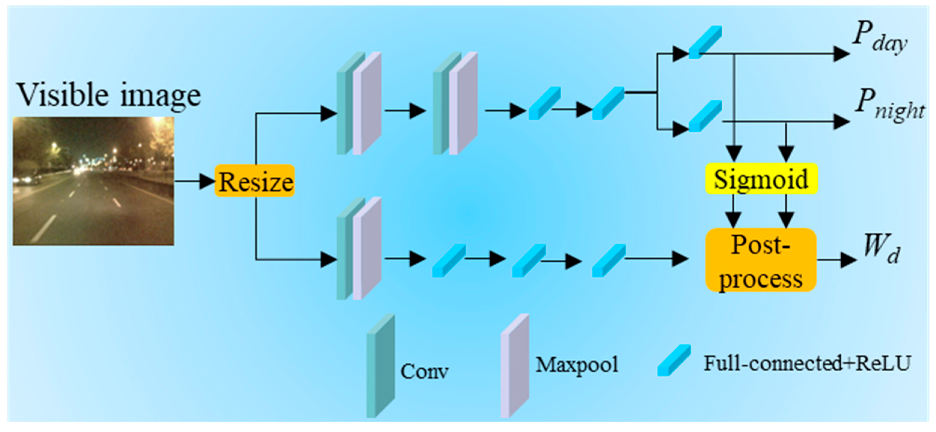Therefore, we introduce a light-aware module, the structure of which is shown in Figure 2. The key innovation of the proposed LMB-Net lies in constructing a light-aware modality balancing framework that adaptively adjusts the contributions of visible and thermal infrared modalities under varying illumination conditions, which is fundamentally different from the fixed or equal-weight fusion strategies widely adopted in previous works. This module captures differences in lighting conditions based on the visible light image, thereby outputting corresponding light-aware balance parameters. These parameters are utilized within the module to adjust the weights of features derived from visible light and infrared thermal modalities.

The preprocessing stage in Figure 2 is responsible for uniformly resizing all images input to the light-sensing module to a fixed dimension. Since assessing the overall brightness of an image does not depend on image details, this preprocessing step effectively reduces the number of network parameters and improves computational speed. The images are then fed into convolutional blocks, which consist of convolutional layers, batch normalization layers and activation layers; each convolutional block is followed by a max-pooling layer to further reduce the spatial dimensions of the feature maps. P_day and P_night represent the predicted values for daytime and night-time, respectively. As public datasets lack labels regarding light intensity, and since light intensity is a relatively subjective perception with a high degree of uncertainty in manual labeling, this module uses the time at which the image was captured as the standard for corresponding light intensity. Specifically, if the capture time is during the day, this indicates sufficient light, meaning that P_day should output a relatively higher score; conversely, at night, P_night should have a higher value. The output of this branch will be compared with the actual value, thereby updating the module’s parameters. Since P_day and P_night are intended to reflect actual light intensity, their output ranges tend to be close to 1 or 0, making them unsuitable for use directly in the model’s internal adjustment parameters. To address this, the light-aware module utilizes the output from the second branch to adjust the light balance parameters within the pedestrian detection model. The post-processing at the end of this branch adjusts the predicted scores based on a benchmark of 0.5, ensuring the results do not deviate excessively. The adjustment formula is shown below.

$$W_d={\displaystyle \frac{1}{2}}(P_{day}-P_{night})(\theta f+\beta )+{\displaystyle \frac{1}{2}}$$

(1)

where f refers to the features input into the post-processing module; θ and β are two learnable parameters within the post-processing module, initialized to 1 and 0, respectively. The final output, the daytime confidence score W_d, provides the light balance parameter for the model’s internal detection head.

3.3. Alignment Complementary Fusion Module (ACF)

To optimize the integration of information from the visible light and infrared thermal image modalities, we design an alignment complementary fusion module (ACF), which aims to efficiently fuse the features of two image types. Given the potential spatial misalignment between visible light and infrared thermal images, ACF specifically introduces a deformable convolution operation, aiming to adaptively learn spatial deformations without the need for additional supervision, thereby addressing potential spatial misalignment challenges. Furthermore, to ensure the quality of the fused features and maintain the network’s overall performance, we adopt the concept of a residual structure, ensuring that the fused features can be seamlessly integrated into the encoder branch. 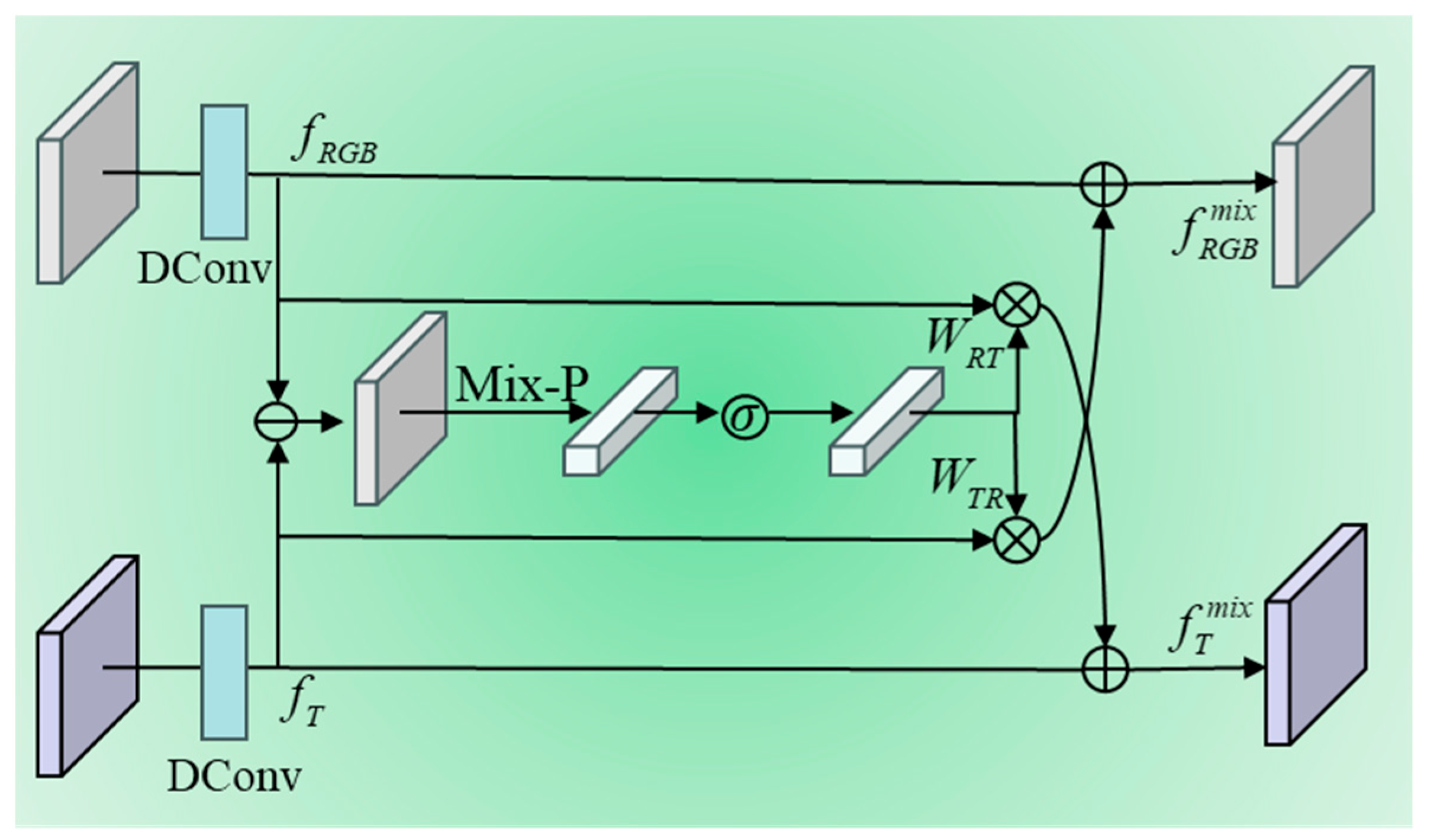Figure 3 provides a visual representation of the module’s architecture and working principle.

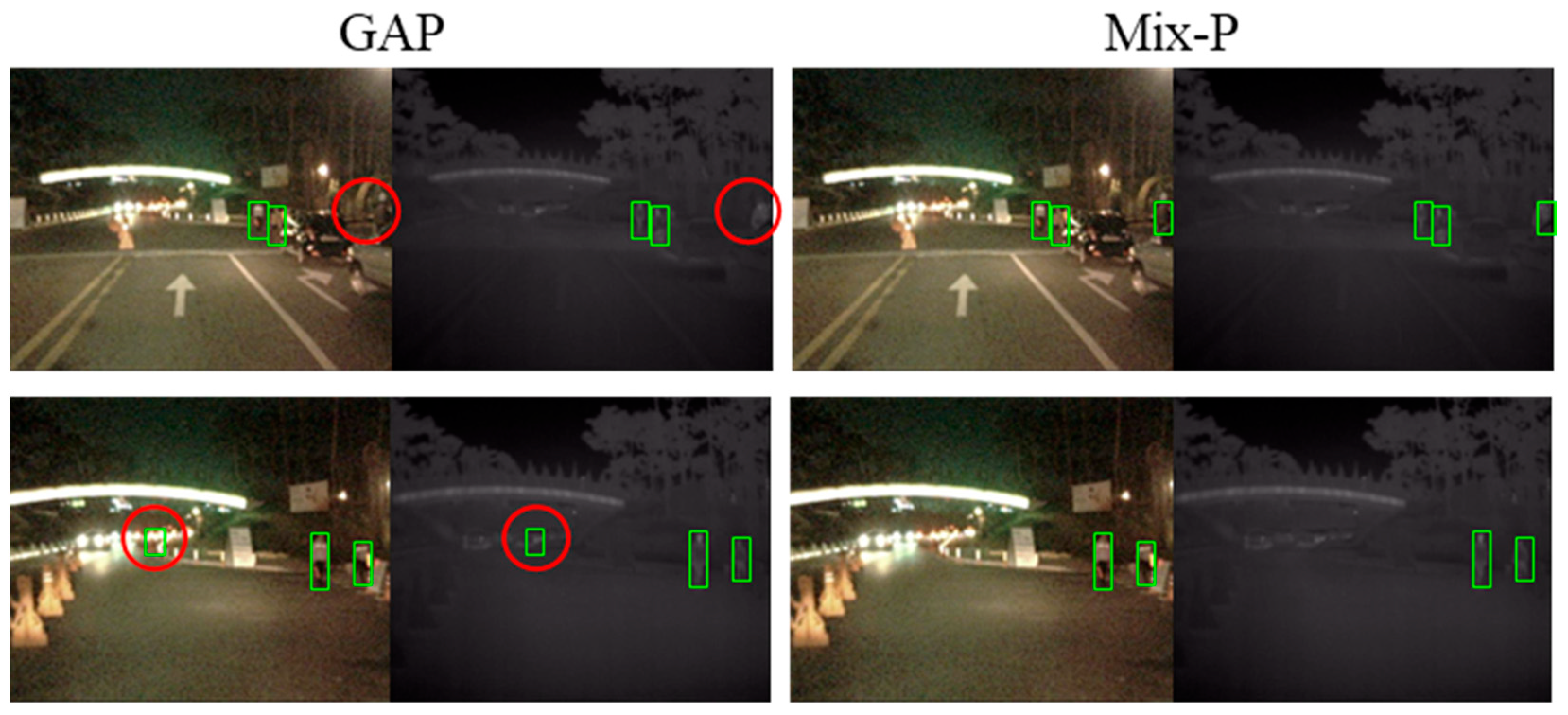
In Figure 3, we demonstrate how to fuse features from the two modal branches (visible light and infrared thermal) using the feature outputs from each stage of f_RGB and f_T by DConv operation. Taking the visible light features as an example, we first calculate the difference between f_RGB and f_T, aiming to emphasize the complementarity between the two modalities. We apply mixed pooling (Mix-P) [22] and the tanh activation function (θ) to this difference, thereby obtaining a complementary weight W_RT. For the infrared thermal branch, the corresponding complementary weight is denoted as W_TR. We then multiply W_RT by the original visible light feature f_RGB and add the result to the infrared thermal feature f_T to generate a fused feature $f_T^{mix}$. For the infrared thermal feature branch, we follow exactly the same procedure, except that the roles of the weights and features are swapped.

$$W_{RT}=\delta (\mathrm{Mix}(f_{RGB}-f_T))$$

(2)

$$W_{TR}=\delta (\mathrm{Mix}(f_T-f_{RGB}))$$

(3)

$$f_{RGB}^{mix}=f_{RGB}+W_{TR}·f_T$$

(4)

$$f_T^{mix}=f_T+W_{RT}·f_{RGB}$$

(5)

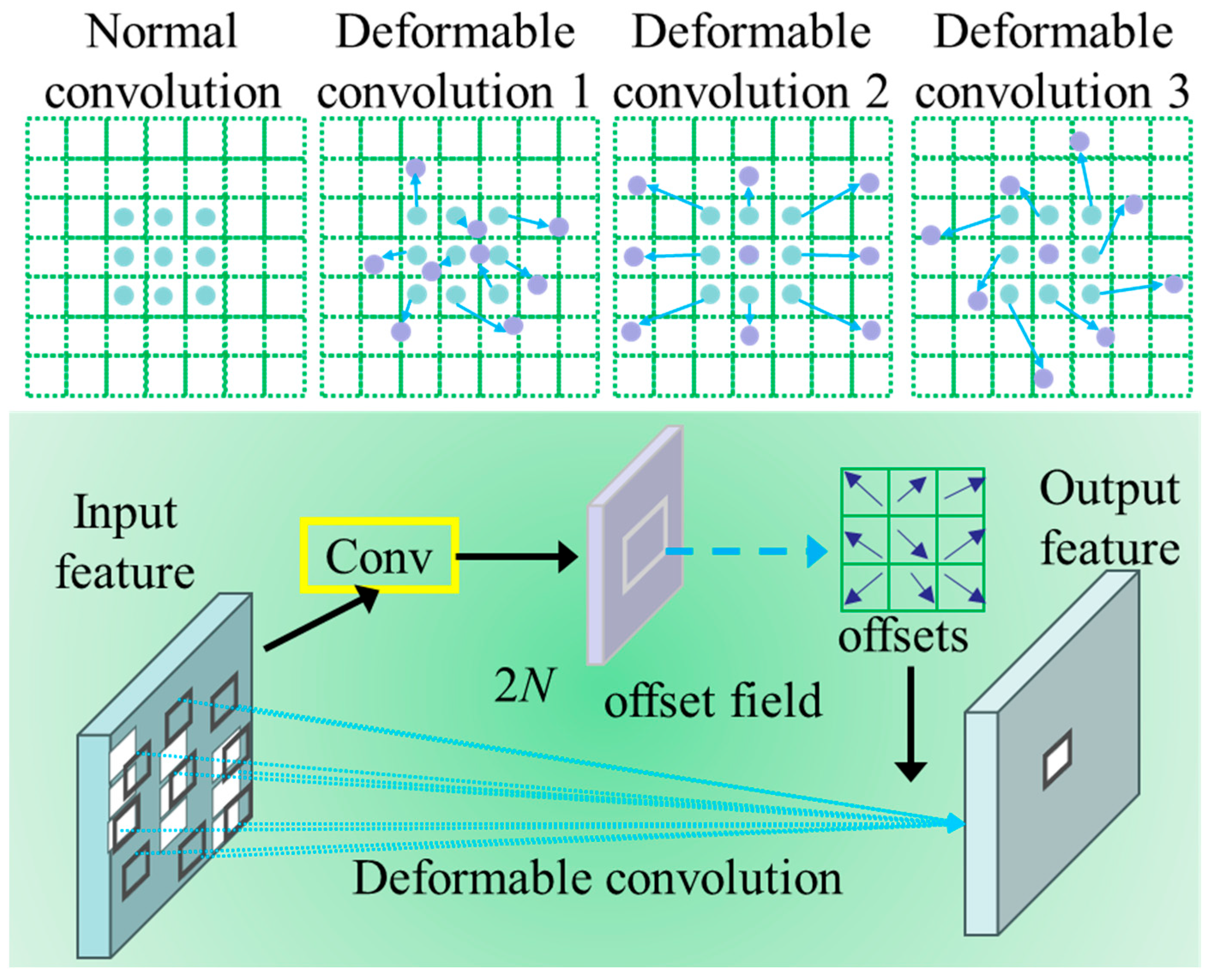
Figure 4 illustrates the key components of the deformable convolution operation, in which the size and shape of the kernel are variable. The figure clearly demonstrates how offsets are computed on the input feature map via a convolution layer. Specifically, this additional convolution layer generates an offset feature map with the same spatial dimensions as the input feature map, but with double the number of channels. The additional channels are used to predict offsets in the X and Y directions. These offsets are not fixed but are learned alongside the main task. In this way, deformable convolution can dynamically adjust its sampling positions to better accommodate the deformations and diversity of object shapes within an image. This plug-and-play nature enables deformable convolution to be easily integrated into various existing convolutional neural network architectures, thereby enhancing the network’s ability to process complex image features.

Deformable convolution is used to enhance the deformation modeling capabilities of convolutional neural networks. When discussing the role of convolution in image processing, traditional methods tend to sample at fixed grid points on the feature map. The consequence of this strategy is that, within each convolutional layer of a CNN, the internal activation units (neurons) possess receptive fields of identical size. They cover and influence regions of the same size within the input image. However, as the sizes and shapes of objects in the real world vary greatly, this rigidity inherent in traditional convolution limits its ability to effectively handle spatial deformations. To overcome this limitation, researchers have introduced the concept of deformable convolution, an improvement that incorporates the flexibility of two-dimensional spatial displacement into the sampling framework of traditional convolution. In this way, deformable convolution can better adapt to the diversity of objects within an image, enhancing the model’s ability to handle spatial deformations. Figure 4 illustrates the styles of traditional convolution kernels alongside various styles of deformable convolution. In convolutional neural networks, traditional convolution operations are constrained by their fixed sampling positions, resulting in a fixed receptive field for the convolution kernel. However, objects in real-world scenarios often vary in shape and size, requiring convolution operations to possess greater flexibility. Consequently, deformable convolution was developed, with its key feature being the introduction of dynamically adjustable displacements. These displacements are not predefined but are learned by the network during training. This means that deformable convolution kernels can adaptively adjust their shape and size according to the requirements of the actual task, thereby better capturing features within images. This adaptability enables deformable convolution, in theory, to handle deformations of arbitrary shapes, thereby enhancing the model’s ability to process complex image features.

3.4. Detection Head

The pedestrian detection model described in this study outputs the location and class information of pedestrians in an image via detection heads. Localization predictions are used to precisely localize the position of pedestrians within the image, while classification predictions are used to identify the class of the target, such as pedestrians or vehicles. This model design incorporates four independent detection heads, each responsible for generating detection boxes of specific scales and aspect ratios. Through this design, the model can effectively capture the location and category information of pedestrian targets at different scales, thereby improving the accuracy and robustness of detection.

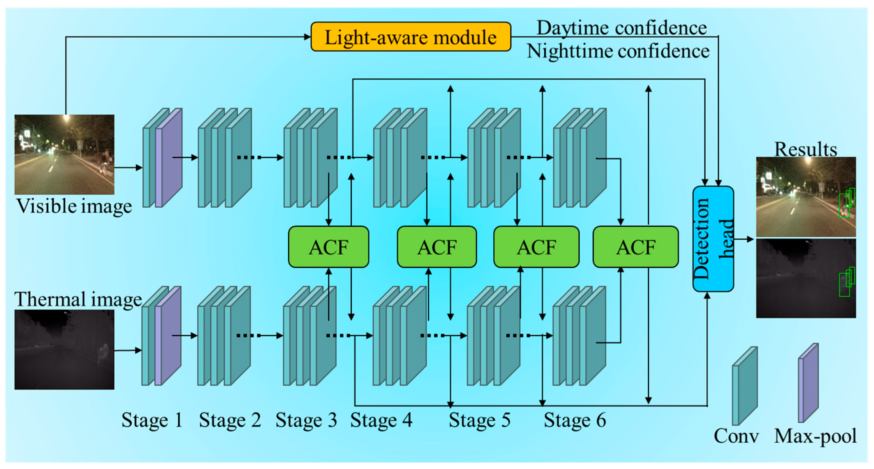
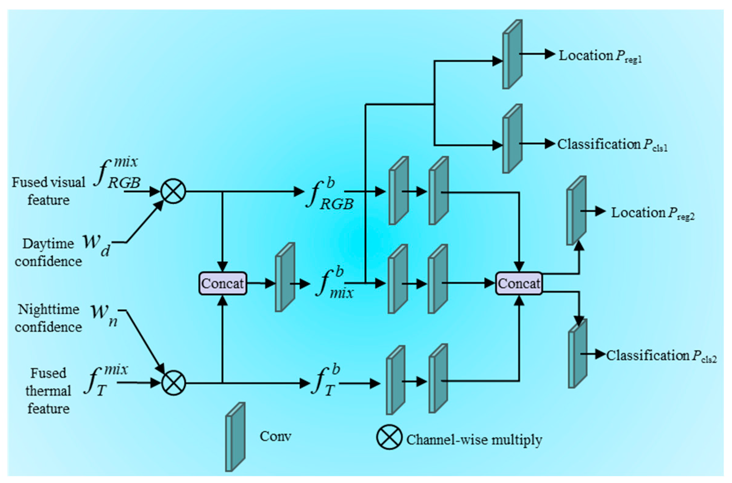
Each detection head focuses on multimodal feature detection at a specific scale, and the results from the four stages are merged to form the final detection output. This design allows the model to perform more aggressive weight reduction. Through the modal balance weights of the light-sensing module, it automatically adjusts the ratio of the two modal features and generates two sets of category-position outputs. In Figure 5, W_d represents the parameter obtained by the light-aware module from the visible light image. This can be understood as the degree of confidence we can place in the visible light image under the current lighting conditions. The confidence level of the infrared thermal image is calculated as W_n = 1 − W_d. These are weighted with the visible light and infrared thermal features respectively, yielding the weighted visible light feature $f_{RGB}^b$ and the weighted infrared thermal feature $f_T^b$. Concatenating these two features and feeding them into the convolutional block yields $f_{mix}^b$. We can see that a single detection head ultimately generates two sets of location-type results: one set is derived from the concatenated modal features, whilst the other is obtained by concatenating the unmerged modal information and then applying a convolutional operation.

3.5. Loss Function

In the final detection model, we define a total loss L_total, which consists of three key components: the light-aware loss L₁, the classification loss L_cls, and the localization loss L_reg. Together, these form the optimization objective during model training, and their mathematical expressions are as follows:

$$L_{total}=\lambda L_1+L_{cls}+L_{reg}$$

(6)

where hyperparameter λ is set to 1. Within the detection model’s loss function, the light-aware loss plays a crucial role and is expressed as

$$L_1=-Y_{day}\log (P_{day})-Y_{night}\log (P_{night})$$

(7)

which is based on the daytime prediction and night-time prediction P_night output by the light-aware module, as well as the corresponding ground-truth time-slot labels Y_day and Y_night. Specifically, when an image is actually captured during the day, the true label Y_day is 1, while Y_night is 0. Conversely, when an image is captured at night, Y_day is 0, while Y_night is 1. The calculation of the light-aware loss L₁ takes into account the differences between true labels and the predicted values, thereby ensuring that the model can accurately determine whether an image was captured during the day or at night.

In the loss function of the detection model, the classification loss L_cls and the localization loss L_reg each comprise two sets, reflecting the two distinct sets of outputs from the alignment detection module.

$$L_{cls}=L_{cls1}+L_{cls2}$$

(8)

$$L_{reg}=L_{reg1}+L_{reg2}$$

(9)

The first set of classification loss L_cls1 is calculated based on the first set of outputs from the detection head. The second set of classification loss L_cls2 is calculated based on the second set of outputs from the detection head. Similarly, for the localization loss, there are also two sets, including L_reg1 and L_reg2, which correspond to the localization losses of the two sets of detection results from the detection head, respectively. This design enables the model to evaluate the performance of the two sets of outputs more comprehensively and to optimize them simultaneously during training, thereby improving overall detection accuracy.

When discussing classification loss, as the calculation formulas for the two sets of classification loss (L_cls1 and L_cls2) are identical, we will present the definition and calculation process for classification loss collectively to simplify the explanation. Classification loss typically employs focal loss [23] as a metric, which is used to quantify the discrepancy between the model’s predicted classification results and the true labels.

$$L_{cls}=-\alpha {{\displaystyle {\sum }_{i\in pos}(1-P_{cls}^i)}}^{\gamma }\log (P_{cls}^i)-(1-\alpha ){\displaystyle {\sum }_{i\in neg}{P_{cls}^i}^{\gamma }}\log (1-P_{cls}^i)$$

(10)

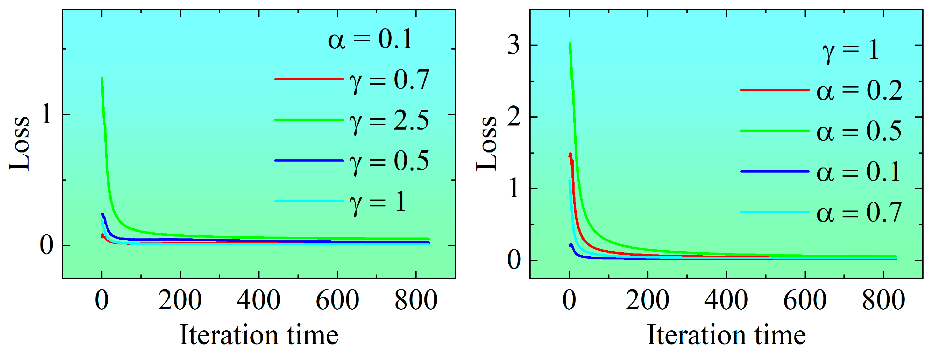
By minimizing this loss function, we can optimize the model parameters and improve the performance of the classification task. We define $P_{cls}^i$ as the predicted classification probability for the i-th detection box. To balance the contribution of positive and negative samples to the loss, we introduce a balancing factor α. To modulate the weight of hard-to-classify samples, we use a modulation coefficient γ. These two factors play a crucial role in the loss function, helping the model to better handle samples of different classes. The optimal values of α and γ in the unite loss function can be deduced as 0.1 and 1, respectively.

Localization loss is typically used to measure the discrepancy between the model’s predicted detection box position and the ground-truth detection box position.

$$L_{reg}={\displaystyle {\sum }_{i\in pos}SmoothL1(P_{reg}^i-Y_{reg}^i)}$$

(11)

We define $P_{reg}^i$ as the parametric coordinate offset of the model’s output for the i-th detection box. This represents the relative positional difference between the model’s predicted detection box and the predefined anchor box. Correspondingly, $Y_{reg}^i$ denotes the true parametric coordinate offset of the i-th detection box, i.e., the relative positional difference between the true detection box and the corresponding anchor box.

$$P_{reg}^i=\{P_x^i,P_y^i,P_w^i,P_h^i\}$$

(12)

$$Y_{reg}^i=\{Y_x^i,Y_y^i,Y_w^i,Y_h^i\}$$

(13)

For any given detection box in the detection model, the predicted parametric coordinate offsets are typically calculated based on the model output and the predefined anchor box. These parametric coordinate offsets are calculated as follows:

$$P_x=(x-x_a)/w_a$$

(14)

$$P_y=(y-y_a)/h_a$$

(15)

$$P_w=\log (w)/w_a$$

(16)

$$P_h=\log (h)/h_a$$

(17)

The parametric coordinate offsets typically involve the center x-coordinate, center y-coordinate, width, and height of the detection box. These coordinates and dimensions are usually compared with a predefined anchor box. Specifically, let $x,y,w,h$ denote the center x-coordinate, center y-coordinate, width, and height of the detection box, respectively, while the subscript a represents the anchor box, i.e., $x_a,y_a,w_a,h_a$ denote the center x-coordinate, center y-coordinate, width, and height of the anchor box, respectively.

In the calculation of the localization loss, to avoid the shortcomings of both L₁ and L₂ losses, we typically employ the $Smooth{L}_1$ loss.

$$Smooth{L}_1(x)=\left\{\begin{array}{cc}0.5x^2,\hfill & \left|x\right|<1\\ \left|x\right|-0.5,\hfill & other\end{array}\right.$$

(18)

It smoothly combines the characteristics of L₁ and L₂ losses, namely, it exhibits the behavior of L₂ loss (small gradient) where the error is close to zero, and the behavior of L₁ loss (constant gradient) where the error is large, thereby avoiding the vanishing gradient problem.

4. Dataset, Evaluation Metrics, and Implementation Details

The KAIST dataset [24] with an image size of 640 × 512 pixels contains 103,128 detection boxes and 1182 distinct pedestrians. The test set comprises 2252 image pairs, extracted from the raw video at a sampling rate of 20 frames per second, comprising 1455 daytime image pairs and 797 night-time image pairs. The dataset contains four categories, including clearly visible pedestrians (person class), individuals who cannot be distinguished (people class), cyclists riding two-wheeled vehicles (cyclist class), and unidentified objects that cannot be accurately distinguished (person? class). The classification criteria for pedestrian size are defined as follows: based on pixel height, pedestrians larger than 115 pixels are classified as large, those between 45 and 115 pixels as medium, and those between 1 and 44 pixels as small. The proportion of pedestrians in each size category, from largest to smallest, is 6%, 67%, and 27%, respectively.

LLVIP [25] is a high-resolution visible–thermal infrared paired pedestrian detection dataset, comprising a total of 16,836 pairs of registered infrared and visible light images, with 12,025 pairs used for training and 3463 pairs for testing. The majority of these were captured in very dark scenes, and all images are strictly aligned both temporally and spatially.

Figure 6 shows visible light and infrared thermal images from the KAIST and LLVIP datasets, respectively. As can be seen from the sample images, pedestrians are almost indistinguishable in the visible light images under poor lighting conditions or when there is little color contrast between the pedestrians and the background. In contrast, the corresponding infrared thermal images reveal the pedestrian’s outline with relative clarity.

We use the Log-average Miss Rate (LAMR) and mean average precision (mAP) as the evaluation metric on the KAIST dataset. We use mAP for evaluation on the LLVIP dataset.

Both training and testing in this paper were conducted on the Ubuntu 18.04 operating system, using an NVIDIA GeForce RTX 5070 Ti with 16 GB of VRAM. The model was built using the Python 3.6 and Keras 2.1 deep learning frameworks, with an initial learning rate set to 0.0001. The batch size and number of epochs were set to 8 and 50, respectively. The convolutional layers to be trained were initialized using the Xavier method. The feature extraction layer of the pedestrian detection model proposed in this study is first pre-trained on the ImageNet classification dataset. The weights of the pre-trained model serve as the initial weights. During training, these feature extraction layers with initial weights are frozen, while the remaining light-aware module, the alignment complementary fusion module, and the detection head continue to learn. As the pedestrian detection method proposed in this study is a single-stage detector, there is no candidate region proposal generation module. Therefore, predefined sizes and aspect ratios must be set for the detection boxes, i.e., prior boxes. The initial widths of the prior boxes in the third to sixth stages of this model are [25.84, 29.39], [33.81, 38.99], [44.47, 52.54], and [65.80, 131.40], respectively. Low-level features (shallow feature maps) are used to detect small-scale pedestrians, while high-level features (deep feature maps) are used to detect large-scale pedestrians at close range. The aspect ratio is set to 0.41 for all images. During training, data augmentation strategies involving horizontal random flipping and random color fluctuations will be applied to all training images.

5. Experimental Results and Analysis

5.1. Comparative Experimental Results

Table 2. LAMR metric of each method across different time intervals on KAIST test set.

Methods	All-Day	Daytime	Night
ACF	47.31	42.46	56.16
Halfway Fusion	25.56	24.87	26.58
Fusion RPN+BF	18.28	19.56	16.26
IAF R-CNN	15.72	14.54	18.25
CIAN	14.11	14.76	11.12
MSDS-RCNN	11.33	10.52	12.93
AR-CNN	9.33	9.93	8.37
Ours	8.01	8.34	7.89

presents the LAMR test results for different time periods on the KAIST dataset. It is clear that our model demonstrates significantly effective detection performance over other comparison methods across all time periods. This result demonstrates that our model exhibits exceptional perception capabilities in fusing visible light and infrared thermal modal information, further validating its stability and robustness under complex lighting conditions and across different time periods. As can be seen from the table, our model outperforms the other methods in detection performance across all time periods. The original benchmark method, ACF, had an LAMR as high as 47.32% under all-day conditions. Although it was considered a high-performing algorithm at the time, subsequent advancements in deep learning have enabled more comprehensive and robust feature learning, leading to progressively better detection performance. Halfway Fusion utilizes only the fusion of features from intermediate layers. Nevertheless, it can be observed that even this simple fusion resulted in an LAMR of 21.57% lower than that of ACF. However, as Halfway Fusion did not incorporate a dedicated fusion module specifically designed for visible light and infrared thermal images, there remains considerable room for improvement. Our model achieves LAMR of 8.01, 8.34, and 7.89 for all-day, daytime, and night-time scenarios, respectively, demonstrating that the proposed method makes effective use of the information provided by infrared thermal images at night.

Table 3. LAMR metric of various methods for pedestrians of different sizes on KAIST test set.

Method	Large	Medium-Sized	Small
ACF	28.73	53.66	88.19
Halfway Fusion	8.12	30.33	75.69
Fusion RPN+BF	0.05	30.88	88.87
IAF R-CNN	0.95	25.53	77.83
CIAN	3.90	19.03	55.81
MSDS-RCNN	1.28	16.18	63.72
AR-CNN	0.00	16.07	69.01
Ours	0.12	14.09	53.75

details the detection results for different pedestrian sizes on the KAIST test set for ACF, Halfway Fusion, Fusion RPN+BF, IAF R-CNN, CIAN, MSDS-RCNN, AR-CNN, and the method proposed in this study. Analysis of the data in the table reveals that all models exhibit low false negative rates when detecting large-sized pedestrians. However, upon comparing the different models, we find that while the proposed method does not entirely outperform the others in detecting large-sized pedestrians, its false negative rate is the lowest among all models when handling small and medium-sized pedestrians. This result fully demonstrates the advantages of our method in detecting small and medium-sized pedestrians, further validating its effectiveness in practical application scenarios.

The mAP performance comparison on the KAIST multispectral pedestrian detection benchmark (

Table 4. Comparison of mAP metric for each method on KAIST test set.

Methods	mAP0.5 (%)	mAP0.5:0.95 (%)
ACF	62.3	38.5
Halfway Fusion	72.4	41.2
Fusion RPN+BF	74.6	45.8
IAF R-CNN	78.9	50.2
CIAN	81.5	52.1
MSDS-RCNN	83.3	54.7
AR-CNN	82.7	53.6
AF-YOLOv8	74.6	34.2
Ours	83.6	55.4

) shows that the proposed method outperforms competing approaches, achieving the highest scores of 83.6% mAP@0.5 and 55.4% mAP@0.5:0.95. While traditional methods such as ACF and early fusion models lag significantly, advanced illumination-aware and attention-based detectors gradually improve performance, with MSDS-RCNN achieving the second-best results. The generic AF-YOLOv8 baseline exhibits limited performance, highlighting the need for specialized designs to fully exploit multispectral information in this challenging task. The consistent improvement over state-of-the-art competitors demonstrates the effectiveness of our approach in robust pedestrian detection across diverse illumination conditions.

Figure 7 shows the detection results for our model and compared methods, including IAF R-CNN, CIAN, and AR-CNN. Our method consistently aligns with ground truth across all samples, accurately localizing pedestrians in both visible and thermal modalities. In contrast, IAF R-CNN exhibits misalignment and redundant detections (marked by red circles) in the first and second samples, failing to fuse complementary modality information effectively. CIAN introduces false positives in the first sample, while AR-CNN suffers from localization drift in the second sample, indicating insufficient robustness to low-light and modality imbalance. These results demonstrate that our fusion strategy better exploits cross-modal cues, achieving advanced detection precision and alignment with ground truth, validating its effectiveness for nighttime pedestrian detection.

Table 5. Comparison of mAP metric for each method on LLVIP test set.

Methods	mAP0.5 (%)	mAP0.5:0.95 (%)
Faster R-CNN	93.1	56.8
CSSA	94.4	59.0
YOLOfuse	95.5	55.8
ICAFusion	95.8	59.0
MFYOLO	96.4	63.8
EI2Det	97.0	66.7
Ours	97.1	67.3

presents the quantitative comparison of mean average precision (mAP) metrics for multimodal pedestrian detection methods on the LLVIP test set. Two evaluation protocols are employed: mAP@0.5 (IoU threshold of 0.5) and mAP@0.5:0.95 (average over IoU thresholds from 0.5 to 0.95). Our proposed method achieves 97.1% mAP@0.5 and 67.3% mAP@0.5:0.95, outperforming all comparative approaches. Specifically, compared to the baseline Faster R-CNN, our method yields absolute gains of 4.0% and 10.5% in mAP@0.5 and mAP@0.5:0.95, respectively. Against state-of-the-art methods, including EI2Det (97.0% mAP@0.5, 66.7% mAP@0.5:0.95) and MFYOLO (96.4% mAP@0.5, 63.8% mAP@0.5:0.95), our method maintains consistent advantages, demonstrating robustness and detection precision across varying IoU thresholds. These results validate the effectiveness of our multimodal fusion strategy in leveraging complementary visible–thermal cues for low-light pedestrian detection.

Figure 8 illustrates the qualitative performance of multimodal pedestrian detection methods on nighttime visible–thermal road scenes, with ground-truth bounding boxes as the reference. Our proposed method achieves precise alignment with ground truth across all test samples, accurately localizing pedestrians in both modalities without redundant or missing detections. In contrast, Faster R-CNN exhibits obvious localization drift and false positives (marked by red circles), failing to effectively exploit complementary cross-modal cues. YOLOFuse maintains better alignment than Faster R-CNN but still shows minor localization bias in the first sample. ICAFusion introduces false negatives in the third sample, indicating insufficient robustness to low-light pedestrian instances. These results demonstrate that our multimodal fusion strategy better integrates visible and thermal information, leading to detection accuracy and alignment with ground truth, validating its effectiveness for complex nighttime pedestrian detection scenarios.

5.2. Ablation Study

To investigate in depth the specific contributions of the alignment complementary fusion module and the light-aware module to the performance of our proposed pedestrian detection model, we have carefully designed a series of ablation experiments, and the results are listed in

Table 6. LAMR for different modules at different time intervals.

ACF	LAM	All-Day	Daytime	Night
×	×	11.90	12.50	10.84
√	×	10.97	11.26	10.34
×	√	10.62	11.24	9.98
√	√	8.01	8.34	7.89

. Table 6 presents the LAMR of our multimodal pedestrian detection framework under different module combinations, evaluated across all-day, daytime, and nighttime scenarios on the KAIST dataset. The baseline without two modules yields the highest LAMR (11.90% all-day, 12.50% daytime, 10.84% nighttime). Activating ACF reduces LAMR to 10.97% (all-day), demonstrating its effectiveness in mitigating modality misalignment. Enabling LAM further lowers LAMR to 10.62% (all-day), validating its robustness to illumination variations. Integrating both modules achieves the minimum LAMR of 8.01% (all-day), 8.34% (daytime), 7.89% (nighttime), with absolute reductions of 3.89%, 4.16%, and 2.95% over the baseline. These results confirm the synergistic effect of ACF and LAM, which collectively enhance pedestrian detection recall across diverse lighting conditions.

Table 7. LAMR metric for different convolutions in ACF across different time periods.

Module	All Day	Daytime	Night
Normal convolution	10.96	10.32	11.32
Deformable convolution 1	9.37	9.64	9.12
Deformable convolution 2	9.03	9.27	8.94
Deformable convolution 3	8.01	8.34	7.89

reports the LAMR of our alignment complementary fusion (ACF) module with different convolution types, evaluated across all-day, daytime, and nighttime scenarios. Unlike normal convolution with fixed grid sampling, deformable convolution learns adaptive offset fields to adjust sampling positions, enabling better alignment of geometrically misaligned multimodal features. The baseline with normal convolution yields the highest LAMR of 10.96% (all-day), 10.32% (daytime), and 11.32% (nighttime). Deformable convolution·1 lowers LAMR to 9.37% (all-day), deformable convolution·2 to 9.03% (all-day), and deformable convolution·3 achieves the minimum LAMR of 8.01% (all-day), 8.34% (daytime), and 7.89% (nighttime). Notably, the LAMR reduction is more pronounced in nighttime (3.43% drop) than daytime (1.98% drop), indicating that deformable convolution better addresses low-light modality misalignment. These results validate that adaptive sampling via deformable convolution effectively enhances cross-modal feature alignment, reducing pedestrian miss rates and improving detection robustness across diverse lighting conditions.

Table 8. Ablation study for hyperparameter λ with LAMR metric.

λ	All Day	Daytime	Night
0.5	9.01	9.06	8.76
1	8.01	8.34	7.89
1.5	8.48	8.76	8.24
2	9.05	9.25	8.88
2.5	9.27	9.65	9.33

presents the ablation study on the weight λ of the light-aware loss, evaluated by the LAMR across all-day, daytime, and nighttime scenarios. The model achieves the optimal performance in all scenarios when λ = 1, with an all-day LAMR of 8.01%, a daytime LAMR of 8.34%, and a nighttime LAMR of 7.89%. When λ is too small (0.5) or too large (≥1.5), the LAMR increases significantly, leading to a continuous performance degradation. The analysis demonstrates that λ = 1 achieves the optimal trade-off for modality balancing. An excessively small λ weakens the illumination-aware constraint, failing to fully exploit the complementary advantages of visible and infrared modalities, while an overly large λ imposes excessive constraints on feature learning, undermining the generalization capability of the backbone network. These results validate the rationality of selecting λ = 1 as the weight of the light-aware loss in this work, providing experimental support for the robustness of the model in all illumination scenarios.

Figure 9 illustrates the focal loss function evolution with training iteration for different parameters α and γ. We compare the effects of different hyperparameters in focal loss on the convergence process of model training. In the left plot, with the learning rate α fixed at 0.1, the results show that when the modulation parameter γ is in the range of 0.5 to 1, the loss decreases rapidly and converges stably, whereas γ = 2.5 leads to a higher initial loss and a significantly slower convergence speed. In the right plot, with γ fixed at 1, the results indicate that α = 0.1 yields the fastest loss reduction and the lowest final convergence value, while α = 0.5 causes a sharp increase in initial loss and a noticeable lag in the convergence process. Overall, excessively large values of both γ and α weaken the effectiveness of gradient updates, resulting in degraded convergence performance, while moderate parameter settings enable the model to learn more efficiently during training and achieve a lower stable loss.

To verify the rationality of freezing the ImageNet-pretrained backbone, we perform an ablation study and report the LAMR results in

Table 9. Ablation study for pretrained backbone with LAMR metric.

Weight Pretrained Backbone	All Day	Daytime	Night
frozen	8.01	8.34	7.89
not frozen	9.34	9.64	8.37

. We compare two settings, including freezing the pretrained backbone and fine-tuning it under all-day, daytime, and night conditions, with other settings fixed. The results show that freezing the backbone effectively reduces the LAMR from 9.34 to 8.01 for all-day, 9.64 to 8.34 for daytime, and 8.37 to 7.89 for night, demonstrating clear performance improvements. The underlying mechanism can be explained by the trade-off between transferability and overfitting. The ImageNet-pretrained backbone encodes rich, general visual representations that are already highly compatible with our target scenes. Fine-tuning the backbone on our relatively limited dataset risks overfitting to scene-specific noise, such as illumination variations and cluttered backgrounds [26], thereby degrading generalization. In contrast, freezing the backbone preserves robust, low-level and mid-level features learned from large-scale data, stabilizing feature extraction and reducing miss rates. This strategy effectively avoids over-adaptation and maintains strong generalization across day and night conditions. Accordingly, freezing the pretrained backbone is experimentally verified to be the optimal choice for our model.

In the fully connected layers of ACF, a multi-pooling fusion method is employed rather than a single global average pooling. We utilize a fusion of global max pooling, global average pooling and global max-average pooling to improve the accuracy of image complementary alignment. As shown in Figure 10, a comparison between the improved Mix-P and the GAP reveals that the model using Mix-P exhibits a lower false negative rate when dealing with small-sized pedestrians.

6. Conclusions

This study proposes a light-aware modal balancing network to achieve multimodal image fusion for pedestrian detection using visible and infrared thermal images. The network employs residual modules based on an enhanced ResNet50 architecture, comprising two main components of a feature extraction head and a detection head, with the feature extraction head utilizing multi-level convolutional operations. We design an alignment complementary fusion module to address modality misalignment in multimodal pedestrian detection by leveraging deformable convolution to learn adaptive offset fields, enabling flexible sampling of complementary visible-thermal features. We design a light-aware module to enhance robustness to illumination variations by dynamically weighting modality-specific features according to ambient light conditions. Extensive experiments on the KAIST and LLVIP datasets show that our method achieves competitive performance and consistent improvements under the respective evaluation settings of each benchmark. Although our enhanced light-aware module significantly improves robustness to illumination variations, it still relies on a combination of capture time and simple global image statistics. In extreme cases, such as scenes with highly uneven lighting (e.g., strong backlighting and spotlight effects) or complex indoor environments, this approach may still produce inaccurate illumination estimates. In future work, we plan to develop a self-supervised illumination estimation network that can learn to predict illumination conditions from unlabeled images, thereby eliminating the need for any proxy variables.