


Abstract
This research entails comparative analysis and optimisation of machine learning models for regression and classification tasks on structured tabular datasets. The primary target audience for this analysis comprises researchers and practitioners working with structured tabular data. Common fields include biostatistics, insurance, and financial risk modelling, where computational efficiency and robust predictive performance are essential. Four machine learning techniques (i.e., linear/logistic regression, support vector machines (SVMs), Extreme Gradient Boosting (XGBoost), and Multi-Layered Perceptrons (MLPs)) were applied across 72 datasets sourced from OpenML and Kaggle. The datasets systematically varied by observation size, dimensionality, noise levels, linearity, and class balance. Based on extensive empirical analysis (72 datasets models configurations experiments), it is observed that, understanding the dataset characteristics is more critical than extensive hyperparameter tuning for optimal model performance. Also, linear models are robust across various settings, while non-linear models, like XGBoost and MLP, perform better in complex and noisy environments. In general, this study provides valuable insights for model selection and benchmarking in machine learning applications that involve structured tabular datasets.
Keywords:
machine learning; regression; classification; noise; balance; linearity; benchmark; hyperparameter tuning MSC:
62C05; 62H30
1. Introduction
People have developed a myriad of ways to benefit from machine learning techniques in different areas within a wide range of industries, from modelling insurance claims to predicting and diagnosing illnesses and even recommending adverts for items to purchase online, all based on key factors from collected data, see [1,2]. Not only is it beneficial for researchers to learn and understand the modelling used in everyday industries, it is also extremely important to gain an understanding and create a framework of why certain models work better under different data conditions. There are a few tried and tested techniques with regards to different industries, some working better than others depending on the data structure. Looking at most industries, data can be stored as unstructured or structured data. Structured data can be described as organised information that fits into a predefined formats, such as a table with rows and columns with numerical and categorical values, see [3]. Unstructured data, in contrast, does not have predefined formats and may include things such as free-text notes, images, and even audio recordings, see [4]. Note that it is possible to transform unstructured data into structured tabular data, but this requires extra pre-processing techniques.
Machine learning follows a general algorithm, which can be broken down into seven steps (see Figure 1). This process ensures that all the methods use a constant and robust process, even if the model parameters and mathematical makeup differ vastly. Machine learning can also be further broken down into multiple domains, two of which are our main focus in this paper (i.e., supervised and deep learning tasks), and unsupervised tasks.
Figure 1.
Machine Learning Steps, derived from [5].
Supervised learning is a subsection of machine learning, best described using a simple example: “Take a student learning from a teacher, where a teacher provides and teaches the student useful tools on how to solve problems. The student memorises these tools and then the student is able to collect and frame general rules on how to solve other similar problems and draw conclusions from it”. In supervised learning, the learning is performed using training data and its corresponding target response. Thus, for each observation of the predictor measurements where , there is an associated response measurement . The main goals for supervised learning can be defined as fitting a model that relates the response to the predictors in a way that means it is possible to accurately predict the response of future observations, while also allowing a better understanding of the relationship between the response and predictor variables (otherwise known as inference), see [2]. Popular types of supervised learning include models such as linear and logistic regression, random forest, and naive Bayes, just to name a few. All these models work on the same principle as stated above, relating a response variable () to predictor measurements (), though it must be noted that not all relationships are the same. With logistic and linear regression, for example, we can observe the following two equations and relationships for how each one’s response and predictor measurements relate differently, see [1]:
Clearly, we can see from our simple formulae above that indeed our models seem to have different ways of relating response and predictor variables. This is because of different types of transformations that we may come across, and as such different types of datasets require the strengths of different models. This is also true for deep learning. Supervised learning’s best forms of application are bio-informatics and speech recognition, as well as object recognition, to name a few.
Deep learning makes use of artificial neural networks with multiple layers to discover unique relationships between a set of inputs and outputs from a given dataset, see [1]. Deep learning methods can automatically discover hidden patterns within data, unlike traditional machine learning, which requires manual feature selection. These learned patterns are then used to make predictions, given sufficient compute power and large enough datasets. We can further expand the term of deep learning to the creation of deep neural networks, which in essence, means that we have neural networks with multiple layers. By adding more weights and biases, these neural networks can have improved capabilities and show improvements in predicting more complex functions, see [6].
The next few paragraphs provide an outline of how we derived the structured tabular dataset that we use for the analysis in this research work. This is done so that it is easy for the reader to visualise the attributes of the data used separately for regression and classification. More importantly, it should enable the reader to better understand the research objective and the corresponding research questions at the end of this section.
- Dimensionality: A grid (small, medium, large observations × small, medium, large features).
- Data quality: A grid (noise × imbalance or linearity).
- Model families: Linear, SVMs, XGBoost, and neural networks.
- Evaluation: Default vs. tuned configurations.
- Efficiency: Measured tuning time vs. performance gain.
Real datasets vary in size, dimensionality, and quality simultaneously. Studying these in isolation misses key interaction effects; however, the integrated design adopted in this research work provides a realistic understanding of how models behave across data scales and quality conditions.
Data was systematically obtained from the OpenML database using the API functionality. OpenML is an open source platform with access to free publicly available data. An API (Application Programming Interface) can be described as a set of protocols and tools that allow different software applications to communicate, such as connecting OpenML databases to a Python 3.9.18 downloading script. Databases were saved in the following format:
- obs_{size}x{feature_size}_Bal_{True/False}_Noisy_{True/False}_Type_{Task}_ID{openml_id}
The following is an example of how a dataset file name would be saved:
- obs_mediumxlarge_Bal_False_Noisy_True_Type_Regression_ID12345.csv
To systematically study the impact of data quality on model performance, each base dataset was transformed along up to three axes: noise level, class balance (for classification), and target linearity (for regression). Transformation was mostly done due to limited access to datasets that met all the requirements for what was needed in this study. The transformations, when needed, yielded the data-quality grids used in the factorial design.
For the noisy variants, additive Gaussian noise was introduced following the principle that perturbations should be scaled relative to the variability of each input feature [7]. Let denote a given numerical feature with empirical standard deviation . The standard deviation of the injected noise is defined as
For each observation, independent noise is added to the corresponding feature value. From [8], we can observe that the study used an array of 5–20% (factor of 0.05–0.20) in order to investigate noise level effects across different models. A factor of was selected to introduce a meaningful perturbation while preserving the overall structure of the underlying signal, and this can be adjusted to produce even noisier data in future studies.
For some classification datasets, class balance was manipulated to create both balanced and imbalanced variants of the main base dataset.
- Balanced datasets: The minority class was over-sampled using the Synthetic Minority Over-sampling Technique (SMOTE) [9], which generates synthetic minority examples in feature space to approximate balanced class proportions.
- Imbalanced datasets: Class imbalance was induced via random under-sampling, reducing one class to achieve a targeted skew in the class distribution (e.g., a majority/minority ratio greater than 1:1). Under sampling is a standard resampling technique for controlling class imbalance in experimental studies, see [10].
SMOTE generates synthetic samples by interpolating along line segments connecting minority class instances to their k-nearest neighbours. This mechanism has several geometric implications for class boundaries:
- Convex hull constraint: Synthetic points are generated strictly within the convex hull of existing minority samples, densifying sparse regions without extrapolating beyond the original feature space [9].
- Boundary smoothing: By filling gaps in the minority class distribution, SMOTE provides classifiers with stronger support for decision boundary placement, typically resulting in smoother, more generalisable boundaries.
- Overlap regions: In areas where classes naturally overlap, SMOTE may generate synthetic samples in ambiguous regions near the true decision boundary, potentially introducing label noise [10].
- Margin effects: For margin-based classifiers such as SVMs, synthetic points generated near class boundaries may reduce the separating margin between classes.
These geometric effects motivate the inclusion of both balanced and imbalanced conditions in the factorial design, enabling assessment of model robustness to SMOTE-induced boundary modifications.
In some dataset instances, the relationship between features and the target variable was controlled to produce both linear and non-linear variants, see [1,11]:
- Linear variants: Targets were generated from additive linear models of the formwith coefficients drawn from fixed distributions and denoting observational noise.
- Non-linear variants: Targets were generated using non-linear transformations of the features, for example, through polynomial terms, interaction effects, or smooth non-linear functions (e.g., sinusoidal components).
These transformations were applied to each of the nine dimensionality conditions, yielding the full design:
- Classification: Nine dimensionality conditions × (balanced vs. imbalanced) × (clean vs. noisy) datasets.
- Regression: Nine dimensionality conditions × (linear vs. non-linear) × (clean vs. noisy) datasets.
In total, this yielded 72 datasets spanning a broad range of data regimes in terms of sample size, feature dimensionality, noise level, class balance, and target linearity. All datasets were renamed to contain column TARGET_VARIABLE for consistency.
Standard feature processing was applied to the datasets and can be summarised as follows:
- Numerical features: Median imputation followed by standardisation (z-score scaling via StandardScaler).
- Categorical features: Mode imputation followed by one-hot encoding.
- Classification targets: Label encoding to 0-indexed integers.
Furthermore, no NaN post-imputation was applied (assert not np.isnan(X).any() before training), all features were sorted alphabetically before model fitting, and dataset sizes were capped for small, medium, and large observations in order to reduce total computational power and time needed for running models, capping them at {1000, 5000, 15,000} observations, respectively.
In this paper, we will be discussing popular machine learning modelling methods in both regression and classification problems, testing predictive performance under certain data conditions in both default and tuned states. In addition, we would like to investigate whether it would be realistic to create a framework/practical guide for model selection and whether or not there is some benefit into investing into deep learning for tabular data. This research work intends to answer these following questions:
- How does model performance scale with dataset size/dimensionality?
- Which models are robust to noise and imbalance/non-linearity?
- What is the performance gain vs. time cost of tuning?
- Is it possible to develop a practical guide for model selection?
- Is there some benefit in investing into deep learning for tabular data?
Four model families were evaluated symmetrically across both classification (36 datasets) and regression (36 datasets) tasks. Each family employs task-appropriate implementations: linear/logistic regression (Ordinary Least Squares (OLS) for regression, logistic loss for classification), SVM (Support Vector Regression (SVR) with epsilon-insensitive loss for regression, linear Support Vector Classification (SVC) with hinge loss for classification), XGBoost (squared error objective for regression, log-loss for classification), and MLP (Mean Squared Error (MSE) loss for regression, cross-entropy for classification). While the underlying algorithms differ by task, the architectural complexity and hyperparameter search spaces remain comparable within each family, enabling fair cross-task comparisons of model behavior under varying data conditions.
The remaining sections of the paper are structured as follows: Section 2 briefly discusses this study’s methodological approach (with a detailed discussion given in the Appendix A). Section 3 discusses the empirical analysis of the machine learning models applied to the datasets described above. Section 4 contains our concluding remarks, possible limitations and future research exploration.
2. Methodology
2.1. Linear Regression
Linear regression models the relationship between input features and a continuous target variable through a linear function:
and is optimised by minimising the sum of squared residuals (Ordinary Least Squares).
Default Configuration (scikit-learn OLS):
- Standard linear regression with no regularisation.
- Uses the library default fit_intercept = True.
Tuned Configuration (26 combinations × 5-fold CV = 130 fits).
Three regularised linear models were evaluated using cross-validation: Ridge (L2), LASSO (Least Absolute Shrinkage and Selection Operator) (L1), and elastic net (L1 + L2). The regularisation strength is controlled by , where larger values impose stronger penalisation on coefficient magnitudes. For elastic net, controls the mix between L1 and L2 penalties, with corresponding to pure LASSO and to pure ridge. The following hyperparameters were explored:
- Ridge regression (L2):
- LASSO regression (L1):
- Elastic net (L1 + L2):
- Model Selection Procedure:
- Evaluate all ridge variants (6 models).
- Evaluate all LASSO variants (5 models).
- Evaluate all elastic net variants (5 × 3 = 15 models).
- Select the best-performing model among all 26 candidates.
All models were implemented using CPU-only scikit-learn. Closed-form (OLS) and coordinate-descent solvers ensure computational efficiency even on large structured datasets.
2.2. Logistic Regression
Logistic regression models the probability of class membership through the following logistic function:
and is optimised by minimising the negative log-likelihood. A GPU-accelerated PyTorch 2.5.1+cu121 implementation using Stochastic Gradient Descent is used for both default and tuned configurations to ensure computational efficiency on large datasets.
Default Configuration:
- learning_rate .
- max_iter .
- batch_size .
Tuned Configuration (18 combinations × 5-fold CV = 90 fits):
Grid search was performed over the following hyperparameters:
- learning_rate .
- max_iter .
- batch_size .
2.3. XGBoost
2.3.1. Regression Study
Extreme Gradient Boosting (XGBoost) is a second-order tree-ensemble method that optimises a regularised objective function using gradients and Hessians. The algorithm is particularly well suited for structured tabular regression problems due to its ability to model nonlinear interactions and its built-in shrinkage and regularisation mechanisms. All regressors in this study were trained using GPU acceleration.
Default Configuration:
- n_estimators .
- max_depth .
- learning_rate .
- subsample .
- colsample_bytree .
Tuned Configuration (36 combinations, Random Search + 5-fold CV):
- n_estimators .
- max_depth .
- learning_rate .
- reg_alpha .
2.3.2. Classification Study
For classification tasks, XGBoost constructs an ensemble of decision trees optimised via additive boosting using a second-order approximation to the cross-entropy loss. GPU-accelerated training was employed for all experiments to ensure efficiency across high dimensions and large amounts of observational data.
Default Configuration:
- n_estimators .
- max_depth .
- learning_rate .
- subsample .
- colsample_bytree .
Tuned Configuration (12 combinations, Random Search + 5-fold CV):
- n_estimators .
- max_depth .
- learning_rate .
2.4. Support Vector Machines
2.4.1. Regression Study
SVR extends the principles of support vector machines to regression by fitting a function that deviates from the true targets by no more than an -insensitive margin. A linear kernel is used due to its computational efficiency and interpretability, see [1].
Default Configuration:
- .
- .
Tuned Configuration (12 combinations, Random Search + 5-fold CV = 60 fits):
- .
- .
2.4.2. Classification Study
SVC seeks a maximum-margin separating hyperplane and is well suited to high-dimensional structured data. A linear kernel was used for all datasets due to its computational efficiency and strong performance on linearly and near-linearly separable problems.
Default Configuration:
- .
- kernel = linear.
Tuned Configuration (6 combinations, Random Search + 5-fold CV = 30 fits):
- .
- class_weight .
2.5. Multi-Layered Perceptron (MLP)
The MLP was implemented using PyTorch with a feedforward architecture and the Adam optimiser [12]. The same configuration was used for both classification and regression tasks.
The default configuration uses hidden layers of [64, 32], a learning rate of 0.001, a dropout rate of 0.2, and a batch size of 32. Training was limited to 100 epochs with early stopping (patience of 10 epochs) to prevent over-fitting.
The tuned configuration consists of a total of 18 hyperparameter combinations, explored using a single 80/20 train/validation split. The tuning grid included hidden layers of [64], [128], and [64, 32], learning rates of 0.0001, 0.001, and 0.01, and dropout rates of 0.2 and 0.4.
Batch size (64) and optimiser (Adam) were held fixed during tuning. Training epochs were reduced to 50 during the hyperparameter search for computational efficiency; the best model was then refitted on the full training set with 100 epochs. This search space was designed to test depth, capacity, and regularisation effects while maintaining a feasible compute budget.
A hold-out approach was preferred over k-fold CV due to a number of factors such as training cost (900 vs. 4500 epochs), leading to a longer training time ( longer), and better GPU memory efficiency. This may have lead to worse performance, but it ensured shorter and more achievable training times/success rates.
2.6. Model Metrics: Regression
2.6.1. Evaluation Metrics
Primary model evaluation metrics for cross-dataset evaluations include the following:
- Normalised Root Mean Squared Error (NRMSE).
- Normalised Mean Absolute Error (NMAE).
- Normalised Mean Squared Error (NMSE).
- Training, prediction, and tuning time.
Note that normalisation is required for cross-data comparisons of within- and cross-model performance—see justification in next section.
2.6.2. Motivation for Normalisation in Regression Metrics
Regression metrics such as Root Mean Squared Error (RMSE), Mean Absolute Error (MAE), and MSE were used for cross-model evaluation. However, these metrics’ values are scale dependent, see [13], meaning these metrics all depend on the ranges and variances of the target variable of each independent dataset. This issue is a well documented problem, featuring in several machine learning studies and solved by normalisation. Article [14] defines the NRMSE as the RMSE divided by the standard deviation of the data (), and NMSE as the MSE divided by the variance of the data (). Looking at [15], NMAE indicates the mean deviation between the observed and predicted scores (MAE) divided by the standard deviations of the observed scores ().
Thus, for this study, the approach that was adopted in order to compare datasets was to correct for scale dependency by normalising the metrics using the population standard deviation of the target variable, denoted as . Note that classification metrics do not require any normalisation, see [16].
2.6.3. Cross-Dataset Overall Model Comparison by Rank
Due to different datasets varying in difficulty (noise, balance, dimensionality, etc.), even normalised performance metrics can over- or underestimate the actual model rank overall. In order to avoid this, we followed an evaluation protocol where we ranked a particular model on a scale—say, 1 for the best model, n for the last place, where n is the total number of models. We then take the average rank across all datasets (based on our normalised or standard metrics) in order to establish a mean rank across all dataset complexities.
2.7. Model Implementations: Classification
The primary model evaluation metrics for cross-dataset evaluations are F1-Macro, accuracy, Receiver Operating Characteristic–Area Under the Curve (ROC-AUC), and lastly training, prediction, and tuning time. Additionally, supplementary metrics for model evaluation that were tested for interest and comparison are precision, True Positive Rate (TPR), F1-score, precision-macro, recall-macro, Cohen’s Kappa, Mathews Correlation coefficient, and balanced accuracy; however, these metrics are only available in the raw results format. All primary metrics were selected based on common use in the literature, see [1,16].
2.8. Hyperparameter Optimisation Framework
2.8.1. Two-Level Tuning Strategy
- Default: Library defaults with no tuning.
- Tuned: Hyperparameter search using 5-fold CV (most models) or 80/20 holdout validation (MLP).
2.8.2. Tuning Budget per Model
Table 1 and Table 2 serve as short summaries on how tuning was performed across models for regression and classification, respectively.
Table 1.
Regression models—tuning budget.
Table 2.
Classification models—tuning budget.
2.9. Statistical Significance Testing
To determine whether observed differences in model performance are statistically meaningful rather than due to dataset-to-dataset variability, we apply recommended statistical tests for repeated measures across multiple datasets.
2.9.1. Friedman Test (Global Test)
The Friedman test [17] assesses whether multiple models differ significantly in their ranks across datasets. The Friedman test is the nonparametric analogue of repeated-measures ANOVA. It is appropriate in this context because model performance distributions are unknown, metrics are not normally distributed, and each model is evaluated on the same set of datasets. If the Friedman test is significant (), we reject the null hypothesis that all models perform equally.
2.9.2. Nemenyi Post Hoc Test (Pairwise Comparisons)
If the Friedman test indicates a significant global effect, the Nemenyi post hoc procedure is applied to compare models pairwise, see [18]. Two models i and j differ significantly if
where denotes the average rank of each model across datasets. Results are visualised using Critical Difference (CD) significance tables, displaying all the significant rank differences between the models.
2.9.3. Wilcoxon Signed-Rank Test (Optional Pairwise Test)
For targeted pairwise comparisons, such as evaluating default vs. tuned versions of the same model, the Wilcoxon signed-rank test was used. This test is nonparametric and well suited for paired measurements across the same datasets. It identifies whether one variant of a model consistently outperforms the counterpart without assuming normality.
2.10. Model Comparison Protocol
Within-model (default vs. tuned) comparison consisted of paired Wilcoxon signed-rank tests per model, ROI = score gain/tuning time. Between-model comparisons consisted of models being ranked by primary metrics of both classification and regression (F1-Macro and NRMSE). Statistical significance was assessed using Friedman tests with Nemenyi post hoc tests for pairwise comparisons.
GPU acceleration’s affect on training times reflects heterogeneous compute allocation: XGBoost and MLP leverage GPU acceleration (NVIDIA RTX 3090, CUDA 11.x), while linear/logistic regression and SVM execute on the CPU (AMD Ryzen 9 7900X, 12 cores/24 threads). Direct timing comparisons between GPU-accelerated and CPU-bound models should be interpreted with caution, as they measure different computational resources. The timing results are most meaningful for within-device comparisons (e.g., XGBoost vs. MLP on GPU) and for understanding the practical time cost of each approach given typical modern hardware configurations.
3. Final Results
A detailed account of the Python code that is used to generate these results can be found in the Supplementary Materials of this paper.
3.1. Regression
3.1.1. Overall Results
From Table 3, the extremely high descriptive statistics values observed for the MLP and SVM (as compared to those by linear regression and XGBoost) are consistent with the documented instability of gradient-based and margin-based regressors when exposed to high noise or heavily non-linear functions without strong regularisation, where SD denotes standard deviation.
Table 3.
Overall normalised regression performance (all datasets).
3.1.2. Model Ranking Across All Datasets
To compare models fairly across heterogeneous conditions, each model is ranked within each datasets using NRMSE (lower ranks = better performance). Average ranks across all datasets were then computed, and are reported in Table 4.
Table 4.
Average NRMSE-based ranks across all regression datasets (lower is better).
Table 4 shows that linear regression performing the best overall may be an early indication as to how some of the models failed catastrophically due to limited training budgets. This is clear from our overall results as well, seen in Table 3. The MLP and SVM having means NRMSE, NMAE and NMSE values shows that the metrics are out by around 3 standard deviations, which would influence the overall rankings negatively for certain datasets. However, these failures should not affect validity of the benchmark since the ranking and statistical tests rely on relative performance within each dataset, which should be evident when reviewing the full results.
3.1.3. Statistical Significance Testing
We applied the Friedman test to determine whether the differences in average ranks across models were statistically significant. The test returned
indicating highly significant differences between regression models. Since the global null hypothesis is rejected, the Nemenyi post hoc test is conducted. The CD at is . Table 5 summarises all statistically significant pairwise comparisons. A difference in average ranks greater than the CD indicates a significant difference in performance.
Table 5.
Significant Nemenyi post hoc comparisons for regression models.
Nearly all pairwise comparisons exceeded the CD, illustrating that the models differ substantially in performance. This result confirms the dominance of linear regression in this benchmark, as well as the instability of the SVM and MLP under challenging regression conditions with below-optimal hyperparameter tuning for these models.
3.2. Sensitivity Analysis: Excluding Extreme Model Failures
As shown in the primary analysis, a small subset of model–dataset combinations exhibited extremely large error values, especially for the SVM and MLP regressors on certain noisy non-linear datasets. These failures produced excessively large normalised error values (e.g., ), which unduly inflated the mean error metrics and distorted the distribution of model performance.
To verify that the overall conclusions were not driven by these pathological cases, we conducted a sensitivity analysis by restricting the evaluation to datasets where the NRMSE was less than 3. This threshold removed only the datasets where models diverged numerically, while preserving all normally-behaving instances. The resulting filtered subset represents a “well-behaved” regime, where all models—including the SVM and MLP—successfully converged and produced finite, meaningful predictions.
3.2.1. Updated Normalised Error Metrics
Table 6 reports the mean and standard deviation of the normalised metrics after exclusion of extreme RMSE outliers. Several key patterns emerge:
Table 6.
Overall normalised regression performance after filtering out failures (NRMSE < 3).
- Linear regression remains the top-performing model overall, both in default and tuned configurations, with mean .
- MLP performance improves substantially relative to the full dataset analysis, with mean – rather than the extreme values observed previously.
- XGBoost retains competitive performance, ranking closely behind linear regression.
- SVM improves considerably compared to the full dataset analysis, but still shows weaker performance than the other models, with .
3.2.2. Ranking Stability
Importantly, from Table 7, it is clear the relative ordering of models is consistent with the full analysis: linear regression remains the strongest model on average, followed by XGBoost, while SVM and MLP remain weaker, even when their extreme failure cases are removed.
Table 7.
Average NRMSE-based ranks across all regression datasets (NRMSE < 3).
3.2.3. Significance Testing
The Friedman test could not be applied meaningfully to the filtered subset, as some model–dataset combinations were removed by the RMSE threshold. This results in incomplete ranking matrices that violate the repeated-measures assumption required by the Friedman procedure [18]. Thus, statistical significance is not reported for the filtered sensitivity analysis.
3.2.4. Conclusion of Sensitivity Analysis
The RMSE sensitivity check confirms that the overall conclusions of the primary analysis are robust:
- Linear regression is consistently the strongest model across datasets, most likely due to it lacking a non-convex optimisation landscape and always converging to a closed-form or convex solution, making it inherently stable.
- XGBoost remains competitive but ranks below linear regression.
- MLP and SVM improve substantially when unstable cases are removed, but they do not surpass the top-performing models.
Therefore, the extreme error explosions observed for SVM and MLP on certain noisy non-linear datasets do not materially affect the primary findings. The ranking structure and relative ordering of models is stable under this sensitivity analysis.
3.2.5. Summary of Data Complexities
The rest of the results will be summarised by the mean model ranking per model complexity based on our primary metric, NRMSE, as well as overall mean ranking, with Table 8 summarising the results.
Table 8.
Best-performing regression models by data regime.
It is clear to see, from Table 8, that as a whole, the overall summary seems to accurately represent the expected results from our best performers. Some interesting key takeaways from these results are as follows:
- Linear regression with regularisation dominated the ranking metrics, placing highest on average across the board.
- For large and medium observations, XGBoost on a very basic tuning level competes really well with regression that has superior tuning. Regression dominates with small observations.
- Small dimensionality resulted in fairly good MLP performance, with linear regression dominating the medium and large ranges.
- Linear regression performed the best when the data was linear with respect to the target variable, whereas if the data was non-linear, XGBoost outperformed its competitors.
- Even though linear regression beat out the other models on noisy data, MLP performed very well under very light tuning and almost achieved the top rank and highest mean NRMSE score.
3.2.6. Tuning Effectiveness
Inspecting Table 9, we can see that across all regression models, XGBoost exhibited the strongest tuning efficiency. With a modest tuning time of approximately 106 s, tuning reduced the mean NRMSE by 0.0332, yielding the highest improvement per unit compute budget. Linear regression also benefited from tuning, although the effect was small (NRMSE ≈ 0.01) relative to its tuning time, resulting in a much lower ROI. Conversely, SVM showed essentially no improvement and MLP performed substantially worse after tuning, reflecting the well-documented instability of neural regressors under limited hyperparameter search budgets. These results demonstrate that hyperparameter tuning is most cost-effective for XGBoost in this experimental setting, while SVM and MLP yield little to no return for the same computational expenditure. The strong performance of linear regression in this study should not be generalised beyond the experimental context. Notably, the "tuning" process for linear regression represents a qualitative model selection, transitioning from unregularised OLS to the optimal regularisation strategy (ridge, LASSO, or elastic net), rather than incremental hyperparameter adjustment. This structural change yields substantial improvements that may not transfer to datasets with inherently non-linear relationships, where the model’s linear assumption becomes a fundamental limitation regardless of regularisation choice.
Table 9.
Tuning efficiency for regression models. NRMSE = Default − Tuned (positive values indicate improvement).
3.2.7. Wilcoxon Signed-Rank Test
To directly evaluate whether hyperparameter tuning improves individual model families, the Wilcoxon signed-rank test was applied to paired default–tuned NRMSE values across all regression datasets. The results shown in Table 10 demonstrate that tuning provides a statistically significant benefit for both linear regression () and XGBoost (), with the latter exhibiting a particularly strong effect. In contrast, tuning significantly worsened the performance of both the MLP regressor () and the SVM regressor (). These findings confirm the earlier observations from the ranking analyses: XGBoost is highly responsive to hyperparameter optimisation, while linear regression benefits only marginally. MLP and SVM, however, tend to degrade under the restricted tuning budget used in this study, reflecting their sensitivity to noisy or non-linear target structures and the tendency of limited searches to push them into unstable regions of hyperparameter space. It is also important to note that for MLP, under-performance may be budget-induced and not intrinsic to the model itself.
Table 10.
Wilcoxon signed-rank tests comparing default vs. tuned configurations for regression models using NRMSE. Positive outcome indicates that the tuned model performs significantly better.
3.3. Summary of Final Results: Classification
3.3.1. Overall Results
This section summarises the aggregate performance of all classification models across every dataset in the study. Three evaluation metrics are reported: macro-averaged F1 (F1-Macro), accuracy, and ROC–AUC. Because F1-Macro gives equal weight to minority and majority classes, it is used as the primary metric for statistical significance testing and ranking. Table 11 reports the mean and standard deviation of the three performance metrics across all classification datasets.
Table 11.
Overall classification performance across all datasets.
Overall, XGBoost (both default and tuned) achieves the strongest mean performance across all metrics. The MLP model is consistently competitive, while logistic regression and SVM lag behind in both F1-Macro and AUC.
3.3.2. Model Ranking Across All Datasets
Each model is ranked within every dataset using F1-Macro, where a higher F1-Macro score is better, resulting in a lower average rank that is closer to number 1. Table 12 reports the mean ranks.
Table 12.
Average F1-Macro ranks across all classification datasets (lower is better).
The ranking structure shows a clear grouping: XGBoost leads, followed closely by MLP. Logistic regression forms a middle tier, while SVM performs worst overall.
3.3.3. Statistical Significance Testing
The Friedman test is applied to determine whether observed differences in model ranks are statistically significant across repeated evaluation on the same datasets. The test returned
This indicates extremely strong evidence against the null hypothesis of equal performance.
Given the significant Friedman result, the Nemenyi post hoc test is applied. The CD at is . Table 13 summarises all statistically significant pairwise comparisons. A difference in average ranks greater than the CD indicates a significant difference in performance.
Table 13.
Significant Nemenyi post hoc differences (F1-Macro).
Nearly all significant contrasts are between the top-performing models (XGBoost and MLP) and the weaker baselines (logistic regression and SVM). There are no significant differences among the top three models: XGBoost (tuned), MLP (tuned), and XGBoost (default).
3.3.4. Summary
The overall classification analysis reveals the following:
- XGBoost (tuned) achieves the best performance across F1-Macro, accuracy, and AUC.
- MLP is highly competitive and statistically indistinguishable from XGBoost (default).
- Logistic regression performs moderately well but significantly below the top models.
- SVM is the weakest classifier across all datasets and differs significantly from all high-performing models.
- The SVM default and tuned versions performed similarly, possibly due to kernel simplicity/lack of options in tuning.
- There is no need to remove extreme values in this case, due to classification version of models not failing in the training/testing phases.
3.3.5. Summary of Data Complexities
The rest of the results will be summarised by the mean model ranking per model complexity based on our primary metric, F1-Macro, as well as overall mean ranking, with Table 14 summarising the results.
Table 14.
Best-performing classification models by data regime.
When inspecting Table 14, it is again clear that the overall summary seems to accurately represent the expected results from our best performers. Some interesting key takeaways from the results are as follows:
- Overall, the results and average metrics across all the models are extremely close, for both their default and tuned versions.
- XGBoost seems to be the highest ranked model overall across all the data complexities, but not by much, and in one case lost out to MLP tuned model, perhaps due to the structure of the data.
- XGBoost seems to have the best aggregate F1-Macro score as well, but again not by much.
3.3.6. Tuning Effectiveness
All models show an improvement, although minimal, when we apply tuning, as seen in Table 15. This may prompt further investigation as to whether the return on tuning is something significant and worthwhile for these different models.
Table 15.
Tuning efficiency for regression models. F1-Macro = Tuned − Default (positive values indicate improvement).
3.3.7. Wilcoxon Signed-Rank Results
Table 16 summarises the Wilcoxon statistic, associated p-value, and whether or not the tuned model performed better (yes/no for all models).
Table 16.
Wilcoxon signed-rank test results comparing tuned vs. default configurations for classification models (F1-Macro).
The Wilcoxon tests reveal several important patterns:
- None of the models exhibit statistically significant performance differences between default and tuned configurations at the level.
- SVM shows the strongest tuning effect (), suggesting that hyperparameters play a more influential role in margin-based models, although the improvement is not statistically significant.
- XGBoost and logistic regression show high stability between configurations, indicating that their default parameters already perform close to optimally across heterogeneous datasets.
- MLP shows slight improvements with tuning, but the effect is also not statistically significant.
The results demonstrate that, although tuning can provide marginal gains, the magnitude of these improvements is insufficient to reach statistical significance for any of the classification models. It is also important to note that for MLP, under-performance may be budget-induced and not intrinsic to the model itself. This aligns with the model-ranking analyses, where performance gaps between different model families were substantially larger than the differences between default and tuned configurations within the same family. Hyperparameter tuning therefore provides incremental rather than decisive improvements in typical classification scenarios.
3.4. Comparing Findings to Other Available Resources
AutoML benchmarks support a “start simple” heuristic, suggesting diminishing returns from complexity. Our finding of regularised linear models being competitive under constrained tuning supports this view. TabNet/FT-Transformer advance deep learning for tabular data, see [19,20]. Both methods strive to improve and provide architectural innovations for deep learning on tabular data. Though the MLP results are below par, our study does support the need for innovation in this space.
4. Concluding Remarks and Future Research
4.1. Concluding Remarks
Dataset size and dimensionality seemingly do have a significant impact on which model performs better, as different models perform the best in different categories in this study, hinting that data size and dimensions do matter. For this study, linear regression (tuned) seems to be the most robust for noisy data, whereas XGBoost performed the best for non-linear data. Performance gains via tuning do hint at extending hyperparameter tuning, as some models seem to suffer due to lack of extensive tuning, such as MLP. Developing a practical guide for model selection is a realistic approach, providing that all avenues and shortcomings that are discussed in the following sections are addressed and discussed.
- How does model performance scale with dataset size/dimensionality?
- Which models are robust to noise and imbalance/non-linearity?
- What is the performance gain vs. time cost of tuning?
- Is it possible to develop a practical guide for model selection?
- Is there some benefit in investing into deep learning for tabular data?
Although this study provides a comprehensive empirical evaluation of modern machine learning models across systematically varied dataset regimes, several avenues for future work remain open. These opportunities arise both from the limitations inherent to the present design and from natural extensions of the framework developed in this research.
- (1)
- Expansion of dataset diversity
This study utilised a controlled factorial structure spanning observation size, dimensionality, linearity, noise levels, and class balance. While this design ensured rigorous comparability, future work may incorporate the following:
- Domain-specific datasets (e.g., medical, financial, sports analytics).
- Real-world temporal or panel-based structures.
- High-dimensional feature spaces (e.g., genomic or text-based data).
- Heavily imbalanced or long-tailed label distributions.
- Larger-scale tabular data to test generalisation.
Such datasets would enable testing the generalisability of the findings to more complex applied contexts.
- (2)
- Alternative normalisation and evaluation strategies
This work utilised normalised regression metrics (NRMSE, NMAE, NMSE) to allow comparison across heterogeneous datasets. Additional efforts may investigate the following:
- Scale-free or distributional normalisation methods.
- Robust metrics (e.g., median absolute deviation forms).
- Probabilistic scoring rules for both regression and classification.
- Calibration-based evaluation, particularly relevant for clinical or risk-modelling contexts.
- (3)
- Statistical testing extensions
This study employed the Friedman and Nemenyi tests for multi-model comparisons, as well as Wilcoxon signed-rank tests for default vs. tuned configurations. Extensions may include the following:
- Hierarchical or mixed-model statistical frameworks.
- Effect-size estimation rather than purely significance-based methods.
- Post hoc Bayesian model comparison.
- Error decomposition and variance attribution across dataset factors.
These could provide deeper insight into how model performance varies as a function of dataset properties.
4.2. Future Research
- (1)
- Advanced deep learning methods
Some more modern and advanced applications of deep learning methods could be applied in order to possibly further differentiate between the effectiveness of deep learning and the more traditional methods used in classification and regression, also allowing us to differentiate between different deep learning architectures, such as the following:
- Attention-based models.
- Residual/MLP-enhanced architectures.
- Specialised tabular neural architectures.
- Hybrid neural–tree models.
Exploring more advanced deep learning methods may be beneficial, as deep learning is already being used more extensively today due to hardware and software performance acceleration. This is also true for tabular data: as deep learning architecture advances, the results seem to improve, see [19,20].
- (2)
- Advanced Hyperparameter Optimisation
The results indicate that tuning yields relatively small improvements compared to differences across model families. Future work may therefore consider the following:
- Bayesian optimisation with early stopping.
- Adaptive multi-fidelity search.
- Model-based optimisation under strict time or computation budgets.
- Automated machine learning (AutoML) approaches incorporating meta-learning and dynamic search spaces.
Such methods may reveal whether more sophisticated tuning strategies produce meaningful gains beyond the medium-level tuning adopted here.
- (3)
- Parameter Optimisation
Increasing the level and difficulty of some models’ parameters may present better results; i.e., similar to what is done for regression regularisation, we can investigate the following:
- Regularisation methods applied across all models.
- Comparing SVM performance across different kernels/use data structure to select the best possible three kernels to use, resulting in selecting the best performer out of them.
- Comparing different XGBoost tree-building algorithms (e.g., hist, approx, gpu hist) depending on dataset size and compute constraints.
This could also allow us to further refine how models interact within one another with respect to their different types of parameter optimisations.
Future research could also extend this benchmarking framework by moving beyond fixed model families toward adaptive, data-aware techniques that align model complexity with dataset characteristics. Combining robust and distribution-sensitive learning mechanisms may improve performance under noisy conditions, particularly for non-linear models with non-stationary behaviour [21]. Further investigation into neural architectures suited for tabular data, such as quantile-based networks and hybrid models, could clarify when deep learning offers genuine advantages over simpler alternatives [22]. Incorporating cost-sensitive and imbalance-aware objectives would provide insight into classifier behaviour on skewed datasets [23]. Finally, interpretable hybrid frameworks integrating physical, statistical, and machine learning components could enable models that are efficient, robust, and explainable [24].
Supplementary Materials
The following supporting information can be downloaded at: https://www.mdpi.com/article/10.3390/math14030473/s1. Supplementary Material S1: Data Reproducing Guide. Supplementary Material S2: Python Code Guide.
Author Contributions
Conceptualisation, S.F.S. and S.C.S.; Methodology, S.F.S. and S.C.S.; Software, S.F.S.; Validation, S.F.S. and S.C.S.; Formal Analysis, S.F.S.; Investigation, S.F.S. and S.C.S.; Resources, S.C.S.; Data Curation, S.F.S.; Writing—Original Draft, S.F.S.; Writing—Review and Editing, S.C.S.; Visualisation, S.F.S.; Supervision, S.C.S.; Project Administration, S.C.S.; Funding Acquisition, S.C.S. All authors have read and agreed to the published version of the manuscript.
Funding
This research received no external funding.
Data Availability Statement
The original contributions presented in this study are included in the Supplementary Materials. Further inquiries can be directed to the corresponding author.
Conflicts of Interest
The authors declare no conflicts of interest.
Appendix A. Theoretical Methodology
Appendix A.1. Linear Regression
Linear regression [25], at its core, attempts to create a line through data that minimises the distance (error) between the actual data points and the slope that is estimated by the model. The approach for linear regression is fairly straight forward, where we have the following formula for estimating our target variable :
From [1], we have that is defined as the i-th independent variable in a dataset (note, simple linear regression would result in ). is our intercept (mean response, i.e., ) and is defined as the regression coefficient for the i-th independent variable, showing the relationship of to Y. The goal is to select a model whose slope minimises our error rate between what our model predicts () and what our actual target variable is (Y). To do so, we implement the following algorithm:
| Algorithm A1 Ordinary Least Squares (OLS) Method for Estimating Coefficients |
|
Regularisation methods have been developed with the main goal of improving upon prediction accuracy and model complexity, whilst also mitigating the negatives, of the Ordinary Least Squares model (OLS). Take a case where our data suffers from multi-collinearity and/or the amount of predictor variables outweigh the total number of observations. In these circumstances, OLS tends to produce estimates with high degrees of variance (low accuracy), or even fail altogether! The solution is to make use of regularisation methods called LASSO (L1), ridge (L2), and elastic net, each one building on the previous one’s deficiencies and improving on the base model, see [26].
Appendix A.1.1. Ridge Regression
The main idea behind ridge regularisation is introducing bias with the main goal of increasing accuracy, see [27]. Suppose that we have a situation where the amount of data for our predictor variables is small for a training batch. This could lead to a situation where we overfit on our training data, causing extreme variance in test/future predictions. Introducing some bias allows us to adjust the slope of OLS, causing a slightly worse fit on our training data for a better overall fit with regards to accuracy of future predictions on final data. This regularisation works best when most, if not all, of the predictor variables are of use to the model.
Appendix A.1.2. LASSO Regression
Ridge and LASSO regression are very similar with regards to their approaches, but differ in very specific areas as well. From [28], we can see that other methods of regularisation (ridge and subset selection) have certain drawbacks, such as interpretability for ridge. This method strives to shrink coefficients in order to introduce some bias and is therefore a stable method. However, it does not shrink the coefficients to 0, and is hence a more difficult to interpret model. Subset selection strives to select a smaller set of predictors with the strongest effects, but this process can be extremely variable as it is discrete.
Article [28] proposed a new model, LASSO, short for ’Least Absolute Shrinkage and Selection Operator’, that essentially combines the two aforementioned methods and gives us the best of both by shrinking some coefficients while setting others to 0. LASSO regression works best when some of the predictor variables in the model are of zero use to the model, allowing us to set those coefficients to 0.
Appendix A.1.3. Elastic Net
Consider now that we have a dataset where the number of predictor variables is so high that it would be inefficient to categorise or regulate each variable individually. This is where elastic net regression goes another step further by combining the two methods into one, see [29]. Elastic net regression is effective in scenarios where there are correlations between parameters. This is due to LASSO regression tending to select only one of the predictors, eliminating the others, and ridge regression shrinking the parameters of all the correlated variables as a whole. Elastic net either groups and shrinks the correlated parameters or removes them all at once.
Appendix A.1.4. OLS and Regularised Variants
Ordinary Least Squares (OLS) models a continuous response variable as
where the coefficients are estimated by minimising the sum of squared residuals.
Appendix A.2. Logistic Regression
According to [30], we can define the logistic regression function as a specialised version of linear regression. Instead of predicting a continuous target variable, our main goal is to model the probability of an event occurring, say and express this as a function of the independent predictor variables where , while we assume a linear relationship between our target variable and the log of the odds of the event occurring, resulting in
From Equation (A3), we can see that this is the equivalent of the log odds function (logit) equaling the linear summation equation (seen in Equation (A1)), where we now have z as our linear component. However, z has a range of which is not suitable for a probability score, which needs to be in the range of . Now, we can introduce the Sigmoid function, such that we now have
From Equation (A4), we can now interpret the probability of to be
Since we now guarantee our to be in the normal probability range, we calculate our estimated target variable (assuming two classes for the simplest case) as
Now that we have defined how we actually estimate our predictor, we need to again define the relationship of to that of the target variable. Unlike in linear regression, where represents a linear relationship between the independent variable and Y, in logistic regression the value represents the actual change in the log-odds (logit function) where for a unit increase in , assuming all other variables constant, thus causing the effect on probability to be non-linear due to the sigmoid function (Equation (A4)).
In order to estimate the coefficients, we need to make use a Maximum Likelihood Estimator (MLE) and maximise the log-likelihood function:
In order to maximise Equation (A7), we use Gradient Descent, which updates the coefficients in the direction of the gradient () of the log-likelihood function (Equation (A4)).
Small-Batch Stochastic Gradient Descent is a computationally more efficient optimisation method often used when datasets are large. Rather than computing gradients using the entire dataset (Batch Gradient Descent) or a single sample (Stochastic Gradient Descent), it updates model parameters using small subsets of data, see [31]. This provides an effective trade off between efficiency and stability. For logistic regression, the Small-Batch Stochastic Gradient Boosting iteratively updates the coefficient :
where is the learning rate, is our selected batch size, and function is our logistic function.
| Algorithm A2 Gradient Descent for logistic regression |
|
Appendix A.3. XGBoost
The core idea behind boosting algorithms, in general, is to select weak learners (learners that are marginally better than random) and combine them into a strong learner using an iterative method. GBM (Gradient Boosting Method) is a boosting-like algorithm for regression, where the general framework consists of sequentially fitting weaker decision-tree learners with the steepest descent method in order to minimise the an arbitrary loss function. XGBoost is an improvement over the original GBM algorithm, see [32]. The loss function will depend on what the machine learning problem is. For classification, XGBoost typically utilises a negatived binomial log-likelihood (log loss), while for regression it may use squared error. In either case, XGBoost uses regression trees as base learners, even for classification. This is due to the trees predicting probabilities that are then transformed (see [33]). The XGBoost method, built on the framework of the Gradient Boosting Method, also has an objective function. This objective function is a combination of a loss function (measures how well a model fits the training data), which in our case would be Mean Squared Error for regression and log-loss for classification, and the regularisation term that punishes complexity to reduce over fitting. Both the loss functions and regularisation term are seen below:
where Equation (A9) is the objective function (which is the key to differentiating between regression and classification), Equation (A10) is the log loss function, Equation (A11) is the normalised L2 loss function, and Equation (A12) is the regularisation term for tree k. T and w are the number of leaves per tree and the output scores of the leaves, respectively, with higher values of resulting in simpler trees. XGBoost makes use of some hyperparameters to regularise the model and increase efficiency, such as boosting rounds, learning rate, max tree depth, and regularisation parameters. Algorithm A3 is the general algorithm for XGBoost, where we can see where the different hyperparameters affect the modelling process.
| Algorithm A3 XGBoost General Algorithm Flow |
|
Appendix A.4. Support Vector Machines
Support vector machines (SVMs) [34] are a machine learning method predominantly used in classification tasks, but they can be modified to solve regression problems (the approach then becoming Support Vector Regression). The core concept of SVMs is to identify an optimal boundary/plane that maximises the margin (or distance) between two classes. This causes the amount of misclassifications to be minimised. The boundary/plane is anchored on data points from each of the two classes, called support vectors. From [1], we have three core concepts to keep in mind with regards to SVMs.
Appendix A.4.1. Linear vs. Non-Linear Datasets
Ideally data would be linear and easy to separate, which implies there is a clear distinction between the two groups given their features in a 2D space (i.e., two features = two independent variables); however, this is not always the case. We may sometimes need to create a plane that separates the data via a circle, for example, rather than a linear plane.
Appendix A.4.2. Boundary Margin Maximisation
The main mathematical goal in achieving an optimal boundary/plane is to maximise the margin. Achieving this goal also results in minimising the overall error rate. In order to maximise the margin, the SVM tries to find the optimal boundary/plane between two classes that separates them via the furthest distance; however, a problem might occur when there are data points that cannot be separated from one another. In this case (both for linear and non-linear data), it is useful to introduce a regularisation parameter, known as the sack variable. This defines the strictness with which the SVM tries to fit the boundary by allowing or not allowing misclassifications via the optimal boundary.
Appendix A.4.3. Soft vs. Hard Boundaries
This slack variable can further be explained as being a “soft” or “hard” margin, where a lower and higher value of the slack variable results in each, respectively. Overall, softer margins are more useful in real-world applications, as it is better to have a model that generalises well, and remains accurate enough for application of problems. Below is a simplified linear-only algorithm of support vector machines, we will go into more detailed of the specific setup for this study in a later section.
Appendix A.4.4. Kernel Trick
As discussed earlier, there arises a problem when considering linear vs. non-linear data. The result is that it is not possible to separate data via a straight line on a 2D dimensional plane if the data points for the two classes are, say, encapsulated within one another. So how can we generalise the method when the classification variable is not a linear function of the data? According to [35], there turns out to be a fairly elegant solution via an older mathematical approach.
Consider that we have a dataset where our data points are simply not linearly separable, i.e., all our data lies on the x-axis (). Its clear that the data cannot be separated by one linear line. However, applying a function, say , the data changes into a parabola, where now our data may be linearly separated.
The kernel trick can be applied to even more complex examples, where the same principle applies as with transforming our data by applying a function . However, now consider that we have data where one group encapsulates the other, making it very difficult to apply a function where they are separable on a 2D plane. Thus, we transform our 2D space into a 3D space by applying a function and letting , where and are features. This allows us to now split the data, almost like cutting off the bottom half of an orange. Kernels can be expanded on by giving the resulting functions categories into which they fit.
| Algorithm A4 General algorithm flow for support vector machines (SVMs) |
|
Appendix A.4.5. Linear Kernel
Looking at [2], the linear kernel is defined as just the standard dot product, since no transformation is needed and the feature space is equal to the original input space. (i.e., ). This results in a kernel function, shown below using an example of two features:
This result can be extended to the -th feature set as well, resulting in
Appendix A.4.6. Polynomial Kernel
According to [2,36], the polynomial kernel implies that we are transforming the original input space into a new feature space. See the following example, where we have a polynomial kernel of degree 2:
The general formulation of the polynomial kernel, which corresponds exactly to the dot product in the larger spaces of to degree d is .
Appendix A.4.7. Radial Basis Function (RBF) or Gaussian Kernel
Unfortunately, the Radial Basis Function (RBF) does not allow us to demonstrate via an example. According to [1], this is due to the goal being mapping points into an infinite-dimensional feature space. This results in us not being able to explicitly write down , since it is infinite, but we are still able to compute directly as
where is the standard deviation of the Gaussian distribution, controlling the spread of the kernel. A larger leads to a smoother and wider influence on each data points, whereas a smaller leads to a narrower more localised influence. is used as a substitute, making it easier to scale values for hyperparameter tuning. The effect of gamma is inverse that of the value:
- Large (small ): Kernel varies slowly, smoother decision boundary.
- Small (large ): Kernel is very “peaked,” so each support vector only influences nearby points; decision boundary can get very curved.
Appendix A.4.8. Sigmoid Kernel
The sigmoid kernel is inspired by neural networks as it resembles an activation function and can be defined as
From [37], the sigmoid kernel is not guaranteed to be positive semi-definite unless the values of k (scale factor for the dot product) and c (shifts the function) are carefully selected. This results in the kernel not always being a valid selection and less popular than linear, polynomial and RBF kernels.
Appendix A.5. Multi-Layered Perceptrons (MLPs)
From [38], we can define MLP as a feed forward neural network architecture with at least three layers: an input layer, one or more hidden layers, and an output layer. In an MLP, each neuron in one layer is connected to every neuron in the next layer. Information flows in one direction from the input, through the hidden layers, to the output. (There are no loops or cycles in an MLP, distinguishing it from recurrent neural networks.)
In an MLP, the hidden layers allow the network to create internal representations and learn complex mappings from inputs to outputs that a single-layer network could not (see [38]). Each hidden neuron computes a weighted sum of outputs from the previous layer and applies a non-linear activation, passing the result to the next layer. By stacking these transformations, an MLP can separate data that is not linearly separable and tackle problems in classification, regression, and more. In fact, MLPs form the basis of most deep learning models, in the sense that more advanced architectures (convolutional neural networks, recurrent networks, etc.) often build upon the same principles of layered, weighted connections and non-linear activations.
Appendix A.5.1. Single-Layer Perceptrons with n Inputs
Following Rosenblatt’s original formulation [39], the perceptron computes a weighted sum of its inputs:
This serves as the net activation, then a binary prediction is obtained using the Heaviside step function:
From the above, the bias term incorporates the threshold (i.e., , ), yielding a linear decision boundary . Rosenblatt’s learning rule updates the weights only when the perceptron misclassifies an example:
where d is the desired label and the learning rate. Although this procedure converges when the data are linearly separable, a single-layer perceptron cannot model non-linear decision boundaries, motivating the development of multi-layer networks.
Appendix A.5.2. Feedforward Computation in a Multi-Layered Perceptron (MLP)
The feedforward phase of a MLP computes the network’s output by propagating the input signal forward through successive layers of weighted linear transformations followed by non-linear activation functions, see [38]. This mechanism allows the model to represent complex, non-linear mappings from input features to predictions.
Consider a neuron j in layer l, receiving inputs from neurons i in the previous layer . The net input to neuron j is
where is the weight from neuron i to neuron j, is the bias term, and is the activation of neuron i in the preceding layer.
The activation (output) of neuron j is obtained by applying a non-linear activation function :
Common activation functions include the sigmoid, hyperbolic tangent, and ReLU; each introduces non-linearity, enabling the MLP to approximate arbitrary continuous functions. For the full network, the feedforward computation proceeds layer-by-layer:
where and are the weight matrix and bias vector for layer l. For the output layer, the activation function depends on the task:
- Regression: (identity activation).
- Binary classification: sigmoid activation.
- Multiclass classification: (softmax function).
Thus, the feedforward pass defines the MLP’s hypothesis function:
where collectively denotes all weights and biases in the network. This feedforward computation is the core operation of the MLP: it transforms an input vector into a prediction by repeatedly applying linear transformations and non-linearities. During training, this forward mapping is evaluated for each batch of examples to compute a loss function measuring the discrepancy between predictions and true targets. Only after this feedforward evaluation is complete does the learning algorithm (e.g., Gradient Descent with backpropagation) compute weight adjustments. In this sense, the feedforward step determines how information flows through the network to produce outputs, forming the essential foundation upon which learning in MLPs is built.
| Algorithm A5 General feedforward computation in a multi-layered perceptron (MLP) |
Inputs/Parameters:
Output: Network prediction
|
Appendix A.5.3. Backpropagation: Computing Gradients for Learning
Once the feedforward pass produces a network output, learning requires adjusting the weights such that the predicted moves closer to the true target . This is achieved by minimising a loss function , typically using Gradient Descent. The central challenge is computing the gradient of the loss with respect to every weight in the network. The backpropagation algorithm provides an efficient way to do this by applying the chain rule layer-by-layer, propagating error signals backward from the output layer toward the input.
Consider a weight connecting neuron i in layer to neuron j in layer l. The derivative of the loss with respect to this weight is
where
is the net input to neuron j and is its error signal. The Gradient Descent update then becomes
For an output neuron j, the error signal depends on the loss and the activation derivative:
For a hidden neuron h, the error signal is obtained by propagating the next-layer errors backward:
These equations fully describe how gradients flow through the network. The algorithm efficiently evaluates the gradient of loss with respect to each weight by alternating between feedforward computation of activations and backward computation of error signals. Combined with Gradient Descent (or a modern variant such as Adam), this enables the MLP to iteratively adjust its parameters and learn from data.
| Algorithm A6 Backpropagation algorithm (part 1: forward pass and output error) |
Inputs/Parameters:
Output: Activations and errors for each training example
|
| Algorithm A7 Backpropagation algorithm (part 2: forward pass and output error) |
|
References
- Hastie, T. The Elements of Statistical Learning: Data Mining, Inference, and Prediction; Springer: New York, NY, USA, 2009. [Google Scholar]
- James, G.; Witten, D.; Hastie, T.; Tibshirani, R. An Introduction to Statistical Learning with Applications in R, 2nd ed.; Springer: New York, NY, USA, 2021. [Google Scholar]
- Mugisha, C.; Paik, I. Pneumonia Outcome Prediction Using Structured and Unstructured Data from EHR. In Proceedings of the 2020 IEEE International Conference on Bioinformatics and Biomedicine (BIBM), Seoul, Republic of Korea, 16–19 December 2020; pp. 2640–2646. [Google Scholar]
- Zhang, D.; Yin, C.; Zeng, J.; Yuan, X.; Zhang, P. Combining Structured and Unstructured Data for Predictive Models: A Deep Learning Approach. BMC Med. Inform. Decis. Mak. 2020, 20, 280. [Google Scholar] [CrossRef] [Scilit]
- Domingos, P. A Few Useful Things to Know About Machine Learning. Commun. ACM 2012, 55, 78–87. [Google Scholar] [CrossRef] [Scilit]
- Doshi, R.; Hiran, K.K.; Jain, R.K.; Lakhwani, K. Machine Learning, 1st ed.; BPB Publications: Noida, India, 2022; pp. 1–105. [Google Scholar]
- Sietsma, J.; Dow, R.J.F. Creating Artificial Neural Networks that Generalize. Neural Netw. 1991, 4, 67–79. [Google Scholar] [CrossRef] [Scilit]
- Nettleton, D.F.; Orriols-Puig, A.; Fornells, A. A Study of the Effect of Different Types of Noise on the Precision of Supervised Learning Techniques. Artif. Intell. Rev. 2010, 33, 275–306. [Google Scholar] [CrossRef] [Scilit]
- Chawla, N.V.; Bowyer, K.W.; Hall, L.O.; Kegelmeyer, W.P. SMOTE: Synthetic Minority Over-Sampling Technique. J. Artif. Intell. Res. 2002, 16, 321–357. [Google Scholar] [CrossRef] [Scilit]
- He, H.; Garcia, E.A. Learning from Imbalanced Data. IEEE Trans. Knowl. Data Eng. 2009, 21, 1263–1284. [Google Scholar] [CrossRef] [Scilit]
- Friedman, J.H. Multivariate Adaptive Regression Splines. Ann. Stat. 1991, 19, 1–67. [Google Scholar] [CrossRef] [Scilit]
- Kingma, D.P.; Ba, J. Adam: A Method for Stochastic Optimization. arXiv 2014, arXiv:1412.6980. [Google Scholar]
- Hyndman, R.J.; Koehler, A.B. Another Look at Measures of Forecast Accuracy. Int. J. Forecast. 2006, 22, 679–688. [Google Scholar] [CrossRef] [Scilit]
- Botchkarev, A. Performance Metrics (Error Measures) in Machine Learning Regression, Forecasting and Prognostics: Properties and Typology. Interdiscip. J. Inf. Knowl. Manag. 2019, 14, 45–79. [Google Scholar]
- Hays, R.D.; Qureshi, N.; Edelen, M.; Rodriguez, A.; Slaughter, M.; Herman, P.M. Cross-Walking the National Institutes of Health Impact Stratification Score to the PEG. Arch. Phys. Med. Rehabil. 2022, 104, 425–429. [Google Scholar] [CrossRef] [Scilit] [PubMed]
- Ferri, C.; Hernández-Orallo, J.; Modroiu, R. An Experimental Comparison of Performance Measures for Classification. Pattern Recognit. Lett. 2009, 30, 27–38. [Google Scholar] [CrossRef] [Scilit]
- Friedman, M. A Comparison of Alternative Tests of Significance for the Problem of m Rankings. Ann. Math. Stat. 1940, 11, 86–92. [Google Scholar] [CrossRef] [Scilit]
- Demšar, J. Statistical Comparisons of Classifiers over Multiple datasets. J. Mach. Learn. Res. 2006, 7, 1–30. [Google Scholar]
- Arik, S.Ö.; Pfister, T. TabNet: Attentive Interpretable Tabular Learning. In Proceedings of the AAAI Conference on Artificial Intelligence, Virtual, 19–21 May 2021; Volume 35, pp. 6679–6687. [Google Scholar]
- Gorishniy, Y.; Rubachev, I.; Khrulkov, V.; Babenko, A. Revisiting Deep Learning Models for Tabular Data. Adv. Neural Inf. Process. Syst. 2021, 34, 18932–18943. [Google Scholar]
- Gao, N.; Wang, M.; Liang, X.; Pan, G. On-Demand Prediction of Low-Frequency Average Sound Absorption Coefficient of Underwater Coating Using Machine Learning. Results Eng. 2025, 25, 104163. [Google Scholar] [CrossRef] [Scilit]
- Hao, R.; Yang, X. Multiple-Output Quantile Regression Neural Network. Stat. Comput. 2024, 34, 89. [Google Scholar] [CrossRef] [Scilit]
- Li, S.; Yang, J.; Bao, H.; Xia, D.; Zhang, Q.; Wang, G. Cost-Sensitive Neighborhood Granularity Selection for Hierarchical Classification. IEEE Trans. Knowl. Data Eng. 2025, 37, 4471–4484. [Google Scholar] [CrossRef] [Scilit]
- Ren, D.; Wang, C.; Wei, X.; Zhang, Y.; Han, S.; Xu, W. Harmonizing Physical and Deep Learning Modeling: A Computationally Efficient and Interpretable Approach for Property Prediction. Scr. Mater. 2025, 255, 116350. [Google Scholar] [CrossRef] [Scilit]
- Beckman, R.J.; Weisberg, S. Applied Linear Regression; Wiley: Hoboken, NJ, USA, 1987. [Google Scholar]
- Usman, M.; Doguwa, S.I.S.; Alhaji, B.B. Comparing the Prediction Accuracy of Ridge, Lasso and Elastic Net Regression Models with Linear Regression Using Breast Cancer Data. Bayero J. Pure Appl. Sci. 2021, 14, 2. [Google Scholar] [CrossRef] [Scilit]
- Marquardt, D.W.; Snee, R.D. Ridge Regression in Practice. Am. Stat. 1975, 29, 3–20. [Google Scholar] [CrossRef] [Scilit]
- Tibshirani, R. Regression Shrinkage and Selection via the Lasso. J. R. Stat. Soc. Ser. B 1996, 58, 267–288. [Google Scholar] [CrossRef] [Scilit]
- Zou, H.; Hastie, T. Regularization and Variable Selection via the Elastic Net. J. R. Stat. Soc. Ser. B 2005, 67, 301–320. [Google Scholar] [CrossRef] [Scilit]
- Berkson, J. Application of the Logistic Function to Bio-Assay. J. Am. Stat. Assoc. 1944, 39, 357–365. [Google Scholar] [PubMed]
- Bottou, L. Large-Scale Machine Learning with Stochastic Gradient Descent. In Proceedings of the COMPSTAT’2010: 19th International Conference on Computational Statistics, Paris, France, 22–27 August 2010; Springer: Heidelberg, Germany, 2010; pp. 177–186. [Google Scholar]
- Chen, T.; Guestrin, C. XGBoost: A Scalable Tree Boosting System. Proc. ACM SIGKDD Int. Conf. Knowl. Discov. Data Min. 2016, 785–794. [Google Scholar] [CrossRef] [Scilit]
- Florek, P.; Zagdański, A. Benchmarking State-of-the-Art Gradient Boosting Algorithms for Classification. arXiv 2023, arXiv:2305.17094. [Google Scholar]
- Vapnik, V.N. The Nature of Statistical Learning Theory; Springer: New York, NY, USA, 1995. [Google Scholar]
- Boser, B.E.; Vapnik, V.N.; Guyon, I.M. Training Algorithm Margin for Optimal Classifiers. In Proceedings of the COLT ’92: Proceedings of the Fifth Annual Workshop on Computational Learning Theory, Pittsburgh, PA, USA, 27–29 July 1992; pp. 144–152. [Google Scholar]
- Fletcher, T. Support Vector Machines Explained; Technical Report; University College London: London, UK, 2009; pp. 1–19. [Google Scholar]
- Lin, H.T.; Lin, C.J. A Study on Sigmoid Kernels for SVM and the Training of Non-PSD Kernels by SMO-Type Methods. Neural Comput. 2003, 15, 1–32. [Google Scholar]
- Marius-Constantin, P.; Balas, V.E.; Perescu-Popescu, L.; Mastorakis, N. Multilayer Perceptron and Neural Networks. WSEAS Trans. Circuits Syst. 2009, 8, 579–588. [Google Scholar]
- Rosenblatt, F. The Perceptron: A Probabilistic Model for Information Storage and Organization in the Brain. Psychol. Rev. 1958, 65, 386–408. [Google Scholar] [CrossRef] [Scilit]
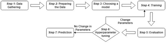

Disclaimer/Publisher’s Note: The statements, opinions and data contained in all publications are solely those of the individual author(s) and contributor(s) and not of MDPI and/or the editor(s). MDPI and/or the editor(s) disclaim responsibility for any injury to people or property resulting from any ideas, methods, instructions or products referred to in the content. |
© 2026 by the authors. Licensee MDPI, Basel, Switzerland. This article is an open access article distributed under the terms and conditions of the Creative Commons Attribution (CC BY) license.