Adaptive LASSO-MGARCH for Multivariate Volatility Forecasting

Abstract

This paper evaluates an Adaptive LASSO-MGARCH model for multivariate volatility forecasting, with applications in green and conventional bonds, equities, energy commodities, and EU carbon allowances. By introducing coefficient-specific adaptive penalisation directly into the multivariate GARCH variance equations, the model delivers a sparse and data-driven volatility spillover structure while preserving the positive definiteness of the conditional covariance matrix. Using daily data on green and conventional bonds, equities, energy commodities, and carbon allowances, we show that adaptive regularisation substantially reduces model complexity and improves economic interpretability relative to an unpenalised MGARCH benchmark. Out-of-sample forecasting experiments at multiple horizons demonstrate that the Adaptive LASSO-MGARCH model consistently achieves lower covariance forecast losses, and statistical tests based on the White reality check confirm that these improvements are significant across alternative loss functions.

1. Introduction

Understanding how volatility is transmitted across financial markets is central to risk management, asset allocation, and financial stability analysis. Multivariate GARCH (MGARCH) models provide a natural framework for this task because they model time-varying variances and covariances jointly, allowing volatility shocks in one market to propagate to others [1,2,3]. In applications where portfolios span heterogeneous assets, such as bonds, equities, energy commodities, and carbon permits, accurate covariance forecasts are particularly valuable because they directly determine hedge ratios, portfolio risk, and stress test outcomes.

A persistent challenge is that standard MGARCH specifications become difficult to estimate and to forecast as the cross-sectional dimension grows. Unrestricted multivariate variance dynamics typically involve $\mathcal{O}\left(N^2\right)$ parameters (although our empirical application considers $N=8$ assets, the unrestricted MGARCH variance equations are still parameter-rich due to their numerous cross-market terms; thus, “high-dimensional” here refers to the dimensionality of the parameter space rather than N alone), which can lead to overfitting and unstable forecasts in realistic sample sizes [3,4,5,6,7]. At the same time, the conditional covariance matrix must remain positive definite at all dates, otherwise likelihood evaluation and inference break down [2]. The literature has proposed several solutions, but each comes with trade-offs. The BEKK family ensures positive definiteness by construction [2], yet it remains parameter-heavy and quickly becomes computationally burdensome in systems beyond a handful of assets [3]. Constant conditional correlation (CCC) models reduce dimensionality by separating univariate variances from correlation dynamics [8,9], but flexible variants either impose strong homogeneity restrictions or reintroduce high-dimensional parameterisation when correlations are allowed to undertake rich interactions [6,7,10,11]. Factor-based MGARCH models achieve parsimony by attributing co-movement to a small set of latent drivers [3,12]. Still, they rely on strong structural assumptions that can be restrictive when dependence patterns are heterogeneous across markets.

Related work has therefore explored dimension-reduction and regularisation strategies for multivariate volatility models, aiming to control parameter proliferation and improve out-of-sample covariance forecasting. In particular, $L_1$-type penalisation has been used to promote sparse spillover structures in multivariate GARCH settings, reducing estimation noise and enhancing interpretability [4,7,13]. Forecast evaluations of multivariate volatility models are commonly conducted using loss functions designed for covariance matrices, and systematic comparisons highlight that gains in parsimony can translate into forecast improvements when models are assessed out of sample [14,15].

This paper adopts a complementary approach: rather than imposing strong ex ante restrictions on the transmission structure, we allow the data to determine which volatility spillover channels are economically and statistically relevant. Specifically, we propose an Adaptive-Lasso MGARCH model that introduces coefficient-specific $L_1$ penalisation into the multivariate variance equations. Regularisation methods are well established in statistics and machine learning as tools for controlling complexity and improving out-of-sample performance [16,17]. In econometrics, uniform LASSO penalties have been applied to multivariate volatility models to promote sparsity [4,7,18,19], but uniform penalisation can overshrink economically important coefficients and may induce non-negligible bias. The adaptive LASSO of Zou [20] addresses this issue by weighting the penalty term using preliminary estimates, penalising small coefficients strongly while shrinking large coefficients less. This preserves the computational advantages of convex $L_1$ regularisation and, under suitable conditions, is known to deliver selection consistency and oracle-type behaviour in the adaptive LASSO literature under suitable regularity conditions [20,21,22]. These properties are attractive in MGARCH settings where many cross-market links are plausibly weak, while a small subset may be persistent and forecast-relevant.

Our modelling choice combines adaptive regularisation with a CCC decomposition of the conditional covariance matrix. The CCC structure preserves positive definiteness by construction and isolates the high-dimensional component to the variance equations, where sparsity is directly imposed. The resulting framework produces (i) a parsimonious and interpretable volatility-spillover structure and (ii) covariance forecasts that are less sensitive to estimation noise than dense MGARCH benchmarks.

We apply the proposed AL-MGARCH to an eight-asset system spanning green and conventional bonds, global equities and green equities, energy commodities (oil, gas, coal), and carbon permits (EUAs). This system is economically relevant for studying transition-related risk because it links financial markets that respond to climate policy, energy-price shocks, and global risk appetite. The empirical analysis is designed to address the paper’s central question: Does adaptive regularisation improve multivariate covariance forecasting relative to standard MGARCH?

Related to the present study, Xu et al. [23] propose an Adaptive LASSO-MGARCH framework for high-dimensional multivariate volatility modelling and demonstrate its ability to recover sparse volatility spillover structures across financial markets. Their analysis primarily focuses on structural interpretation and in-sample transmission mechanisms, while the out-of-sample predictive performance of the Adaptive-Lasso MGARCH model is not formally evaluated. The current paper complements and extends this line of research by shifting the emphasis toward forecasting performance. We conduct a systematic out-of-sample comparison between AL-MGARCH and a standard MGARCH benchmark across multiple forecast horizons using statistically validated loss-based criteria. This allows us to assess whether the theoretical advantages of adaptive regularisation, namely sparsity, reduced estimation noise, and oracle-type behaviour, translate into economically meaningful gains in covariance forecasting accuracy. Hence, while Xu et al. [23] establish the modelling framework and its spillover implications, this paper provides the first dedicated evidence on its forecasting effectiveness. A concise comparison between the two papers is provided in Appendix A.

The main findings are threefold. First, the Adaptive-Lasso selects a sparse set of volatility-transmission channels, shrinking many cross-effects to exactly zero while retaining economically meaningful persistence and spillovers. Second, model selection through out-of-sample tuning yields a substantially lower information criterion relative to the unpenalised benchmark, consistent with the improved fit after accounting for complexity. Third, and most importantly, AL-MGARCH delivers more accurate out-of-sample covariance forecasts than MGARCH at daily, weekly, and monthly horizons under both statistical and economic loss functions; the improvements are statistically supported using the White [24] reality check.

The remainder of the paper is organised as follows. Section 2 introduces the MGARCH benchmark and the Adaptive-Lasso extension, and describes the estimation and multi-step forecasting. Section 3 summarises the data. Section 4 reports the estimation results and the out-of-sample forecasting comparison. Section 5 concludes.

2. Adaptive-Lasso MGARCH Model

2.1. Baseline Specification

Let ${\mathbf{r}}_t$ be the $N\times 1$ vector of demeaned daily asset returns and let ${\mathcal{F}}_{t-1}$ denote the information set available at time $t-1$. We consider a constant conditional correlation (CCC) MGARCH model in which

$${\mathbf{r}}_t={\mathit{\epsilon }}_t,{\mathit{\epsilon }}_t={\mathbf{D}}_t{\mathbf{e}}_t,$$

(1)

where ${\mathbf{D}}_t=\mathrm{diag}(h_{1t}^{1/2},\dots ,h_{Nt}^{1/2})$ and ${\mathbf{e}}_t\mid {\mathcal{F}}_{t-1}\sim \mathcal{N}(\mathbf{0},\mathbf{P})$. The constant correlation matrix is $\mathbf{P}=\left\{{\rho }_{ij}\right\}$ with ${\rho }_{ii}=1$. Hence, $\mathbb{E}({\mathit{\epsilon }}_t\mid {\mathcal{F}}_{t-1})=\mathbf{0}$ and

$$\mathbb{E}({\mathit{\epsilon }}_t{\mathit{\epsilon }}_t^{\prime }\mid {\mathcal{F}}_{t-1})={\mathbf{H}}_t={\mathbf{D}}_t\mathbf{P}{\mathbf{D}}_t.$$

Under CCC, ${\mathbf{H}}_t$ is positive definite if $\mathbf{P}$ is positive definite and the diagonal elements of ${\mathbf{D}}_t$ are strictly positive. In our implementation, $\mathbf{P}$ is estimated as the correlation matrix of standardized residuals, and is therefore positive semidefinite by construction, and the variance recursion is implemented with positivity constraints on $h_{it}$. We adopt CCC to guarantee positive definiteness and to keep the focus on improving high-dimensional variance estimation; the same variance-regularisation approach can be combined with time-varying correlation models, for example, DCC, in a straightforward extension.

Conditional variances follow a first-order multivariate GARCH recursion:

$${\mathbf{h}}_t=\mathit{\omega }+\mathbf{A}{\mathit{\epsilon }}_{t-1}^2+\mathbf{B}{\mathbf{h}}_{t-1},$$

(2)

where ${\mathbf{h}}_t={(h_{1t},\dots ,h_{Nt})}^{\prime }$, $\mathit{\omega }>0$, and $\mathbf{A},\mathbf{B}\in {\mathbb{R}}^{N\times N}$. Stationarity requires $\rho (\mathbf{A}+\mathbf{B})<1$, where $\rho (·)$ denotes the spectral radius, that is, the largest modulus of the eigenvalues.

2.2. Quasi-Maximum Likelihood Estimation

Under the Gaussian quasi-likelihood, the time-t log-density of ${\mathit{\epsilon }}_t$ is

$$logf({\mathit{\epsilon }}_t\mid \mathit{\theta })=-{\displaystyle \frac{N}{2}}log\left(2\pi \right)-{\displaystyle \frac{1}{2}}log\left|{\mathbf{H}}_t\right|-{\displaystyle \frac{1}{2}}{\mathit{\epsilon }}_t^{\prime }{\mathbf{H}}_t^{-1}{\mathit{\epsilon }}_t,$$

(3)

where $\mathit{\theta }$ collects the parameters in $(\mathit{\omega },\mathbf{A},\mathbf{B},\mathbf{P})$. The negative average log-likelihood is

$${\ell }_T\left(\mathit{\theta }\right)=-{\displaystyle \frac{1}{T}}{\displaystyle \sum _{t=1}^T}logf({\mathit{\epsilon }}_t\mid \mathit{\theta }).$$

(4)

The QMLE is $\widehat{\mathit{\theta }}=arg{min}_{\mathit{\theta }\in \Theta }{\ell }_T\left(\mathit{\theta }\right)$. In practice, $\mathbf{P}$ is estimated from standardized residuals ${\widehat{\mathbf{e}}}_t={\widehat{\mathbf{D}}}_t^{-1}{\widehat{\mathit{\epsilon }}}_t$ as $\widehat{\mathbf{P}}=\mathrm{corr}\left({\widehat{\mathbf{e}}}_t\right)$.

2.3. Adaptive-Lasso Regularisation

With unrestricted $\mathbf{A}$ and $\mathbf{B}$, the number of parameters grows on the order of $N^2$, and many cross-effects may be weak. To obtain a parsimonious variance transmission structure, we estimate a penalised version of the Gaussian QML objective:

$$\widehat{\mathit{\theta }}\left({\lambda }_T\right)=arg\underset{\mathit{\theta }\in \Theta }{min}\left\{{\ell }_T\left(\mathit{\theta }\right)+{\lambda }_T{\displaystyle \sum _{j=1}^d}{w}_j\left|{\theta }_j\right|\right\},$$

(5)

where ${\lambda }_T\ge 0$ is the shrinkage parameter and $w_j$ are adaptive weights. We set $w_j=1/max\left\{\right|{\tilde{\theta }}_j|,{ϵ}_w\}$, where ${\theta }_j$ is the jth element of the preliminary estimate $\tilde{\mathit{\theta }}$. We use a small constant ${ϵ}_w$ to avoid division by zero, and set ${ϵ}_w=0.005$ following Cattivelli and Gallo [25].

The AL-MGARCH estimator is obtained in three sequential steps.

1.

Initial QML: Estimate an unrestricted CCC-MGARCH(1,1) on the full sample and collect $\tilde{\mathit{\theta }}=(\tilde{\mathit{\omega }},\tilde{\mathbf{A}},\tilde{\mathbf{B}})$. Adaptive weights are then defined as

$$w_j=1/max\left\{\right|{\tilde{\theta }}_j|,{ϵ}_w\},{ϵ}_w=0.005,$$

The value of ${ϵ}_w$ is chosen following Audrino and Knaus [26] and Cattivelli and Gallo [25].

2.

Selection of the shrinkage parameter ${\widehat{\lambda }}_T$: Using only the first $2T/3$ observations, solve the penalised problem (5) over a grid of $n_{\lambda }=30$ equally spaced values ${\left\{{\lambda }_k\right\}}_{k=1}^{n_{\lambda }}\subset [{\lambda }_{max}/n_{\lambda },{\lambda }_{max}]$, where

$${\lambda }_{max}={\displaystyle \frac{|{\ell }_T\left(\tilde{\mathit{\theta }}\right)|}{Tdv}},d=2N^2+N.$$

We set $v=10$ following Cattivelli and Gallo [25]. For each ${\lambda }_k$, produce one-step forecasts on the hold-out sample ($T/3$ observations) and compute the QLIK loss [27]

$${\mathrm{QLIK}}_k={\displaystyle \sum _{t=T-T/3+1}^T}\left\{tr\left[{\left({\widehat{\mathbf{H}}}_{t|t-1}^{\left(k\right)}\right)}^{-1}{\mathbf{H}}_t\right]+log\left|{\widehat{\mathbf{H}}}_{t|t-1}^{\left(k\right)}\right|\right\}.$$

(6)

Choose ${\widehat{\lambda }}_T=arg{min}_k{\mathrm{QLIK}}_k$. A BIC or economic-loss criterion is also admissible; see [28].

3.

Adaptive-Lasso estimation: Re-estimate (5) on the full sample with ${\lambda }_T={\widehat{\lambda }}_T$, yielding ${\widehat{\mathit{\theta }}}_{{\widehat{\lambda }}_T}$.

Under standard regularity conditions (e.g., strict stationarity and finite fourth moments) and an appropriate penalty sequence, the AL-MGARCH estimator is selection-consistent and asymptotically normal. See Appendix B for details on the asymptotic properties.

2.4. Multi-Step-Ahead Covariance Forecasts

Under CCC, the s-step-ahead covariance forecast is

$${\widehat{\mathbf{H}}}_{t+s\mid t}={\widehat{\mathbf{D}}}_{t+s\mid t}\mathbf{P}{\widehat{\mathbf{D}}}_{t+s\mid t},{\widehat{\mathbf{D}}}_{t+s\mid t}=\mathrm{diag}\left({\widehat{\mathbf{h}}}_{t+s\mid t}^{1/2}\right).$$

(7)

From (2), the one-step variance forecast is

$${\widehat{\mathbf{h}}}_{t+1\mid t}=\mathit{\omega }+\mathbf{A}{\mathit{\epsilon }}_t^2+\mathbf{B}{\mathbf{h}}_t.$$

(8)

For $s\ge 2$, ${\mathit{\epsilon }}_{t+s-1}^2$ is unobserved at time t and is replaced by its conditional expectation, and

$$\mathbf{C}=\mathbf{A}+\mathbf{B},$$

(9)

The variance forecasts satisfy

$${\widehat{\mathbf{h}}}_{t+s\mid t}=\mathit{\omega }+\mathbf{C}{\widehat{\mathbf{h}}}_{t+s-1\mid t},s\ge 2.$$

(10)

Solving recursively gives the closed-form expression

$${\widehat{\mathbf{h}}}_{t+s\mid t}={\tilde{\mathit{\omega }}}_s+{\mathbf{C}}^{s-1}{\widehat{\mathbf{h}}}_{t+1\mid t},{\tilde{\mathit{\omega }}}_s={(\mathbf{I}-\mathbf{C})}^{-1}(\mathbf{I}-{\mathbf{C}}^{s-1})\mathit{\omega },$$

(11)

for $\rho \left(\mathbf{C}\right)<1$. Equations (7)–(11) define the s-step-ahead covariance forecasts used below.

3. Data

We study an eight-asset system designed to capture volatility transmission across (i) fixed income (green and conventional bonds), (ii) energy and commodity markets (Brent crude, natural gas, coal), (iii) carbon pricing (EU Emissions Allowances), and (iv) global equities (broad market and green/ESG equities). All series are daily close-to-close prices in USD (or USD-hedged for AGGB). Returns are log-differences multiplied by 100.

Green bonds are proxied by the Solactive Green Bond Index (GBOND). Conventional bonds are proxied by the USD-hedged Bloomberg Global Aggregate Bond Index (AGGB). Energy commodities include Brent crude futures (BRENT), thermal coal (COAL), and natural gas (GAS). Carbon risk is captured by the EU Emissions Allowances (EUA). Global equity risk is represented by MSCI ACWI (STOCK) and green equities by the MSCI Global Environment Index (ESG).

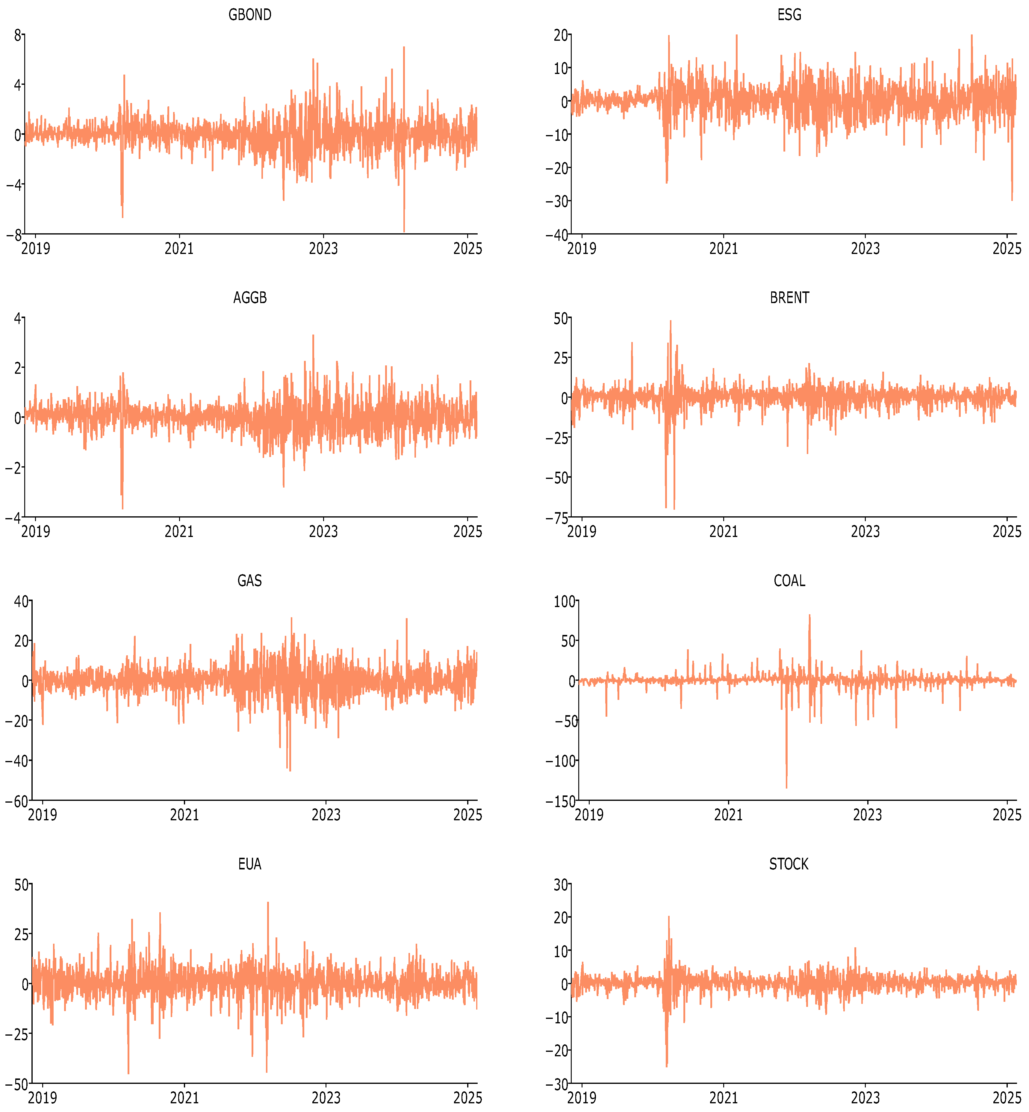
The sample spans January 2018 to June 2025 with T = 1509 observations, which is the longest common window across all series. Additional details on the data sources, sample construction, and code implementation are provided in the Supplementary Materials. Figure 1 plots daily log-returns for the eight assets over the common sample (January 2018–June 2025).

Figure 1 plots daily log-returns for the eight assets over the common sample (January 2018–June 2025). The sample is constructed as the longest overlapping window across all series; if any asset is missing on a given trading day, that date is removed for all assets to maintain a balanced panel. The figure also highlights several notable volatility episodes. Volatility rises sharply during the March 2020 COVID-19 sell-off across bonds, equities, EUA and Brent, while GAS and COAL are comparatively less affected. From mid-2021, EUA enters a persistent high-volatility phase, and from February 2022 GAS and COAL display pronounced swings around the Russia–Ukraine energy shock. We retain these observations unchanged (i.e., no trimming or winsorisation), as they reflect the economically meaningful shocks that the model is designed to capture.

Table 1. Descriptive statistics of daily log-returns.

	GBOND	ESG	AGGB	BRENT	GAS	COAL	EUA	STOCK
Min	−7.874	−24.843	−13.95	−70.50	−51.553	−135.294	−49.022	−25.192
Max	7.010	37.313	6.03	48.075	31.369	82.206	40.802	20.308
Mean	0.001	0.095	−0.03	0.036	−0.090	0.019	0.333	0.086
Std	1.193	4.764	0.90	6.613	7.116	8.046	7.464	2.643
Skew	−0.261	−0.001	−2.76	−1.344	−0.353	−2.606	−0.333	−1.059
Kurt	8.507	7.720	42.60	21.771	6.920	69.350	7.372	17.253
LB2	312.148	251.603	10.501	435.717	398.796	59.899	213.785	1581.352

Note. GBOND: Solactive Green Bond Index; ESG: MSCI Global Environment index; AGGB: USD-hedged Bloomberg Global Aggregate; BRENT: ICE Brent Crude futures contract front-month; GAS: S&P GSCI 3-Month Forward Natural Gas Index (ER); COAL: ICE Rotterdam coal nearby; EUA: EU Emissions Allowances (EEX EUA); STOCK: MSCI All-Country World Index. LB² is the Ljung–Box statistic for squared returns at lag 20; the 5% critical value is 31.41.

reports descriptive statistics. It reveals three stylised facts. First, at the mean level, most series are mean-reverting around zero: EU Emission Allowances (EUA) are the only asset with a significant positive drift (0.333), while the green equity index (ESG, 0.095) and the conventional equity index (STOCK, 0.086) show merely modest upticks. By contrast, natural gas records a small negative drift (GAS, −0.09), reflecting the prolonged weakness in global gas prices. The aggregate bond index (AGGB, −0.03) also trends slightly downward, consistent with the post-2017 ‘repricing of duration’ triggered by rising long-term yields. Second, volatility varies widely across markets. The standard deviations of crude oil (6.613) and natural gas (7.116) are more than six times that of conventional bonds (AGGB, 0.9), with green bonds (GBOND, 1.193) sitting in between. This pattern aligns with the summary statistics reported in Reboredo et al. [29] and Mensi et al. [30]. Third, all distributions deviate from normality. Every asset shows negative skewness, reflecting frequent downside moves, and kurtosis is far above the Gaussian benchmark of three, reaching 42.6 for conventional bonds and 69.3 for coal. These results indicate fat tails and sharp peaks, characteristic of heavy-tailed behaviour. The Ljung–Box statistics for squared returns (lag 20) are highly significant in every column, confirming pronounced ARCH effects and justifying the use of an MGARCH specification in the subsequent analysis.

4. Empirical Results

This section evaluates the proposed Adaptive-Lasso MGARCH (AL-MGARCH) model. We first report the benchmark MGARCH(1,1) estimates, then show how the Adaptive-Lasso delivers a more parsimonious volatility-transmission structure, and finally assess whether this parsimony translates into better out-of-sample covariance forecasts.

4.1. MGARCH Benchmark

We use an unrestricted CCC–MGARCH(1,1) as the benchmark because it is the standard baseline specification and provides a direct dense-versus-sparse comparison under identical variance dynamics.

Table 2. MGARCH estimates of the coefficient matrices $\mathbf{A}$ and $\mathbf{B}$.

	GBOND	ESG	AGGB	BRENT	GAS	COAL	EUA	STOCK
Matrix $\mathbf{A}$
GBOND	0.1128	0.0315	0.0850	−0.0053	0.0430	−0.0041	0.0136	0.0152
ESG	0.0207	0.1128	0.0184	0.0003	−0.0161	−0.0059	−0.0063	0.0042
AGGB	0.0574	−0.0005	0.1598	−0.0006	0.0603	−0.0029	−0.0119	0.0343
BRENT	−0.0021	−0.0018	0.0173	0.1109	0.0123	0.0113	0.0062	0.0426
GAS	0.0261	−0.0203	0.0078	−0.0004	0.1298	−0.0018	−0.0045	0.0102
COAL	0.1015	−0.0238	−0.0686	−0.0021	0.1373	0.0774	−0.0061	−0.0007
EUA	0.0202	0.0083	−0.0199	0.0077	0.0110	0.0085	0.1161	0.0430
STOCK	0.0200	−0.0063	−0.0232	0.0038	0.0169	−0.0015	0.0166	0.1723
Matrix $\mathbf{B}$
GBOND	0.5193	0.0837	0.0413	−0.0091	0.0885	0.0509	0.0337	−0.0150
ESG	−0.0110	0.8306	−0.0356	−0.0211	0.0597	0.0221	−0.0022	0.0215
AGGB	0.0532	0.0193	0.4764	−0.0141	0.0929	0.0437	−0.0306	−0.0170
BRENT	−0.0180	−0.0098	0.0114	0.7644	−0.0410	0.0012	−0.0185	0.0491
GAS	−0.0166	0.0656	−0.0186	0.0104	0.8156	0.0002	0.0143	−0.0375
COAL	−0.0001	0.0234	0.0047	0.0203	0.1282	0.5480	0.0319	−0.0311
EUA	−0.0030	−0.0056	−0.0307	−0.0140	0.0225	−0.0129	0.7412	0.0155
STOCK	0.0018	0.0574	−0.0041	0.0418	−0.0098	−0.0024	−0.0168	0.7133
Log-likelihood: 10.2094
BIC: 916.4390

Notes: Bold entries indicate statistical significance at the 5% level. Log-likelihood and Bayesian Information Criterion (BIC) are reported at the bottom of the table. BIC uses active (nonzero) coefficients as effective degrees of freedom.

reports the unrestricted MGARCH(1,1) estimates (all estimations were conducted in Matlab R2024a using the fmincon optimisation routine).

The diagonal elements of $\mathbf{A}$ and $\mathbf{B}$ are sizeable across assets, confirming strong own-market volatility feedback and persistence. A number of off-diagonal coefficients are also statistically significant, indicating that volatility shocks can propagate across markets (bonds, energy commodities, carbon permits, and equities). The unrestricted MGARCH benchmark produces a dense volatility-transmission structure. In our eight-asset system, approximately 37% of the off-diagonal elements in the $\mathbf{A}$ and $\mathbf{B}$ matrices are statistically significant at the 5% level, implying widespread cross-market volatility interactions. While this richness may appear desirable from a structural perspective, it comes at a cost for forecasting. A dense parameterisation forces the model to estimate many small but persistent cross-effects, which are often weakly identified and sensitive to sampling variation. As a result, these nonzero coefficients may primarily reflect estimation noise rather than stable economic linkages, leading to overfitting and reduced out-of-sample performance.

4.2. Adaptive-Lasso MGARCH: Sparse Transmission and Improved Fit

Our main contribution is to regularise the MGARCH variance dynamics using the Adaptive Lasso, which selects a sparse set of economically relevant volatility spillover channels while shrinking weak cross-effects exactly to zero. The shrinkage parameter ${\lambda }_T$ is selected using a rolling validation scheme: the estimation window is split into a training subsample used for tuning ${\lambda }_T$ and a validation subsample used to minimise one-step-ahead forecast loss. Specifically, the first 1000 observations are used as the training subsample to construct the adaptive weights and estimate the model for a given ${\lambda }_T$, while the last 509 observations form the validation subsample used to select ${\widehat{\lambda }}_T$ by minimising one-step-ahead QLIK. The penalised model is then re-estimated on the full sample at the optimal ${\widehat{\lambda }}_T$.

Table 3. Adaptive-Lasso estimates of the coefficient matrices $\mathbf{A}$ and $\mathbf{B}$.

	GBOND	ESG	AGGB	BRENT	GAS	COAL	EUA	STOCK
Matrix $\mathbf{A}$
GBOND	0.1518	0.0104	0.0858	0	0.0123	−0.0028	−0.0011	0.0045
ESG	0.0012	0.1677	0.0041	0	0.0019	0	0	0.0015
AGGB	0.0181	0	0.2377	0	−0.0011	0	−0.0031	0.0125
BRENT	0.0013	0	0	0.1691	0	0	0	−0.0011
GAS	0.0069	−0.0029	0	0	0.2326	0.0019	0	0.0014
COAL	0.0508	−0.0130	−0.0672	0.0017	0.1900	0.1293	0	0
EUA	0.0026	0.0026	0.0059	−0.0045	0.0011	0.0025	0.1623	0
STOCK	−0.0056	0	0	−0.0111	−0.0022	−0.0012	0.0036	0.2370
Matrix $\mathbf{B}$
GBOND	0.5964	0.0145	0.0562	0.0072	0.0256	0.0401	−0.0042	0.0081
ESG	0	0.7897	−0.0020	0.0030	0.0408	0.0020	0	−0.0056
AGGB	0.0135	−0.0042	0.5944	0.0022	0.0641	−0.0117	−0.0099	−0.0023
BRENT	0	−0.0023	−0.0014	0.7497	−0.0046	0	0.0178	0.0289
GAS	0	−0.0104	0	0.0040	0.6914	0	−0.0064	0
COAL	0	0	0	0	0.1430	0.4911	−0.0015	0
EUA	0	0	−0.0047	0.0032	−0.0021	−0.0041	0.6680	0
STOCK	0.0016	0.0034	0	0.0080	0.0016	0	−0.0015	0.7290
Log-likelihood: 11.2304
BIC: 636.2674

Note: Elements set exactly to zero by the penalty appear as “0”. Standard errors (or t-ratios) are available upon request. BIC uses active (nonzero) coefficients as effective degrees of freedom.

reports the resulting Adaptive-Lasso estimates. Relative to the dense MGARCH benchmark, the coefficient matrices become markedly sparse, particularly in off-diagonal elements. In the short-run shock matrix $\mathbf{A}$, the largest surviving coefficients are concentrated on the diagonal, while only a limited number of cross-market effects remain, indicating that immediate volatility transmission is confined to a small subset of markets. By contrast, in the persistence matrix $\mathbf{B}$, diagonal elements remain large, and several cross-market channels survive, suggesting that volatility spillovers are more pronounced at longer horizons than at the daily impact horizon.

This sparsity yields a parsimonious and interpretable volatility-transmission structure and substantially reduces effective model complexity. Consistent with this interpretation, the AL-MGARCH attains a higher log-likelihood and a substantially lower BIC than the unpenalised MGARCH. Here, BIC is computed using the number of active (nonzero) penalised coefficients as effective degrees of freedom, so it should be interpreted as a fit–parsimony trade-off under regularisation. Together with its superior out-of-sample forecasting performance, these results indicate that the reduction in estimation variance achieved through adaptive regularisation dominates any bias introduced by shrinkage, leading to improved generalisation.

4.3. Out-of-Sample Forecasting Comparison

The central empirical question is whether the proposed AL-MGARCH improves predictive performance relative to the unrestricted MGARCH benchmark. We therefore compare out-of-sample forecasts of the conditional covariance matrix at horizons $h\in \{1,5,22\}$ trading days (daily, weekly, and monthly horizons). Forecast accuracy is evaluated using two standard statistical loss functions for covariance forecasts: QLIK and FN (Frobenius norm). Realised covariance is proxied by ${\mathbf{RC}}_t={\mathbf{r}}_t{\mathbf{r}}_t^{\prime }$. See [27,28] for the details of the two loss functions.

Forecasts are generated in a rolling-window design: each model is re-estimated every fifth observation using a rolling window of 1000 observations, and h-step-ahead covariance forecasts are produced recursively for $h>1$. To test whether forecast improvements are statistically meaningful, we apply the White [24] reality check based on the stationary bootstrap of Politis and Romano [31].

Table 4. Out-of-sample forecasting performance: statistical loss functions.

Horizon	QLIK		FN
	AL-MGARCH	MGARCH	AL-MGARCH	MGARCH
$h=1$	4.4026	4.5574	7.9173	7.9591
$h=5$	4.9232	5.1342	7.9569	7.9954
$h=22$	5.9333	6.1867	8.0863	8.1516

Note: Bold indicates significance at the 5% level based on the White (2000) [24] reality check.

reports average out-of-sample losses. Across all horizons and both loss functions, AL-MGARCH yields lower losses than MGARCH. The gains are present at the one-step horizon and persist at longer horizons, which is consistent with the motivation for regularisation: by eliminating weak and unstable spillover coefficients, AL-MGARCH improves generalisation and delivers more accurate covariance forecasts. In sum, the results provide empirical support for the proposed AL-MGARCH framework as a practical alternative to dense MGARCH specifications when the cross-sectional dimension is moderate and forecasting performance is the primary objective.

The economic loss functions are relevant for evaluating covariance matrix forecasts, as they are based on forecasted portfolio performance. The same economic loss functions as in [32] are used, namely the global minimum variance portfolio (GMV) and the minimum variance portfolio (MV); see also [27,28]. These loss functions are the variances in the forecasts of portfolio returns. Given a covariance matrix forecast $H_{t+s|t}^a$, the GMV portfolio weight vector $w_{t+s}^a$ is computed as the minimizer of the portfolio variance ${\left(w_{t+s}^a\right)}^{\prime }{H}_{t+s|t}^a{w}_{t+s}^a$ subject to the constraint that the weights add to unity. Next the portfolio return $w_{t+s}^a{r}_{t+s}$ is computed. Once this procedure is carried out for each forecast date, the variance in the resulting time series of optimal portfolio returns is used as the loss function in the MCS procedure, since a superior model produces optimal portfolios with lower forecast variance.

The MV portfolio is obtained by minimising the portfolio variance subject to the additional constraint that the expected portfolio return be larger than a chosen value. Following Engle and Kelly [32], this value is fixed at 10% and the expected portfolio return at the mean of the data.

Table 5. Out-of-sample forecasting performance: economic loss functions.

Horizon	GMV			MV
	AL-MGARCH	MGARCH	Impr. (%)	AL-MGARCH	MGARCH	Impr. (%)
$h=1$	1.261	1.382	8.76	2.241	2.452	8.61
$h=5$	1.334	1.456	8.38	2.352	2.567	8.38
$h=22$	1.402	1.524	8.01	2.437	2.583	5.65

Note: Impr. (%) is the percentage reduction in loss relative to MGARCH, $(\mathrm{MGARCH}-\mathrm{AL}\text{-}\mathrm{MGARCH})/\mathrm{MGARCH}\times 100$. Bold indicates significance at the 5% level based on the White (2000) [24] reality check.

reports the out-of-sample economic loss functions based on portfolio variance for the global minimum variance (GMV) and mean-variance (MV) portfolios. In both cases, the loss corresponds to the realised variance in the optimal portfolio returns constructed using the forecasted covariance matrix. Lower values therefore indicate superior economic performance, as they imply more stable portfolios and improved risk control.

Across all forecast horizons ($h=1,5,22$), the AL-MGARCH model consistently delivers lower portfolio variance than the benchmark MGARCH model for both portfolio strategies. For the GMV portfolio, the variance reductions are economically meaningful and statistically significant at the 5% level according to the White [24] reality check. For instance, at the one-day horizon, the GMV variance decreases from 1.382 under MGARCH to 1.261 under AL-MGARCH, corresponding to an approximate 9% reduction in realised portfolio risk. Similar improvements persist at the weekly ($h=5$) and monthly ($h=22$) horizons, indicating that the gains from sparse covariance estimation remain robust over longer investment horizons.

The economic gains are even more pronounced for the constrained MV portfolio, which incorporates a minimum expected return requirement. At all horizons, AL-MGARCH achieves substantially lower portfolio variance than MGARCH, with statistically significant improvements. This suggests that adaptive regularisation improves not only statistical forecast accuracy but also portfolio risk performance under constraints—an implication that is broadly relevant for global institutional investors and risk managers, with particular salience for those exposed to Europe’s carbon and energy markets (e.g., EUAs).

Overall, these results confirm that the forecasting gains of AL-MGARCH are economically meaningful. By eliminating noisy and weak spillover channels, the adaptive penalisation delivers more stable covariance forecasts, leading to improved portfolio allocation and superior out-of-sample risk performance. The consistency of the results across portfolio objectives and forecast horizons strengthens the practical relevance of the proposed AL-MGARCH framework.

4.4. Robustness

A natural extension would be to assess robustness through dedicated subsample analysis and formal structural-stability tests. In this paper, however, the empirical design already relies on an out-of-sample rolling-window framework with a 1000-observation estimation window, with parameters re-estimated repeatedly over time. As such, forecasting performance is evaluated across many overlapping subsamples and changing market conditions, providing an informal assessment of stability.

The results show that AL-MGARCH consistently outperforms the unpenalised MGARCH benchmark across forecast horizons and evaluation criteria. This suggests that the improvement is not driven by a particular sample period. Since the main objective of the paper is to compare the out-of-sample forecasting performance of AL-MGARCH and MGARCH, we consider the rolling-window evidence sufficient for the present analysis. Nevertheless, explicit subsample splits and formal break or stability tests would be useful extensions for future research.

5. Conclusions

This paper proposes and evaluates an Adaptive LASSO-MGARCH framework for modelling and forecasting high-dimensional conditional covariance dynamics. By introducing coefficient-specific penalisation directly into the multivariate GARCH variance equations, the model delivers a sparse yet flexible representation of volatility spillovers while mitigating over-parameterisation and estimation noise.

An empirical application to a system of bond, equity, energy, and carbon markets shows that adaptive regularisation substantially simplifies the volatility transmission structure without sacrificing in-sample fit. More importantly, out-of-sample forecasting results demonstrate that AL-MGARCH consistently outperforms an unpenalised MGARCH benchmark across short-, medium-, and long-horizon covariance forecasts. These gains are statistically significant under multiple loss functions and remain robust to rolling-window re-estimation.

The AL-MGARCH framework therefore offers a practical and scalable tool for high-dimensional risk forecasting. Improved covariance forecasts translate into more stable risk estimates, hedge ratios, and portfolio weights. This is relevant for institutional investors (e.g., constrained minimum-variance allocation and risk management) and also for individual investors using risk-based allocation rules. The main practical benefit of AL-MGARCH is that it reduces estimation noise by shrinking weak spillover channels, leading to more robust covariance forecasts.

Our framework adopts a CCC decomposition, so correlation dynamics are not modelled explicitly; extending the approach to time-varying correlations (e.g., DCC-type models) is a natural next step. Future work could also incorporate asymmetric volatility effects and heavier-tailed innovations, and consider alternative realised covariance measures when higher-frequency data are available.