RBF Neural Network Fusion Disturbance Estimation for Robust Synchronization of Chaotic Systems

Abstract

This paper addresses the problem of complete synchronization of chaotic systems subject to external disturbances and parameter uncertainties, proposing a robust control strategy based on radial basis function (RBF) neural network fusion with a disturbance estimator (DE)-based control method. Firstly, a dynamic feedback controller is designed to stabilize the nominal error system. Subsequently, a set of appropriate filters are constructed, and based on these filters, a disturbance estimator that can asymptotically track external disturbances is developed, thereby realizing asymptotic cancelation of external disturbance effects on the synchronization process. Then, an RBF-based compensator is designed to approximate the unmodeled uncertainties of the system with high precision, effectively suppressing the adverse impacts of uncertainties. By integrating the aforementioned dynamic feedback controller, disturbance estimator, and RBF-based compensator, robust complete synchronization between the master and slave chaotic systems is successfully achieved. Finally, a numerical simulation example is presented to validate the feasibility and effectiveness of the proposed control scheme.

1. Introduction

The study of chaotic systems originated with Edward Lorenz’s discovery of the Lorenz system in the 1960s [1], a seminal contribution that fundamentally reshaped the understanding of nonlinear dynamics. Characterized by sensitive dependence on initial conditions, complex topological structures, and unpredictable long-term behavior, the Lorenz system catalyzed the emergence of chaos as a distinct and significant field of inquiry. Since then, chaotic systems and their associated control problems have become a central and highly active research direction within nonlinear control theory. This prominence stems largely from the ubiquity of chaotic phenomena across both natural and engineered systems, including meteorological processes [2], power grids [3], chemical reactions [4], and biological networks [5]. Among the various topics in chaos research, the complete synchronization of two identical chaotic systems has garnered particular attention and is widely regarded as a problem of fundamental importance (see Ref. [6]). Complete synchronization refers to the process by which the state trajectories of two chaotic systems converge to an identical motion under an appropriately designed control law. This problem is not only of great theoretical significance for deepening the understanding of complex dynamical behavior, but also holds substantial practical value due to its extensive applications in fields such as secure communication [7,8,9], image encryption [10], and industrial control [11,12]. To date, a considerable body of research has been devoted to the problem of chaotic synchronization, with notable contributions documented in Refs. [13,14,15,16,17,18] and the references therein.

In practical engineering applications, chaotic systems are frequently subject to external disturbances such as environmental noise, parameter fluctuations, and exogenous interference signals, which can destabilize the system and severely degrade the synchronization performance between master and slave systems. The uncertainty and disturbance estimator (UDE)-based control method has been widely recognized as an effective approach for handling such disturbances in nonlinear systems (see Refs. [19,20,21]), offering advantages including structural simplicity, ease of implementation, and no requirement for accurate mathematical models of disturbances. The core idea of the UDE-based control method is to lump system uncertainties and external disturbances into a single composite term, which is then asymptotically estimated through a suitably designed filter, with the negative of this estimate incorporated into the control law to counteract both uncertainties and disturbances. In contrast, the filter design approach proposed in Ref. [21] is based solely on external disturbances; consequently, the presence of system uncertainties compromises the estimation accuracy of the filter, preventing complete uncertainty cancelation and yielding only practical stability in a certain sense. Moreover, for a class of external disturbances comprising bounded trigonometric functions, Ref. [21] presents a second-order filter without accounting for the influence of frequency on estimation performance, whereas for trigonometric disturbances with different frequencies, the filter design should inherently be frequency-dependent, a key insight underlying the disturbance estimator (DE)-based control method. A notable limitation of the UDE-based approach is that the asymptotic estimation capability of the designed filter remains relatively limited, particularly for time-varying or complex disturbances, making it difficult to achieve complete disturbance cancelation. In recent years, the DE-based control method [22,23,24] has emerged as an enhanced alternative; by refining the filter structure and estimation mechanism, it improves both the accuracy and convergence rate of disturbance estimation, effectively addressing some shortcomings of the UDE-based method. Nevertheless, the DE-based method still exhibits a clear limitation in that it focuses exclusively on the estimation and compensation of external disturbances, while being incapable of effectively handling parameter uncertainties or unmodeled dynamics inherent to the system. If left unaddressed, these uncertainties can also lead to performance degradation in synchronization control; therefore, it becomes necessary to integrate the DE-based control method with other advanced control techniques to achieve comprehensive suppression of both disturbances and system uncertainties.

RBF neural networks have been widely used in nonlinear system control due to their excellent approximation capabilities, simple structures, and fast convergence speeds; see Refs. [25,26,27]. Unlike traditional linear approximation methods, RBF neural networks can approximate any continuous nonlinear function with arbitrary precision within a compact set by adjusting the weights and basis functions, which makes them particularly suitable for dealing with system uncertainties and unmodeled dynamics that are difficult to describe with accurate mathematical models. The approximation mechanism of RBF neural networks is based on the linear combination of radial basis functions centered at different nodes, which can adaptively learn the characteristics of nonlinear functions through training algorithms. Given the strong approximation ability of RBF neural networks and the excellent disturbance estimation performance of the DE-based control method, it is a natural and effective idea to integrate the DE-based control method with RBF neural networks to solve the synchronization problem of chaotic systems with both external disturbances and parameter uncertainties. This fusion strategy can give full play to the advantages of the two methods: the DE-based control method is responsible for accurately estimating and compensating for external disturbances, while the RBF neural network is used to approximate and suppress system uncertainties, thereby forming a complementary and robust control framework.

Based on the above discussions and analysis, this study focuses on the complete synchronization problem of a class of chaotic systems subject to external disturbances and parameter uncertainties and proposes a robust control strategy by combining the DE-based control method with an RBF neural network. First, aiming at the stability of the nominal error system, a dynamic feedback controller is designed to lay a solid foundation for subsequent synchronization control. Then, a set of dedicated filters are constructed, and a disturbance estimator based on these filters is developed to asymptotically track external disturbances, realizing the effective cancelation of disturbance effects. Meanwhile, an RBF-based compensator is designed to accurately approximate the parameter uncertainties and unmodeled dynamics of the system, thereby suppressing the adverse impacts caused by uncertainties. By integrating the dynamic feedback controller, disturbance estimator, and RBF-based compensator, the robust complete synchronization of master–slave chaotic systems is successfully achieved.

The main contributions of this paper are as follows:

• A dynamic feedback controller is designed to stabilize the nominal error system.
• A set of dedicated filters are constructed, and a disturbance estimator based on these filters is developed to asymptotically track external disturbances, realizing the effective cancelation of disturbance effects.
• In the previous literature, the model uncertainty and external disturbance are lumped together as a single term $U_d=g\left(x\right)+d\left(t\right)$, where $g\left(x\right)$ denotes the model uncertainty and $d\left(t\right)$ is the external disturbance. An appropriate filter $G_f\left(s\right)$ is then designed to estimate $U_d$; i.e., ${\widehat{U}}_d=U_d\ast {\mathcal{L}}^{-1}\left[G_f\left(s\right)\right]$ is used to approximate $U_d$. Since the filter $G_f\left(s\right)$ is designed based on $d\left(t\right)$, it is evident that, in general, ${\widehat{U}}_d$ cannot asymptotically approximate $U_d$ because the presence of $g\left(x\right)\ne 0$ compromises the estimation performance of the filter. To address this issue, this paper employs an RBF neural network to approximate $g\left(x\right)$. Accordingly, we define $\overline{d}\left(t\right)=g\left(x\right)-\widehat{g}\left(x\right)+d\left(t\right)$, where $u_{rbf}=-\widehat{g}\left(x\right)$ represents the designed RBF controller. Consequently, the estimate ${\widehat{\overline{U}}}_d=\widehat{d}\left(t\right)+\widehat{g}\left(x\right)=\left[g\left(x\right)-\widehat{g}\left(x\right)+d\left(t\right)\right]\ast {\mathcal{L}}^{-1}\left[G_f\left(s\right)\right]+\widehat{g}\left(x\right)$ achieves a significantly improved approximation of $U_d$.

Before concluding this section, we introduce some notations that will be used throughout the paper. Let i denote the imaginary unit, i.e., $i^2=-1$. The symbols “$\mathcal{L}$” and “${\mathcal{L}}^{-1}$” represent the Laplace transform and its inverse, respectively. For a function $h\left(t\right)$ satisfying appropriate conditions, its Laplace transform is defined as

$$H\left(s\right)=\mathcal{L}\left[h\left(t\right)\right]={\int }_0^{+\infty }h\left(t\right)e^{-st}dt,$$

where s is complex variable with $\mathrm{Re}\left(s\right)>0$ and $h\left(t\right)={\mathcal{L}}^{-1}\left[H\left(s\right)\right]$.

The symbol “*” denotes the convolution operation between two functions. For functions $h_1\left(t\right)$ and $h_2\left(t\right)$ satisfying suitable conditions, their convolution is given by

$$h_1\left(t\right)\ast h_2\left(t\right)={\int }_0^t{h}_1(t-\tau )h_2\left(\tau \right)d\tau .$$

2. Preliminary

Lemma 1

([21]). Consider the following nonlinear system

$$\dot{q}=H\left(q\right)+w\left(t\right)$$

(1)

where $q\in R^n$ represents the state variables and $w\left(t\right)\in R^n$ denotes the external disturbances. If the system $\dot{q}=H\left(q\right)$ is exponentially stable in large and $\parallel w\left(t\right)\parallel \le \lambda e^{-\alpha t}$, with $\lambda >0$ and $\alpha >0$ being a sufficiently large number, then it follows that ${\displaystyle \underset{t\to \infty }{lim}\parallel q\left(t\right)\parallel =0}$.

Lemma 2

([25]). Neural networks (NNs) have demonstrated remarkable capability in approximation, and they can mimic a continuous function $f\left(v\right):R^n\to R^m$ with the following expression within a compact set ${\mathrm{\Omega }}_v\subset R^n$:

$$f_{NN}\left(v\right)=W^{T}h\left(v\right)$$

(2)

where W represents the weights of the neural networks, belongs to $R^{p\times m}$ and corresponds to a certain number of neurons p, with $h\left(v\right)=$ ${[h_1\left(v\right),\dots ,h_p\left(v\right)]}^T$$\in R^p$, where $h_i\left(v\right)=exp(-{(v-{\tau }_i)}^T(v-{\tau }_i)/2{\mu }_i^2)\in R$ with the centers ${\tau }_i={[{\tau }_{i1},{\tau }_{i2},\dots ,{\tau }_{in}]}^T\in R^n$ and width ${\mu }_i\in R$.

3. Problem Formulation

Consider the following controlled chaotic system subject to external disturbances and parameter uncertainties:

$$\begin{array}{c}\hfill \dot{x}=f\left(x\right)+b\left[u+g\left(x\right)+d\left(t\right)\right]\end{array}$$

(3)

where $x\left(t\right)\in {\mathrm{R}}^n$ is the state variable, $f\left(x\right)\in {\mathrm{R}}^n$ is the continuous function, $b\in {\mathrm{R}}^{n\times 1}$ is a constant matrix, $g\left(x\right)\in \mathrm{R}$ is the uncertainty of the system (3), $u\in \mathrm{R}$ is the controller that needs to be designed, and $d\left(t\right)\in \mathrm{R}$ is the periodic disturbance, i.e.,

$$d\left(t\right)=psin\left({\omega }_{1}t\right)+qcos\left({\omega }_{2}t\right)+r$$

(4)

where p, q and r are unknown constants with $p^2+q^2+r^2\ne 0$; both ${\omega }_1$ and ${\omega }_2$ are frequencies, which are known in advance.

Let the system (3) be the master system, then the corresponding slave system is presented below

$$\begin{array}{c}\hfill \dot{y}=f\left(y\right)\end{array}$$

(5)

where $y\left(t\right)\in {\mathrm{R}}^n$ is the state variable and $f\left(y\right)\in {\mathrm{R}}^n$ is the continuous function.

In what follows, let $e=x-y$, then the error system is given as follows

$$\begin{array}{c}\hfill \dot{e}=F(x,e)+b\left[u+g\left(x\right)+d\left(t\right)\right]\end{array}$$

(6)

where $e\left(t\right)\in {\mathrm{R}}^n$ is the state variable and $F(x,e)=f\left(x\right)-f\left(y\right)$.

The main objective of this paper is to design a suitable controller

$$\begin{array}{c}\hfill u=u_c+u_{\mathrm{rbf}}+u_d\end{array}$$

(7)

to achieve the following control goal:

$$\begin{array}{c}\hfill \underset{t\to \infty }{lim}∥e\left(t\right)∥=0\end{array}$$

(8)

where $u_c$ ensures the following system

$$\begin{array}{c}\hfill \dot{e}=F(x,e)+b{u}_c\end{array}$$

(9)

is asymptotically stable with respect to origin, and system (9) is commonly referred to as the controlled nominal error system. $u_{\mathrm{rbf}}$ meets the following objective

$$\begin{array}{c}\hfill u_{\mathrm{rbf}}=-\widehat{g}\left(x\right)\to -g\left(x\right),\end{array}$$

(10)

$u_{\mathrm{rbf}}$ is called the uncertainty compensator which is applied to cancel the uncertainty with high precision. $u_d$ meets the following objective

$$\begin{array}{c}\hfill u_d=-\widehat{d}\left(t\right)=-\left[g\left(x\right)-\widehat{g}\left(x\right)+d\left(t\right)\right]\ast {\mathcal{L}}^{-1}\left[G_f\left(s\right)\right]\to -d\left(t\right), t\to +\infty ,\end{array}$$

(11)

$u_d$ is called the disturbance estimator which is used to asymptotically compensate for the disturbance and $G_f\left(s\right)$ is the designed filter.

4. Main Result

In this section, the stabilization of error system (6) is investigated using an RBF neural network fusion disturbance estimation method, which is implemented through three sequential steps. First, a dynamic feedback controller $u_c$ is proposed and adopted to stabilize nominal error system (9). In the second step, an RBF-based compensator $u_{\mathrm{rbf}}$ is designed to accurately approximate the uncertainties existing in the error system (6). Finally, several appropriate filters are constructed for the corresponding disturbances, and a disturbance estimator $u_d$ is developed to asymptotically track and compensate for these disturbances. Ultimately, a composite controller required for the system is formulated by integrating the design results of the above three steps, and it is applied to achieve the stabilization of error system (6).

For subsequent analysis and derivation, the following assumption is introduced:

Assumption 1.

Consider the uncontrolled error system (9), i.e., $\dot{x}=F(x,e)$, and suppose there exist positive definite matrices P and $Q_1$ such that

$$e^{T}PF(x,e)\le e^T{Q}_{1}e.$$

(12)

Remark 1.

In practice, condition (12) is not particularly restrictive; it is satisfied, for instance, when $f\left(x\right)$ is Lipschitz continuous. Specifically, the Lipschitz condition can be expressed as

$$\parallel F(x,e)\parallel =\parallel f\left(x\right)-f\left(y\right)\parallel \le \lambda \parallel x-y\parallel =\lambda \parallel e\parallel ,$$

(13)

where $\lambda >0$ is a constant.

Under the Lipschitz condition, it follows that

$$\parallel e^{T}PF(x,e)\parallel \le \parallel e^T\parallel \parallel P\parallel \parallel \lambda e\parallel ={\lambda \parallel P\parallel \parallel e\parallel }^2=e^T{Q}_{1}e,$$

Choosing $Q_1=\lambda \parallel P\parallel I$ (with I being the identity matrix of appropriate dimension) gives $e^T{Q}_{1}e={\lambda \parallel P\parallel \parallel e\parallel }^2$, and therefore

$$e^{T}PF(x,e)\le \parallel e^{T}PF(x,e)\parallel \le e^T{Q}_{1}e.$$

which establishes inequality (12).

4.1. Nominal Error System Stabilization

Theorem 1.

Consider the controlled nominal error system given by (9). If the pair $\left(F\right(x,e),b)$ is controllable, a stabilizing controller $u_c$ can be constructed as

$$u_c=k\left(t\right)b^{T}e\left(t\right)$$

(14)

where the dynamic feedback gain $k\left(t\right)$ is updated in accordance with the following adaptive law:

$$\dot{k}\left(t\right)=-e^{T}Pb{b}^{T}e$$

(15)

Proof. 

First, substituting the controller $u_c$ into system (9) yields

$$\begin{array}{c}\hfill \dot{e}=F(x,e)+k\left(t\right)b{b}^{T}e\end{array}$$

(16)

To analyze the stability of system (16), we introduce the following Lyapunov function candidate:

$$V_1\left(e\right)={\displaystyle \frac{1}{2}}{e}^{T}Pe+{\displaystyle \frac{1}{2}}{(k\left(t\right)+\overline{k})}^2$$

(17)

where $\overline{k}$ denotes a desired sufficiently small negative constant.

Computing the time derivative of $V_1\left(e\right)$ along the trajectory of system (15) and system (16), we have

$$\begin{array}{c}\hfill \begin{array}{ccc}{\dot{V}}_1\left(e\right)\hfill & =\hfill & e^{T}PF(x,e)+k\left(t\right)e^{T}Pb{b}^{T}e+(k+\overline{k})\dot{k}\left(t\right)\hfill \\ \hfill \\ \hfill & =\hfill & e^{T}PF(x,e)-\overline{k}{e}^{T}Pb{b}^{T}e\hfill \\ \hfill \\ \hfill & \le \hfill & e^T{Q}_{1}e-\overline{k}{e}^{T}Pb{b}^{T}e\hfill \\ \hfill \\ \hfill & =\hfill & e^T\left[Q_1-\overline{k}Pb{b}^T\right]e\hfill \\ \hfill \\ \hfill & =\hfill & -e^T{Q}_{2}e\hfill \end{array}\end{array}$$

(18)

where $Q_2=-\left[\overline{k}Pb{b}^T-Q_1\right]$ is a positive definite matrix.

Thus, ${\dot{V}}_1\left(e\right)\le 0$ holds, which implies that the error system (38) is asymptotically stable. □

4.2. Filter Design

As elaborated previously, the desired filter $G_f\left(s\right)$ should satisfy the following condition:

$$\widehat{d}\left(t\right)=d\left(t\right)\ast {\mathcal{L}}^{-1}\left[G_f\left(s\right)\right]=d\left(t\right)\ast g_f\left(t\right)\to d\left(t\right), t\to \infty .$$

(19)

Theorem 2.

Consider the disturbance $d\left(t\right)=psin\left({\omega }_{1}t\right)+qcos\left({\omega }_{1}t\right)$, where p and q are unknown constants with $p^2+q^2\ne 0$ and ${\omega }_1$ is a frequency known in advance. A suitable filter $G_{f1}\left(s\right)$ is designed as follows:

$$G_{f1}\left(s\right)={\displaystyle \frac{4s+4}{s^2+4s+{\omega }_1^2+4}}$$

(20)

This filter satisfies the performance requirement given by (19).

Proof. 

Performing the inverse Laplace transform on $G_{f1}\left(s\right)$, we obtain

$$g_{f1}\left(t\right)=4e^{-2t}\left(cosh\left({\omega }_{1}ti\right)+{\displaystyle \frac{sinh\left({\omega }_{1}ti\right)\mathrm{i}}{{\omega }_1}}\right)$$

(21)

Calculating the convolution $d\left(t\right)\ast g_{f1}\left(t\right)$ defined as

$$d\left(t\right)\ast g_{f1}\left(t\right)={\int }_0^{t}d\left(\tau \right)g_{f1}(t-\tau )d\tau$$

(22)

yields

$$\begin{array}{ccc}d\left(t\right)\ast g_{f1}\left(t\right)\hfill & =\hfill & psin\left({\omega }_{1}t\right)+qcos\left({\omega }_{1}t\right)\hfill \\ \hfill \\ \hfill & \hfill & -q{e}^{-2t}\left(cosh\left({\omega }_{1}ti\right)-sinh\left({\omega }_{1}ti\right){\displaystyle \frac{\left(\frac{p{\omega }_1}{q}-2\right)i}{p}}\right)\hfill \\ \hfill \\ \hfill & \to \hfill & d\left(t\right) (t\to \infty )\hfill \end{array}$$

(23)

Thus, the filter $G_{f1}\left(s\right)$ given in Equation (20) satisfies the requirement stated in Equation (19), which completes the proof. □

Theorem 3.

Consider the disturbance $d\left(t\right)=psin\left({\omega }_{1}t\right)+qcos\left({\omega }_{1}t\right)+c$, where $p,q$ and c are unknown constants with $p^2+q^2+c^2\ne 0$ and ${\omega }_1$ is a frequency known in advance. A suitable filter $G_{f2}\left(s\right)$ is designed as follows:

$$G_{f2}\left(s\right)={\displaystyle \frac{6s^2+12s+2{\omega }_1^2+8}{s^3+6s^2+({\omega }_1^2+12)s+2{\omega }_1^2+8}}$$

(24)

This filter fulfills the performance requirement given by (19).

Proof. 

Performing the inverse Laplace transform on $G_{f2}\left(s\right)$, we get

$$g_{f2}\left(t\right)={\mathcal{L}}^{-1}\left[G_{f2}\left(s\right)\right]=e^{-2t}{\displaystyle \frac{(2{\omega }_1^2+8)}{{\omega }_1^2}}+e^{-2t}{h}_1\left({\omega }_1\right)$$

(25)

where

$$h_1\left({\omega }_1\right)={\displaystyle \frac{(4{\omega }_1^2-8)}{{\omega }_1^2}}\left[cosh\left({\omega }_{1}ti\right)+{\displaystyle \frac{1}{{\omega }_1}}sinh\left({\omega }_{1}ti\right)\left({\displaystyle \frac{4{\omega }_1^2+16}{4{\omega }_1^2-8}}+2\right)i\right].$$

Calculating the convolution $d\left(t\right)\ast g_{f2}\left(t\right)$, defined as

$$\begin{array}{c}d\left(t\right)\ast g_{f2}\left(t\right)={\int }_0^{t}d\left(\tau \right)g_{f2}(t-\tau )d\tau \hfill \end{array}$$

(26)

yields

$$\begin{array}{ccc}d\left(t\right)\ast g_{f2}\left(t\right)\hfill & =\hfill & psin\left({\omega }_{1}t\right)+qcos\left({\omega }_{1}t\right)+c\hfill \\ \hfill \\ \hfill & \hfill & -{\displaystyle \frac{1}{{\omega }_1^2}}{e}^{-2t}\left(c{\omega }_1^2-2pa+4q+4c\right)\hfill \\ \hfill \\ \hfill & \hfill & +{\displaystyle \frac{1}{{\omega }_1^2}}{e}^{-2t}{h}_2({\omega }_1,{\sigma }_1)\hfill \\ \hfill \\ \hfill & \to \hfill & d\left(t\right) (t\to \infty ),\hfill \end{array}$$

(27)

where ${\sigma }_1=-q{\omega }_1^2-2p{\omega }_1+4q+4c$, and

$$h_2({\omega }_1,{\sigma }_1)=cosh\left({\omega }_{1}ti\right)-{\displaystyle \frac{1}{{\omega }_1}}sinh\left({\omega }_{1}ti\right)h_3(p,q,c,{\omega }_1)i,$$

$$h_3(p,q,c,{\omega }_1)=8q+8c-4p{\omega }_1-p{\omega }_1^3+2q{\omega }_1^2+4c{\omega }_1^2-2{\sigma }_1.$$

Therefore, the filter $G_{f2}\left(s\right)$ provided in Equation (24) satisfies the requirement stated in Equation (19), which is the desired solution. □

Theorem 4.

Consider the disturbance $d\left(t\right)=psin\left({\omega }_{1}t\right)+qcos\left({\omega }_{2}t\right)$, where p and q are unknown constants with $p^2+q^2\ne 0$ and ${\omega }_1$ and ${\omega }_2$ are frequencies known in advance. A suitable filter $G_{f3}\left(s\right)$ is designed as follows:

$$G_{f3}\left(s\right)={\displaystyle \frac{8s^3+24s^2+{\sigma }_2+4{\omega }_1^2+4{\omega }_2^2+16}{s^4+8s^3+({\omega }_1^2+{\omega }_2^2+24)s^2+{\sigma }_2+{\omega }_1^2{\omega }_2^2+4{\omega }_1^2+4{\omega }_2^2+16}}$$

(28)

where ${\sigma }_2=(4{\omega }_1^2+4{\omega }_2^2+32)s$, and this filter satisfies the performance requirement given by (19).

Proof. 

Performing the inverse Laplace transform on $G_{f3}\left(s\right)$, we obtain

$$\begin{array}{cc}\hfill g_{f3}\left(t\right)& ={\mathcal{L}}^{-1}\left[G_{f3}\left(s\right)\right]\hfill \\ \hfill & ={\eta }_1+{\displaystyle \frac{e^{-2t}({\eta }_2-{\eta }_3{\eta }_4){\eta }_5}{{\eta }_6}}+{\displaystyle \frac{e^{-2t}({\eta }_7-{\eta }_8{\eta }_9){\eta }_{10}}{{\eta }_{11}}}\hfill \end{array}$$

(29)

where

$${\eta }_1={\displaystyle \frac{e^{-2t}(2p^2{\omega }_2^2+32+{\eta }_{12})}{p^2{\omega }_2^2}}, {\eta }_2=cosh({\omega }_{1}t i), {\eta }_3={\displaystyle \frac{sinh\left({\omega }_{1}ti\right)}{{\omega }_1}},$$

$${\eta }_4=\left({\displaystyle \frac{-20p^4+4p^2{\omega }_2^2-64p^2+16{\omega }_2^2+64}{{\eta }_5}}-2\right)i,{\eta }_7=cosh\left({\omega }_{2}ti\right),$$

$${\eta }_5=4p^4-4p^2{\omega }_2^2-72p^2+8{\omega }_2^2+32,{\eta }_6=p^2(p^2-q^2),{\eta }_8={\displaystyle \frac{sinh\left({\omega }_{2}ti\right)}{{\omega }_2}},$$

$${\eta }_9={\displaystyle \frac{1}{{\eta }_{10}}}(4p^2{\omega }_2^2+16p^2-20{\omega }_2^4-64{\omega }_2^2+64-2{\eta }_{10})i,{\eta }_{11}={\omega }_2^2(p^2-{\omega }_2^2),$$

$${\eta }_{10}=-4p^2{\omega }_2^2+8p^2+4{\omega }_2^4-72{\omega }_2^2+32, {\eta }_{12}=8p^2+8{\omega }_2^2.$$

Calculating the convolution $d\left(t\right)\ast g_{f3}\left(t\right)$, defined as

$$d\left(t\right)\ast g_{f3}\left(t\right)={\int }_0^{t}d\left(\tau \right)g_{f3}(t-\tau )d\tau$$

(30)

leads to the conclusion that

$$\begin{array}{ccc}d\left(t\right)\ast g_{f3}\left(t\right)\hfill & =\hfill & {\gamma }_1-e^{-2t}{\gamma }_2-e^{-2t}{\displaystyle \frac{({\gamma }_3+{\gamma }_4{\gamma }_6){\sigma }_6}{{\gamma }_7}}\hfill \\ \hfill \\ \hfill & \hfill & +e^{-2t}{\displaystyle \frac{({\gamma }_8-{\gamma }_5){\sigma }_5}{{\gamma }_{10}}}\hfill \\ \hfill \\ \hfill & \to \hfill & d\left(t\right) (t\to \infty )\hfill \end{array}$$

(31)

where

$${\gamma }_1=psin\left({\omega }_{1}t\right)+qcos\left({\omega }_{2}t\right), {\gamma }_3=cosh\left({\omega }_{1}ti\right), {\gamma }_4={\displaystyle \frac{1}{{\omega }_1}}sinh\left({\omega }_{1}ti\right),$$

$${\gamma }_2={\displaystyle \frac{1}{{\omega }_1^2{\omega }_2^2}}\left(16q-8p{\omega }_1+{\sigma }_9+{\sigma }_8+{\sigma }_{11}+c{\omega }_1^2{\omega }_2^2-{\sigma }_{10}\right), {\gamma }_5={\displaystyle \frac{1}{{\omega }_2}}sinh\left({\omega }_{2}ti\right),$$

$${\gamma }_6={\displaystyle \frac{1}{{\sigma }_6}}\left({\sigma }_{15}+4q{\omega }_1^4+{\sigma }_3+4c{\omega }_1^4-{\sigma }_2+p{\omega }_1^3{\omega }_2^2-{\sigma }_1+{\sigma }_7+2{\sigma }_6\right)i,$$

$${\gamma }_7={\omega }_1^2({\omega }_1+{\omega }_2)({\omega }_1-{\omega }_2),{\gamma }_8=cosh\left({\omega }_{2}ti\right),{\gamma }_{10}={\omega }_2^2({\omega }_1+{\omega }_2)({\omega }_1-{\omega }_2),$$

$${\gamma }_9={\displaystyle \frac{1}{{\sigma }_5}}\left({\sigma }_{14}-6q{\omega }_2^4-{\sigma }_2-4c{\omega }_2^4+2q{\omega }_1^2{\omega }_2^2+{\sigma }_1-{\sigma }_7-2{\sigma }_5\right)i,$$

$${\sigma }_1=4c{\omega }_1^2{\omega }_2^2, {\sigma }_2=8c{\omega }_1^2, {\sigma }_3=8c{\omega }_1^2, {\sigma }_4=8q{\omega }_1^2,$$

$${\sigma }_5=16q+16c-8p{\omega }_1+{\sigma }_9-24q{\omega }_2^2+{\sigma }_8+q{\omega }_2^4-20c{\omega }_2^2-q{\omega }_1^2{\omega }_2^2+{\sigma }_7,$$

$${\sigma }_6=16q+16c-8p{\omega }_1+6p{\omega }_1^3-20q{\omega }_1^2-22c{\omega }_1^2+{\sigma }_{11}-{\sigma }_{10},$$

$${\sigma }_7=4p{\omega }_1{\omega }_2^2,{\sigma }_8=4c{\omega }_2^2, {\sigma }_9=4q{\omega }_1^2, {\sigma }_{10}=2p{\omega }_1{\omega }_2^2, {\sigma }_{11}=4c{\omega }_2^2,$$

$${\sigma }_{12}=16p{\omega }_1-32c-32q-p{\omega }_1^5,{\sigma }_{13}=32q+32c-16p{\omega }_1-16q{\omega }_2^2,$$

$${\sigma }_{14}={\sigma }_{13}+{\sigma }_4+{\sigma }_3, {\sigma }_{15}={\sigma }_{12}+{\sigma }_4.$$

Thus, the filter $G_{f3}\left(s\right)$ provided in Equation (28) satisfies the requirement stated in Equation (19), which is the desired result. □

4.3. Disturbance Estimator Design

Based on Theorems 2–4, the following result is derived:

Theorem 5.

To achieve the control objective given by (11), the disturbance estimator is proposed as

$$u_d=b^{+}\left\{{\mathcal{L}}^{-1}\left[{\displaystyle \frac{G_f\left(s\right)}{1-G_f\left(s\right)}}\right]\ast F(x,e,u_c)-{\mathcal{L}}^{-1}\left[{\displaystyle \frac{s{G}_f\left(s\right)}{1-G_f\left(s\right)}}\right]\ast e\right\}$$

(32)

where

$$F(x,e,u_c)=f\left(x\right)-f\left(y\right)+b{u}_c,$$

(33)

and $G_f\left(s\right)$ denotes the filter given in Equations (20), (24), and (28), respectively, and $b^{+}={\left(b^{T}b\right)}^{-1}{b}^T$ is the Moore–Penrose pseudoinverse of b.

Proof. 

Substituting the composite controller $u=u_c+u_d+u_{\mathrm{rbf}}$ into system (3) yields:

$$\begin{array}{ccc}\dot{x}\hfill & =\hfill & f\left(x\right)-f\left(y\right)+b\left[g\left(x\right)+u_c+u_d+u_{\mathrm{rbf}}+d\left(t\right)\right]\hfill \\ \hfill \\ \hfill & =\hfill & F(x,e,u_c)+b\left[u_{\mathrm{rbf}}+g\left(x\right)+u_d+d\left(t\right)\right]\hfill \end{array}$$

(34)

It should be noted that the controlled nominal error system $\dot{e}=F(x,e)+b{u}_c$ is asymptotically stable, the RBF-based compensator $u_{\mathrm{rbf}}=-\widehat{g}\left(x\right)\to -g\left(x\right)$ has high precision, and

$$\begin{array}{ccc}{u}_d\hfill & =\hfill & -\widehat{d}\left(t\right)\hfill \\ \hfill \\ \hfill & =\hfill & -\left[u_{\mathrm{rbf}}+g\left(x\right)+d\left(t\right)\right]\ast g_f\left(t\right)\hfill \\ \hfill \\ \hfill & =\hfill & -b^{+}\left[\dot{x}-F(x,e,u_c)-u_d\right]\ast g_f\left(t\right)\hfill \end{array}$$

(35)

Thus, system (3) is practically stable in a neighborhood of the origin in accordance with Lemma 1.

Applying the Laplace transform to both sides of Equation (35) and rearranging the terms, disturbance estimator (32) is obtained, which completes the proof. □

4.4. RBF-Based Compensator Design

Theorem 6.

For the controlled system (3), the desired RBF-based compensator is designed as follows:

$$u_{\mathit{rbf}}=-\widehat{g}\left(x\right)=-\widehat{W}\left(e\right)h\left(e\right)$$

(36)

$$\dot{\widehat{W}}\left(e\right)=\gamma e^{T}Pbh\left(e\right)$$

(37)

where $\gamma >0$ is an arbitrary positive constant, $\widehat{W}\left(e\right)$ denotes the estimated weight matrix of the RBF neural network, and $h\left(e\right)$ is the radial basis function vector of the RBF neural network.

Proof. 

First, substituting the composite controller u into system (9), we obtain

$$\begin{array}{c}\hfill \begin{array}{ccc}\dot{e}\hfill & =\hfill & f\left(x\right)-f\left(y\right)+k\left(t\right)b{b}^{T}e+b\left[g\left(x\right)-\widehat{g}\left(x\right)\right]+b\left[d\left(t\right)-\widehat{d}\left(t\right)\right]\hfill \\ \hfill \\ \hfill & =\hfill & F(x,e)+k\left(t\right)b{b}^{T}e+b\left[\overline{g}\left(x\right)-\widehat{g}\left(x\right)\right]+b\left[g\left(x\right)-\overline{g}\left(x\right)\right]+b\tilde{d}\left(t\right)\hfill \\ \hfill \\ \hfill & =\hfill & F(x,e)+k\left(t\right)b{b}^{T}e+b{\left[\overline{W}\left(e\right)-\widehat{W}\left(e\right)\right]}^{T}h\left(e\right)+\omega \left(e\right)\hfill \end{array}\end{array}$$

(38)

where $\omega \left(e\right)=b\left[g\left(x\right)-\overline{g}\left(x\right)\right]+b\tilde{d}\left(t\right)$, $\overline{g}\left(x\right)=\overline{W}{\left(e\right)}^{T}h\left(e\right)$ is the optimal approximation of $g\left(x\right)$ via the RBF neural network, $\overline{W}\left(e\right)$ is the ideal weight matrix of the RBF neural network, and $\tilde{d}\left(t\right)=d\left(t\right)-\widehat{d}\left(t\right)$ is the disturbance estimation error.

To analyze the stability of system (38), we construct the following Lyapunov function candidate:

$$\begin{array}{c}\hfill \begin{array}{ccc}V\left(e\right)\hfill & =\hfill & V_1+{\displaystyle \frac{1}{2\gamma }}{\left(\overline{W}\left(e\right)-\widehat{W}\left(e\right)\right)}^T\left(\overline{W}\left(e\right)-\widehat{W}\left(e\right)\right)\hfill \end{array}\end{array}$$

(39)

where $V_1$ is defined in Equation (17).

Computing the time derivative of $V\left(e\right)$ along the trajectory of system (38) and Equations (36) and (37), we have

$$\begin{array}{c}\hfill \begin{array}{ccc}\dot{V}\left(e\right)\hfill & =\hfill & e^{T}PF(x,e)-\overline{k}{e}^{T}Pb{b}^{T}e-{\displaystyle \frac{1}{\gamma }}{\left[\overline{W}\left(e\right)-\widehat{W}\left(e\right)\right]}^T\dot{\widehat{W}}\left(e\right)\hfill \\ \hfill \\ \hfill & \hfill & +{\left[\overline{W}\left(e\right)-\widehat{W}\left(e\right)\right]}^T{e}^{T}Pbh\left(e\right)+e^{T}P\omega \left(e\right)\hfill \\ \hfill \\ \hfill & =\hfill & e^{T}PF(x,e)-\overline{k}{e}^{T}Pb{b}^{T}e+e^{T}P\omega \left(e\right)\hfill \\ \hfill \\ \hfill & \le \hfill & e^T{Q}_{1}e-\overline{k}{e}^{T}Pb{b}^{T}e+e^{T}P\omega \left(e\right)\hfill \\ \hfill \\ \hfill & =\hfill & e^T\left[Q_1-\overline{k}Pb{b}^T\right]e+e^{T}P\omega \left(e\right)\hfill \\ \hfill \\ \hfill & =\hfill & -e^T{Q}_{2}e+e^{T}P\omega \left(e\right)\hfill \end{array}\end{array}$$

(40)

where $Q_2=-\left[\overline{k}Pb{b}^T-Q_1\right]$ is a positive definite matrix and $e^{T}P\omega \left(e\right)$ is an infinitesimal quantity with respect to e (i.e., $e^{T}P\omega \left(e\right)\to 0$ as $e\to 0$). Therefore, $\dot{V}\left(e\right)\le 0$ holds in a neighborhood of the origin, which implies that the error system (38) is practically stable in a neighborhood of the origin. □

5. An Illustrative Example and Numerical Simulations

Example 1.

Consider the controlled Lorenz system with both model uncertainty and external disturbance, described as follows:

$$\begin{array}{c}\hfill \dot{x}=f\left(x\right)+b\left[d\left(t\right)+g\left(x\right)+u\right]\end{array}$$

(41)

where $x={(x_1,x_2,x_3)}^T$ denotes the state vector,

$$f\left(x\right)=\left(\begin{array}{c}{f}_1\left(x\right)\hfill \\ f_2\left(x\right)\hfill \\ f_3\left(x\right)\hfill \end{array}\right)=\left(\begin{array}{c}10(x_2-x_1)\hfill \\ 28x_1-x_2-x_1{x}_3\hfill \\ -{\displaystyle \frac{8}{3}}{x}_3+x_1{x}_2\hfill \end{array}\right), b=\left(\begin{array}{c}0\hfill \\ 1\hfill \\ 0\hfill \end{array}\right),$$

(42)

$$\begin{array}{c}\hfill d\left(t\right)=psin\left({\omega }_{1}t\right)+qcos\left({\omega }_{2}t\right)+c\end{array}$$

(43)

with $p^2+q^2+c^2\ne 0$, and the system uncertainty is given by $g\left(x\right)=l{x}_1{x}_2^2$, where l is an unknown constant.

Let the system described by (42) serve as the master system, then the corresponding slave system is expressed as:

$$\begin{array}{c}\hfill \dot{y}=f\left(y\right)\end{array}$$

(44)

where $y={(y_1,y_2,y_3)}^T$ is the state vector of the slave system and $f\left(y\right)$ is defined in Equation (42).

Numerical simulations are performed with the following initial conditions and parameters: the initial state of master system (41) is set to $x\left(0\right)=(10,-6,8)$, the system uncertainty is $g\left(x\right)=3x_1{x}_2^2$, the external disturbance is $d\left(t\right)=6sin\left(t\right)+8cos\left(t\right)$, the initial state of slave system (44) is $y\left(0\right)=(-7,4,-2)$, and the initial value of the dynamic feedback gain $k\left(t\right)$ is $k\left(0\right)=-1$.

According to Theorem 1, the stabilizing controller $u_c$ is designed as

$$u_c=k\left(t\right)e_2,$$

(45)

where the dynamic feedback gain $k\left(t\right)$ is updated by the adaptive law:

$$\dot{k}\left(t\right)=-e^{T}Pb{b}^{T}e=-10(e_1^2+e_2^2+e_3^2)$$

(46)

by choosing $P=10I$, where I is the third-order identity matrix.

Based on Theorem 5, the disturbance estimator $u_d$ is constructed as

$$u_d={\mathcal{L}}^{-1}\left[{\displaystyle \frac{G_f\left(s\right)}{1-G_f\left(s\right)}}\right]\ast F_2(x,e,u_c)-{\mathcal{L}}^{-1}\left[{\displaystyle \frac{s{G}_f\left(s\right)}{1-G_f\left(s\right)}}\right]\ast e_2,$$

(47)

where the filter $G_f\left(s\right)$ is given by

$$G_f\left(s\right)={\displaystyle \frac{4s+4}{s^2+4s+5}}$$

(48)

and $F_2(x,e,u_c)$ is defined as

$$F_2(x,e,u_c)=f_2\left(x\right)-f_2\left(y\right)+x_1{x}_2^2+k\left(t\right)e_2.$$

(49)

The RBF-based controller is designed as

$$u_{\mathrm{rbf}}=-\widehat{W}\left(e\right)h\left(e\right),$$

(50)

where the initial estimated weight matrix is $\widehat{W}\left(0\right)={\left[0.6,0.6,\dots ,0.6\right]}_{1\times 12}$ and the initial radial basis function vector is $h\left(0\right)={\left[0,0,\dots ,0\right]}_{1\times 12}$.

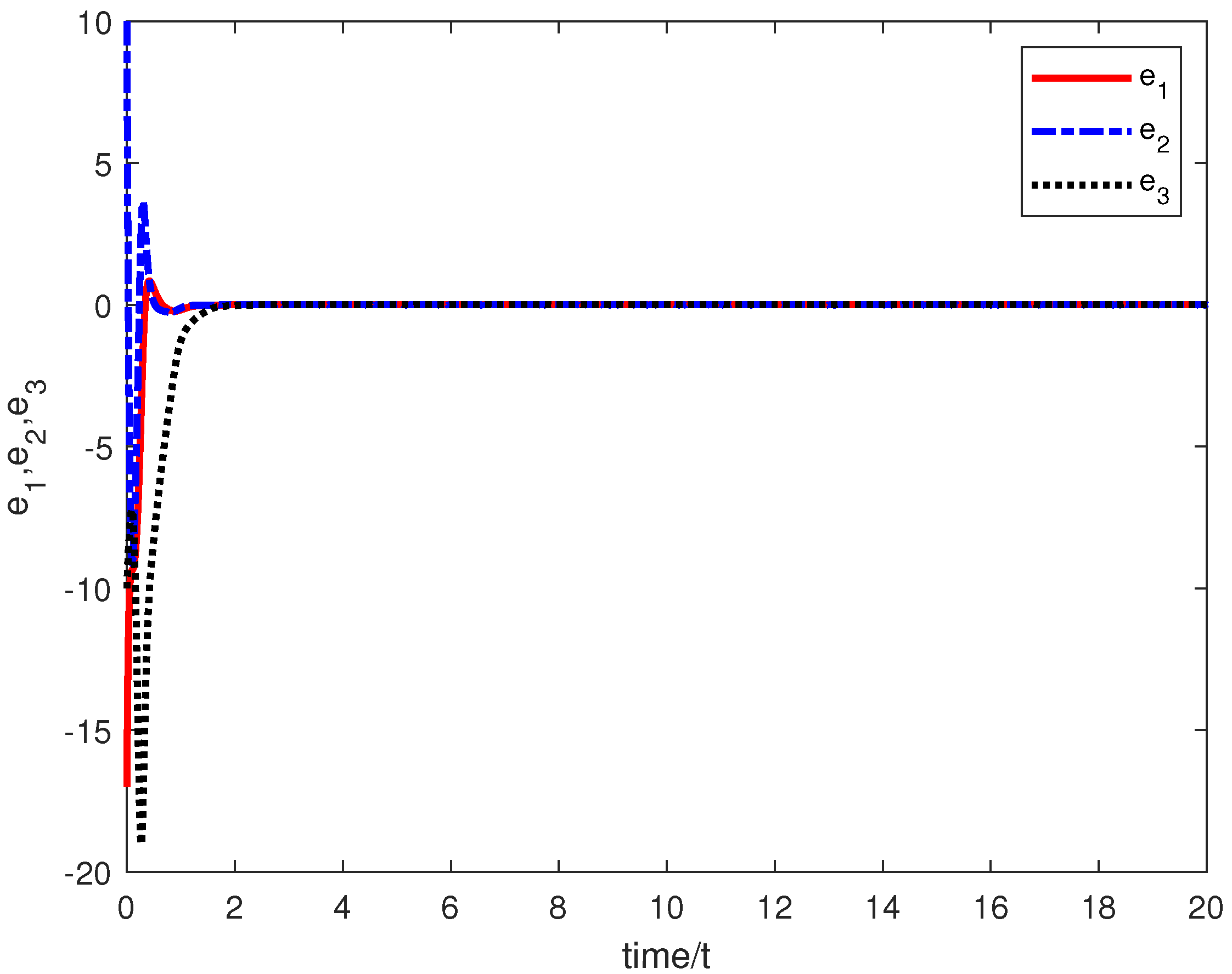
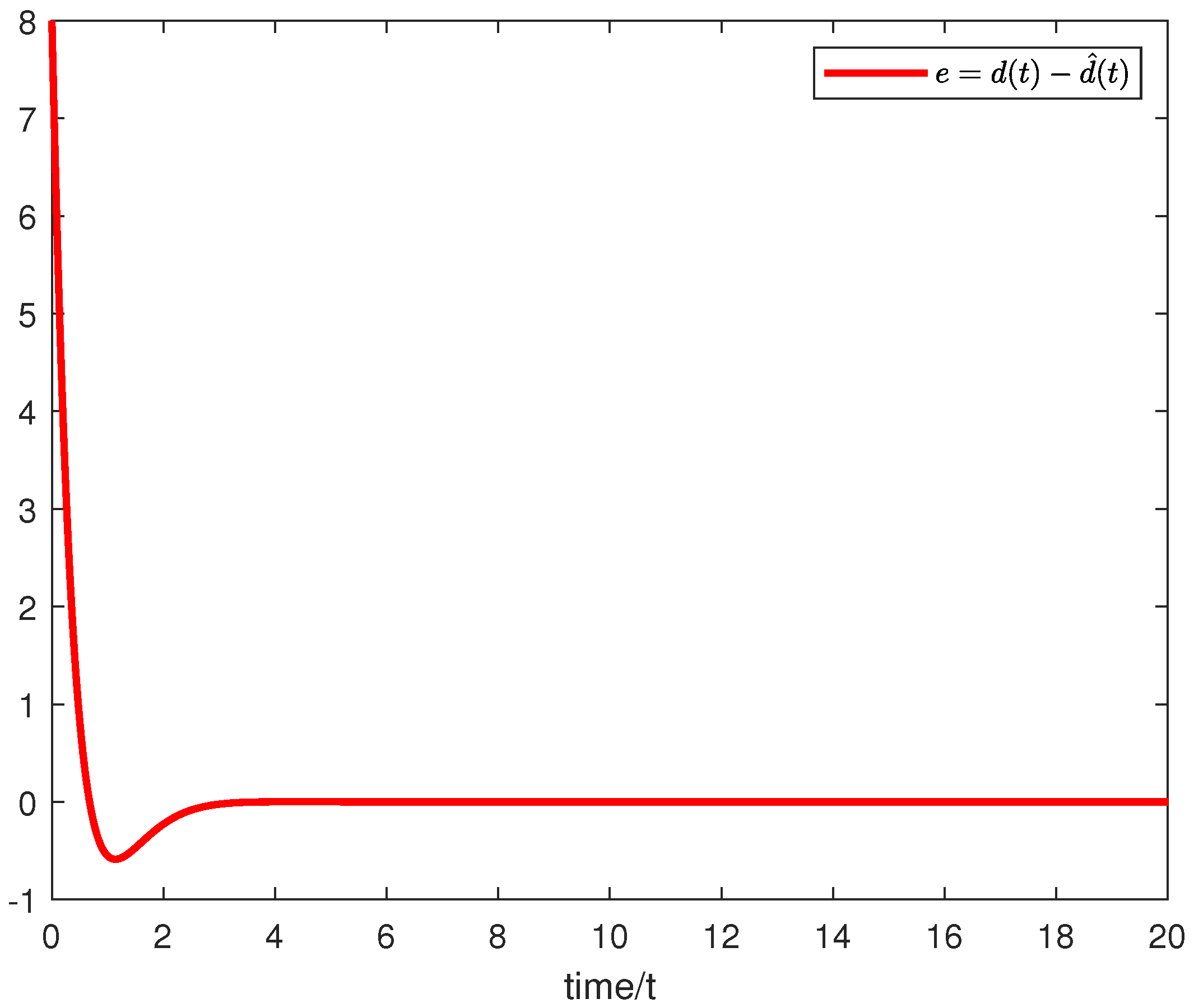
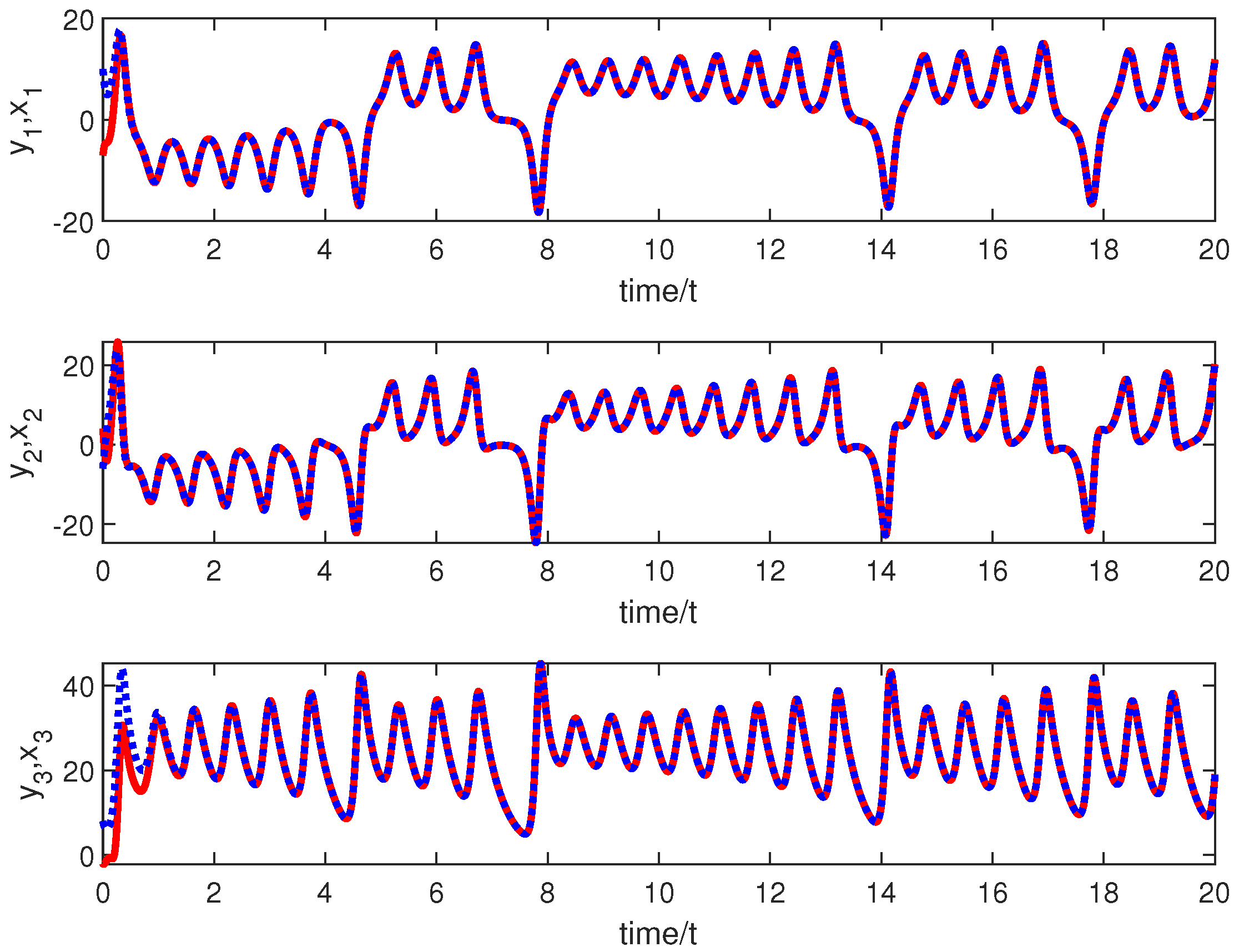
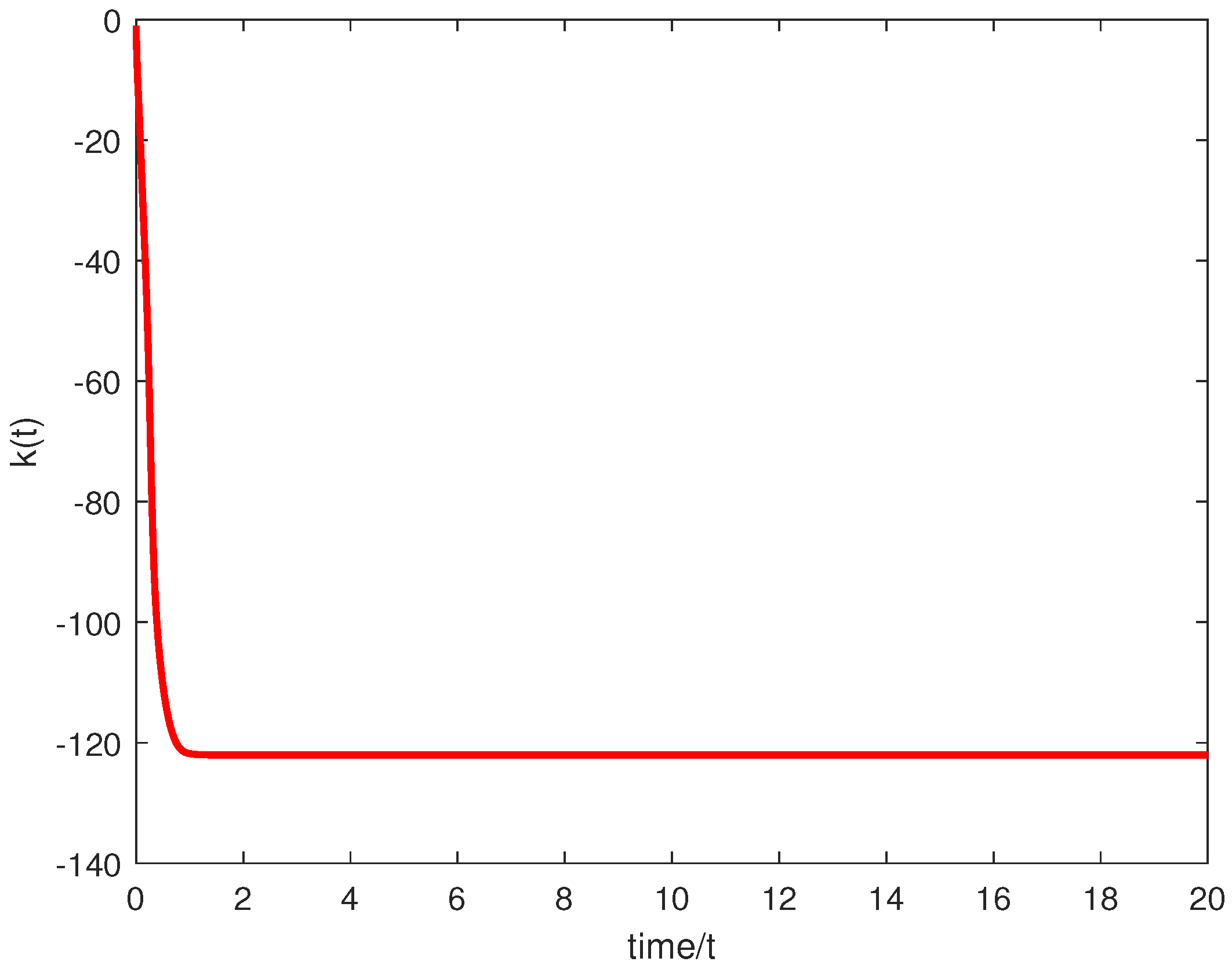
The results of the numerical simulations are presented in Figure 1, Figure 2, Figure 3, Figure 4, Figure 5 and Figure 6 to validate the proposed control scheme. Figure 1 verifies the asymptotic stability of the error system dynamics at the origin, while Figure 2 illustrates the synchronized behavior, wherein the master system states (41) asymptotically approach those of the slave system (44). 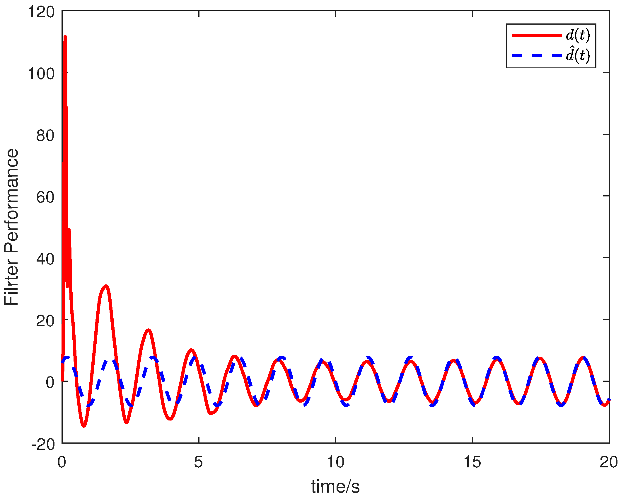The convergence of the dynamic feedback gain $k\left(t\right)$ to a steady-state value is depicted in Figure 3. 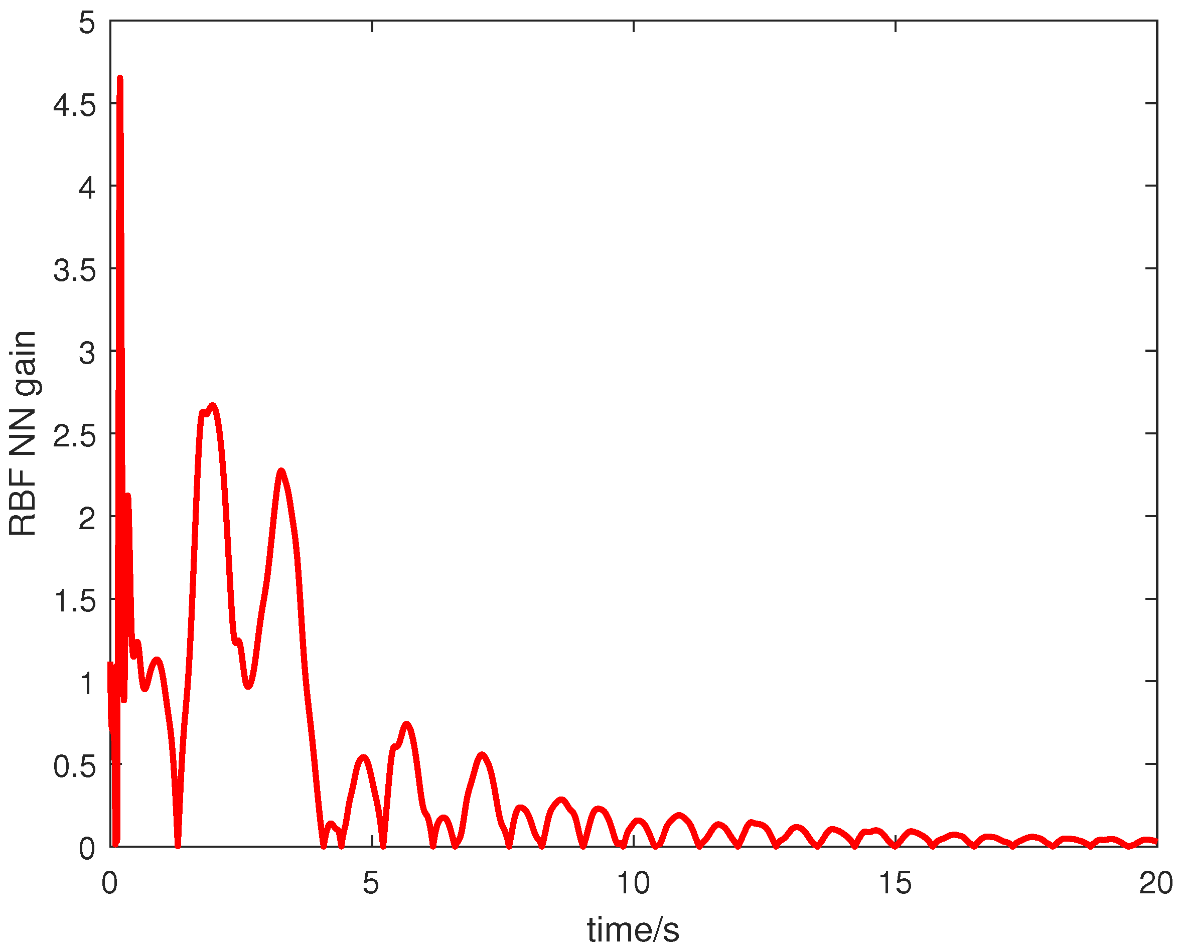The performance of the disturbance estimation mechanism is visualized in Figure 4 and Figure 5; Figure 4 shows the asymptotic tracking of the disturbance $d\left(t\right)$ by its estimate $\widehat{d}\left(t\right)$ and Figure 5 confirms that the corresponding estimation error $e=d\left(t\right)-\widehat{d}\left(t\right)$ converges to zero. Lastly, the output of the RBF-based compensator $u_{\mathrm{rbf}}$ is provided in Figure 6.

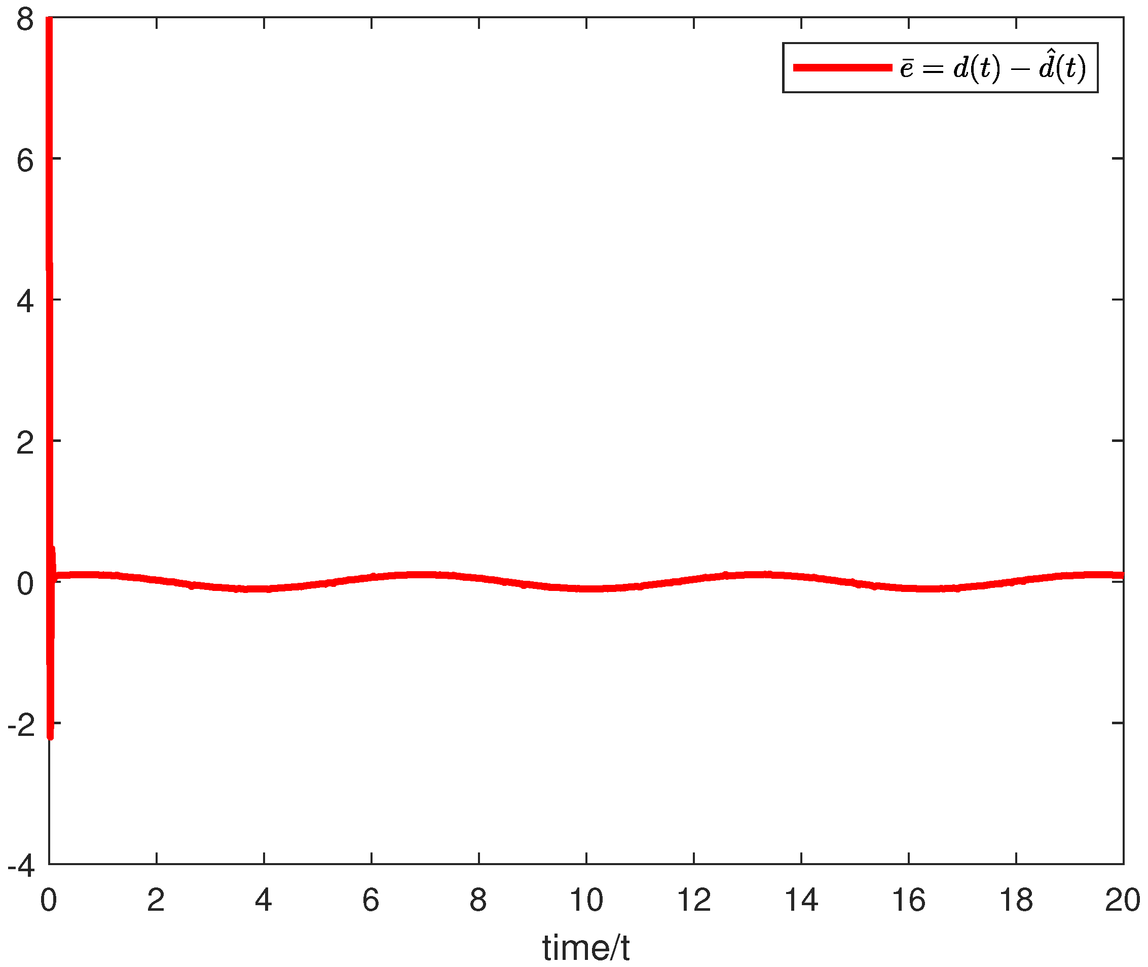
Remark 2.

For the external disturbance $d\left(t\right)=6sin\left(t\right)+8cos\left(t\right)$ considered above, Figure 5 demonstrates that the filter proposed in Equation (48) achieves asymptotic estimation. In contrast, the filter adopted in Ref. [21] is given by

$$G_f\left(s\right)={\displaystyle \frac{a_{1}s+(a_2-w^2)}{s^2+a_{1}s+a_2}}$$

(51)

with $w=4\pi$, $a_1=10w$, and $a_2=100w^2$.

To facilitate a fair comparison, numerical simulations are performed under the same initial conditions as those used in Figure 5. The resulting estimation error $\overline{e}=d\left(t\right)-\widehat{d}\left(t\right)$ is presented in Figure 7. As observed, filter (51) yields only a bounded estimation error, indicating that the associated UDE-based control method achieves robust, rather than asymptotic, disturbance rejection. In other words, the control objective realized by the filter in Ref. [21] is robust in stability, whereas asymptotic disturbance rejection is attained by the proposed filter.

6. Conclusions

This paper investigates the complete synchronization problem for chaotic systems subject to external disturbances and parameter uncertainties and proposes a robust control framework integrating RBF neural networks with disturbance estimation techniques. A dynamic feedback controller is first designed to stabilize the nominal system, followed by a filter-based disturbance estimator for asymptotic disturbance rejection and an RBF neural network compensator to address unmodeled uncertainties. The integrated composite scheme ensures complete synchronization of master–slave chaotic systems under simultaneous disturbances and uncertainties, as validated by numerical simulations on the Lorenz system.

This work focuses on continuous-time chaotic systems; future extensions may include discrete-time and multi-agent chaotic systems, along with structural optimization of the RBF network and disturbance estimator to reduce computational complexity.