A Novel Unit Exponential Delay Time Distribution: Theory, Inference and Applications

Abstract

This paper introduces the Unit Exponential Delay Time Distribution (UEDTD), a two-parameter model for data with support in the unit interval $(0,1)$. The model is derived using two distinct approaches: transformation method applied to the Exponential Delay Time Distribution (EDTD), which itself arises as the convolution of two independent exponential random variables, and product convolution method of two independent power-function random variables that connects UEDTD to Pareto distribution, offering additional interpretability and giving rise to several exact and efficient algorithms for generating random samples. The limit distribution is examined with derivation of key statistical properties. The order statistics with interesting asymptotic results for extremes distribution are discussed and formulated. A reparameterization for the model is suggested to improve estimation stability and formulation with maximum likelihood approach employed for parameter inference. A simulation study demonstrates the consistency and efficiency of the estimators across various sample sizes and parameter configurations. The practical applicability of the UEDTD is demonstrated through a real-world dataset, where it shows superior performance compared to established unit distributions, confirming the utility of the UEDTD for modeling proportional data in applied research.

1. Introduction

Statistical lifetime distributions serve as the foundational framework for analyzing time-to-event data in reliability engineering, survival analysis, and failure-time modeling. Among these, the Exponential Delay Time Distribution (EDTD) emerges naturally from delay-time analysis, a framework for modeling the period between an initial defect and eventual failure (Christer [1] and Christer and Wailer [2,3]). Attia [4] considered the case where both the time of defect occurrence and the delay time are exponentially distributed with different rates ${\lambda }_1$ and ${\lambda }_2$, respectively, where an exponential distribution with rate $\lambda$ is defined by its cumulative distribution function $F\left(x\right)=1-e^{-\lambda x}$ for $x\ge 0$ and has mean $1/\lambda$. The convolution of these two independent exponentials yields the EDTD with probability density function (PDF)

$$f\left(x\right)={\displaystyle \frac{{\lambda }_1{\lambda }_2}{{\lambda }_2-{\lambda }_1}}\left(e^{-{\lambda }_{1}x}-e^{-{\lambda }_{2}x}\right),x>0,{\lambda }_2,{\lambda }_1>0$$

(1)

and corresponding cumulative distribution function (CDF)

$$F\left(x\right)=1-{\displaystyle \frac{1}{{\lambda }_2-{\lambda }_1}}\left({\lambda }_2{e}^{-{\lambda }_{1}x}-{\lambda }_1{e}^{-{\lambda }_{2}x}\right),$$

(2)

The same distribution arises as the sum of two independent exponential random variables (Oguntunde et al. [5]), and it converges to a $\mathrm{Gamma}(2,\lambda )$ distribution when ${\lambda }_1\to {\lambda }_2=\lambda$.

In many scientific fields, including biology, economics, health sciences, and engineering, data often appear as proportions, percentages, or rates restricted to the interval $(0,1)$. Traditional models such as the Beta and Kumaraswamy distributions are commonly employed, but they may lack the flexibility needed to capture complex patterns in modern datasets Mazucheli [6], Sarhan [7]. This limitation has inspired growing interest in unit distributions, which are specifically designed for bounded supports and often derived by transforming existing lifetime distributions via schemes such as the inverse-exponential transformation $Y=e^{-X}$. Recent contributions include the unit Gamma/Gompertz Bantan [8], unit Weibull Mazucheli [6] and Mazucheli [9], unit Burr-XII Korkmaz [10], unit-modified Burr-III Haq [11], unit-Chen Sarhan [12], log-weighted exponential Altun [13], log-Xgamma distribution Altun [14], and unit Rayleigh Bantan [15] distributions, among others.

Given the EDTD’s clear interpretation as the sum of two independent exponential waiting times—a natural representation for processes involving sequential stages, such as defect arrival and failure delay in reliability systems—its transformation to the unit interval promises a valuable new tool for modeling bounded reliability and fractional data. This paper fills that gap by introducing the Unit Exponential Delay Time Distribution (UEDTD), which inherits this structural clarity while offering several distinctive advantages. The UEDTD admits a dual stochastic representation: it can be derived via the transformation $Y=e^{-X}$ where $X\sim \mathrm{EDTD}({\lambda }_1,{\lambda }_2)$, or equivalently as the product of two independent power-function (Beta $({\lambda }_i,1)$) random variables. This product representation offers complementary interpretations in terms of multiplicative effects, while Corollary 1 further connects it to Pareto distributions, linking the model to heavy-tailed phenomena. The UEDTD possesses closed-form expressions for its PDF, CDF, moments, and moment generating function, and its hazard function accommodates increasing and U-shaped patterns. The parameters ${\lambda }_1$ and ${\lambda }_2$ can be interpreted as exponential rates, power-function shape parameters, or Pareto tail indices depending on the representation, enhancing model transparency across different application domains. When ${\lambda }_1,{\lambda }_2\to \lambda$, the UEDTD converges to the well-established UnitGamma $(2,\lambda )$ distribution, ensuring consistency with the EDTD’s gamma limit. Moreover, as derived in Section 4, its extreme value behavior yields asymptotic Weibull and Rayleigh distributions—results not available for most competing models. These features position the UEDTD as a versatile and interpretable alternative to existing unit distributions, with particular appeal in fields where proportional data arise from underlying additive or multiplicative processes.

The structure of the paper proceeds as follows. Section 2 formally introduces the Unit Exponential Delay Time Distribution (UEDTD), detailing its two methods of derivation and provides multiple representations with efficient algorithms for generating random samples. In addition, The limiting distribution is examined along with the validity as a statistical model, demonstrating that when ${\lambda }_1,{\lambda }_2\to \lambda$, the UEDTD converges to a unit Gamma distribution with shape parameter 2, hence preserving the consistency observed in the original EDTD’s Gamma limit and provide an important connection to an established distribution. In Section 3, we derive the essential statistical properties, including moments, the moment-generating function, the hazard function, the quantile function and the mode, along with studying the limit case for the properties confirming the appropriateness to the $\mathrm{UnitGamma}(2,\lambda )$ distribution. Section 4 investigates order statistics and extreme-value theory, proving that the sample minimum converges to a Weibull distribution and the maximum gap from the upper bound converges to a Rayleigh distribution under suitable normalizations. In Section 7, we discuss both point and interval estimation of the UEDTD parameters, reparameterize the model for better stability and formulation. A Monte Carlo simulation study will also be carried out to evaluate the performance of the estimators across different parameter configurations and sample sizes. In Section 6, a real-life dataset is analyzed to demonstrate the practical applicability of the proposed distribution. Section 7 concludes the paper with a summary of key findings and suggestions for future research directions.

2. The Unit Exponential Delay Time Distribution

Recall the Exponential Delay Time Distribution from Section 1 with PDF and CDF given by Equations (1) and (2).We define the Unit Exponential Delay Time Distribution (UEDTD) on the unit interval $(0,1)$ that can be derived through two distinct methodological approaches: transformation method and product convolution method that further connects UEDTD with Pareto distribution. This dual derivation provides deeper insight into the distribution’s structural properties.

2.1. Transformation Method

Let $X\sim \mathrm{EDTD}({\lambda }_1,{\lambda }_2)$ and define the transformation $Y=e^{-X}$. Since X takes values in $(0,\infty )$, the transformed variable Y is constrained to the unit interval $(0,1)$. The cumulative distribution function of Y is obtained through:

$$F_Y\left(y\right)=P(Y\le y)=P(e^{-X}\le y)=P(X\ge -lny)=1-F_X(-lny),0<y<1.$$

Substituting the EDTD CDF from Equation (2) with $x=-lny$ yields:

$$\begin{array}{cc}\hfill F_Y\left(y\right)& =1-\left[1-{\displaystyle \frac{{\lambda }_2{e}^{-{\lambda }_1(-lny)}-{\lambda }_1{e}^{-{\lambda }_2(-lny)}}{{\lambda }_2-{\lambda }_1}}\right]\hfill \\ \hfill & =1-\left[1-{\displaystyle \frac{{\lambda }_2{e}^{{\lambda }_{1}lny}-{\lambda }_1{e}^{{\lambda }_{2}lny}}{{\lambda }_2-{\lambda }_1}}\right]={\displaystyle \frac{{\lambda }_2{y}^{{\lambda }_1}-{\lambda }_1{y}^{{\lambda }_2}}{{\lambda }_2-{\lambda }_1}}.\hfill \end{array}$$

(3)

Differentiating with respect to y gives the probability density function:

$$f_Y\left(y\right)={\displaystyle \frac{{\lambda }_1{\lambda }_2}{{\lambda }_2-{\lambda }_1}}\left(y^{{\lambda }_1-1}-y^{{\lambda }_2-1}\right),0<y<1.$$

(4)

The support is verified through the boundary conditions: $F_Y\left(0\right)=0$ and $F_Y\left(1\right)=1$. Thus, the Equations (3) and (4) define the Unit Exponential Delay Time Distribution (UEDTD) with Y constrained to the unit interval $(0,1)$.

2.2. Convolution Method

An alternative derivation will present the UEDTD as the distribution of the product of two independent power-function random variables.

Lemma 1.

Let $X_i\sim \mathit{Exp}\left({\lambda }_i\right)$, $i=1,2$, be independent exponential random variables. Define $U_i=e^{-X_i}$, which follows the power-function distribution ($\mathit{Beta}({\lambda }_i,1)$) with PDF:

$$f_{U_i}\left(u\right)={\lambda }_i{u}^{{\lambda }_i-1},0<u<1.$$

Then the product $Y=U_1{U}_2$ follows $\mathit{UEDTD}({\lambda }_1,{\lambda }_2)$.

Proof. 

The transformation $U_i=e^{-X_i}$ where $X_i\sim \mathrm{Exp}\left({\lambda }_i\right)$ yields:

$$f_{U_i}\left(u\right)=f_{X_i}(-lnu)·\left|{\displaystyle \frac{d}{du}}(-lnu)\right|={\lambda }_i{e}^{-{\lambda }_i(-lnu)}·{\displaystyle \frac{1}{u}}={\lambda }_i{u}^{{\lambda }_i-1}.$$

For the product $Y=U_1{U}_2$, let $V=U_1$ so that $Y=V{U}_2$ and $U_2=Y/V$. The Jacobian of this transformation is $\left|J\right|=1/\left|v\right|$. The joint density of $(V,Y)$ is:

$$f_{V,Y}(v,y)=f_{U_1}\left(v\right)f_{U_2}(y/v)·{\displaystyle \frac{1}{v}}.$$

Marginalizing over v gives:

$$\begin{array}{cc}\hfill f_Y\left(y\right)& ={\int }_{v=y}^1{f}_{U_1}\left(v\right)f_{U_2}(y/v)·{\displaystyle \frac{1}{v}}dv={\int }_{v=y}^1{\lambda }_1{v}^{{\lambda }_1-1}·{\lambda }_2{(y/v)}^{{\lambda }_2-1}·{\displaystyle \frac{1}{v}}dv={\lambda }_1{\lambda }_2{y}^{{\lambda }_2-1}{\int }_{v=y}^1{v}^{{\lambda }_1-{\lambda }_2-1}dv.\hfill \end{array}$$

Evaluating the integral for ${\lambda }_1\ne {\lambda }_2$:

$${\int }_{v=y}^1{v}^{{\lambda }_1-{\lambda }_2-1}dv={\left[{\displaystyle \frac{v^{{\lambda }_1-{\lambda }_2}}{{\lambda }_1-{\lambda }_2}}\right]}_{v=y}^1={\displaystyle \frac{1-y^{{\lambda }_1-{\lambda }_2}}{{\lambda }_1-{\lambda }_2}}.$$

Thus:

$$f_Y\left(y\right)={\lambda }_1{\lambda }_2{y}^{{\lambda }_2-1}·{\displaystyle \frac{1-y^{{\lambda }_1-{\lambda }_2}}{{\lambda }_1-{\lambda }_2}}={\displaystyle \frac{{\lambda }_1{\lambda }_2}{{\lambda }_1-{\lambda }_2}}\left(y^{{\lambda }_2-1}-y^{{\lambda }_1-1}\right)={\displaystyle \frac{{\lambda }_1{\lambda }_2}{{\lambda }_2-{\lambda }_1}}\left(y^{{\lambda }_1-1}-y^{{\lambda }_2-1}\right),$$

which matches Equation (4). □

Corollary 1 (Pareto Product Representation). 

Let $X_1$ and $X_2$ be independent random variables with Pareto distributions $F_{X_i}\left(x\right)=1-x^{-{\lambda }_i}$ for $x\ge 1$, $i=1,2$. Then $Y={\left(X_1{X}_2\right)}^{-1}$ follows a $\mathrm{UEDTD}({\lambda }_1,{\lambda }_2)$ distribution.

Proof. 

For each i, consider the transformation $U_i=X_i^{-1}$. For $0<u<1$,

$$F_{U_i}\left(u\right)=P(X_i^{-1}\le u)=P(X_i\ge u^{-1})=u^{{\lambda }_i},$$

so that $f_{U_i}\left(u\right)={\lambda }_i{u}^{{\lambda }_i-1}$, which is precisely the power-function distribution from Lemma 1. Since $Y=U_1{U}_2$, the result follows directly from Lemma 1. □

Proposition 1 (Power Transformation). 

If $Y\sim \mathrm{UEDTD}({\lambda }_1,{\lambda }_2)$ with ${\lambda }_1,{\lambda }_2>0$ and $p>0$, then $Y^p\sim \mathrm{UEDTD}({\lambda }_1/p,{\lambda }_2/p)$.

Proof. 

For $0<y<1$, the cumulative distribution function of $Y^p$ is:

$$F_{Y^p}\left(y\right)=P(Y^p\le y)=P(Y\le y^{1/p})=F_Y\left(y^{1/p}\right),$$

where $F_Y$ is the UEDTD CDF given in (3). Substituting,

$$F_{Y^p}\left(y\right)={\displaystyle \frac{{\lambda }_2{\left(y^{1/p}\right)}^{{\lambda }_1}-{\lambda }_1{\left(y^{1/p}\right)}^{{\lambda }_2}}{{\lambda }_2-{\lambda }_1}}={\displaystyle \frac{{\lambda }_2{y}^{{\lambda }_1/p}-{\lambda }_1{y}^{{\lambda }_2/p}}{{\lambda }_2-{\lambda }_1}}.$$

Differentiating with respect to y yields the density:

$$f_{Y^p}\left(y\right)={\displaystyle \frac{({\lambda }_1/p)({\lambda }_2/p)}{({\lambda }_2/p)-({\lambda }_1/p)}}\left(y^{({\lambda }_1/p)-1}-y^{({\lambda }_2/p)-1}\right),$$

which is precisely the UEDTD density in (4) with parameters ${\lambda }_1/p$ and ${\lambda }_2/p$. □

Remark 1.

The multiple representations of the UEDTD offer complementary theoretical and practical insights. The transformation method links the distribution to EDTD and exponential waiting-time structures, particularly useful in reliability modeling. The product construction provides a multiplicative interpretation relevant to fields such as economics and biology, while Corollary 1 connects UEDTD to heavy-tailed Pareto distributions. Together, these constructions enrich parameter interpretability (${\lambda }_i$ as rates, shape parameters, or tail indices) and suggest various algorithms for random sample generation, as detailed in the following subsection.

2.3. Random Variate Generation

The previous multiple representations naturally give rise to several exact and efficient algorithms for generating random samples from the UEDTD. We present two primary methods below (Algorithm 1 and Algorithm 2); both avoid rejection sampling and are straightforward to implement. Alternatively, as noted in Corollary 1, one can generate two independent Pareto random variables $X_1\sim \mathrm{Pareto}\left({\lambda }_1\right)$, $X_2\sim \mathrm{Pareto}\left({\lambda }_2\right)$, then set $Y=1/\left(X_1{X}_2\right)$, which is equivalent to Algorithm 1 after transformation.

Algorithm 1 Product of Power-Function Random Variables (Recommended)

This follows directly from Lemma 1 and the inverse transform sampling for the power-function distribution. 1. Generate two independent uniform random variables $U_1,U_2\sim \mathrm{Uniform}(0,1)$. 2. Compute $Y=U_1^{1/{\lambda }_1}\times U_2^{1/{\lambda }_2}$. 3. Return $Y\sim \mathrm{UEDTD}({\lambda }_1,{\lambda }_2)$. (Note: $U^{1/\lambda }$ is the inverse CDF of the power-function/Beta($\lambda$,1) distribution.)

Algorithm 2 Exponential Sum + Transformation

This follows from the transformation method in Section 2.1. 1. Generate two independent exponential random variables: $X_1\sim \mathrm{Exp}\left({\lambda }_1\right)$, $X_2\sim \mathrm{Exp}\left({\lambda }_2\right)$. 2. Compute $X=(X_1+X_2)\sim EDTD({\lambda }_1,{\lambda }_2)$. 3. Set $Y=e^{-X}$. 4. Return $Y\sim \mathrm{UEDTD}({\lambda }_1,{\lambda }_2)$.

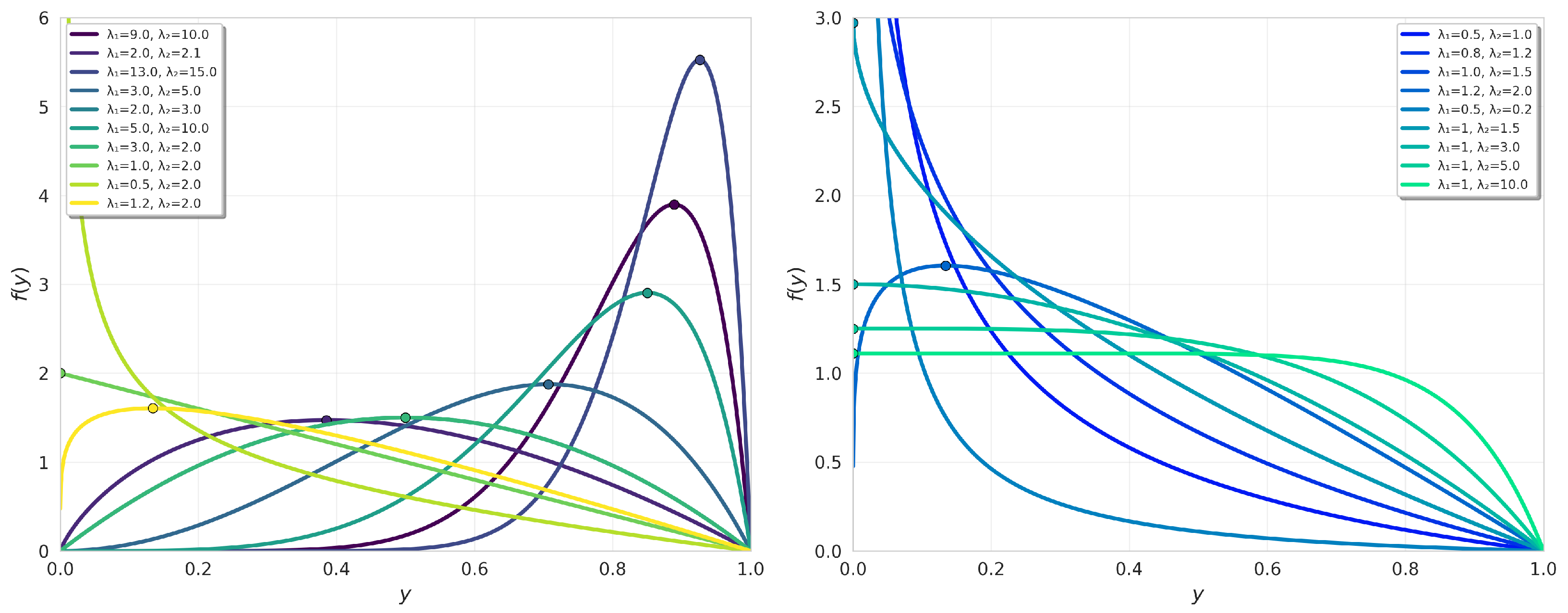
These algorithms are exact (no approximation or rejection), fast, and leverage standard uniform/exponential generators available in most statistical software (R, Python, MATLAB, etc.). In simulation studies (Section 6), we use Algorithm 1 to generate Monte Carlo samples due to its simplicity and direct link to the power-function representation. Figure 1 showes the PDF of the UEDTD for various parameter combinations.

The validity of the UEDTD as a distribution function can be verified via normalization as follows:

$$\begin{array}{cc}\hfill {\int }_0^1{f}_Y\left(y\right)dy& ={\displaystyle \frac{{\lambda }_1{\lambda }_2}{{\lambda }_2-{\lambda }_1}}{\int }_0^1\left(y^{{\lambda }_1-1}-y^{{\lambda }_2-1}\right)dy={\displaystyle \frac{{\lambda }_1{\lambda }_2}{{\lambda }_2-{\lambda }_1}}{\left[{\displaystyle \frac{y^{{\lambda }_1}}{{\lambda }_1}}-{\displaystyle \frac{y^{{\lambda }_2}}{{\lambda }_2}}\right]}_0^1={\displaystyle \frac{{\lambda }_1{\lambda }_2}{{\lambda }_2-{\lambda }_1}}·{\displaystyle \frac{{\lambda }_2-{\lambda }_1}{{\lambda }_1{\lambda }_2}}=1.\hfill \end{array}$$

For non-negativity: since $y^{{\lambda }_1-1}>y^{{\lambda }_2-1}$ for $0<y<1$ when ${\lambda }_2>{\lambda }_1>0$,$y^{{\lambda }_2-1}>y^{{\lambda }_1-1}$ for $0<y<1$ when ${\lambda }_1>{\lambda }_2>0$ and the coefficient ${\displaystyle \frac{{\lambda }_1{\lambda }_2}{{\lambda }_2-{\lambda }_1}}>0$, we have $f_Y\left(y\right)>0$ on $(0,1)$. Thus, UEDTD is a valid probability distribution.

2.4. Limiting Distribution of the UEDTD

As the parameters ${\lambda }_1$ and ${\lambda }_2$ converge, we will show that the UEDTD approaches the Unit Gamma distribution, an established distribution for bounded data (Ratnaparkhi and Mosimann [16]; Grassia [17]) with probability density function, cumulative distribution function, moment generating function, mean, and variance are given, respectively, by:

$$\begin{array}{cc}\hfill f_{\mathrm{UG}(\alpha ,\lambda )}\left(y\right)& ={\displaystyle \frac{{\lambda }^{\alpha }}{\mathsf{\Gamma }\left(\alpha \right)}}{y}^{\lambda -1}{(-lny)}^{\alpha -1},0<y<1,\hfill \end{array}$$

(5)

$$\begin{array}{cc}\hfill F_{\mathrm{UG}(\alpha ,\lambda )}\left(y\right)& =1-{\displaystyle \frac{\gamma (\alpha ,-\lambda lny)}{\mathsf{\Gamma }\left(\alpha \right)}},0<y<1,\hfill \end{array}$$

(6)

$$\begin{array}{cc}\hfill M_{\mathrm{UG}(\alpha ,\lambda )}\left(t\right)& =\sum _{k=0}^{\infty }{\displaystyle \frac{t^k}{k!}}{\left({\displaystyle \frac{\lambda }{k+\lambda }}\right)}^{\alpha },t\in \mathbb{R},\hfill \end{array}$$

(7)

$$\begin{array}{cc}\hfill E_{\mathrm{UG}(\alpha ,\lambda )}\left[Y\right]& ={\left(1+{\displaystyle \frac{1}{\lambda }}\right)}^{-\alpha },\hfill \end{array}$$

(8)

$$\begin{array}{cc}\hfill {\mathrm{Var}}_{\mathrm{UG}(\alpha ,\lambda )}\left(Y\right)& ={\left(1+{\displaystyle \frac{2}{\lambda }}\right)}^{-\alpha }-{\left(1+{\displaystyle \frac{1}{\lambda }}\right)}^{-2\alpha },\hfill \end{array}$$

(9)

where $\gamma (·,·)$ denotes the lower incomplete gamma function.

This connection to an established distribution demonstrates consistency and provides important insights.

Lemma 2.

Let $Y\sim \mathrm{UEDTD}({\lambda }_1,{\lambda }_2)$ with ${\lambda }_1,{\lambda }_2>0$. As ${\lambda }_1,{\lambda }_2\to \lambda$, Y converges in distribution to a unit Gamma distribution with shape parameter 2 and rate parameter λ denoted by $\mathrm{UnitGamma}(2,\lambda )$.

Proof. 

From the density of the UEDTD given in (4), we have:

$$f_Y\left(y\right)={\displaystyle \frac{{\lambda }_1{\lambda }_2}{{\lambda }_2-{\lambda }_1}}\left(y^{{\lambda }_1-1}-y^{{\lambda }_2-1}\right)={\lambda }_1{\lambda }_2{y}^{{\lambda }_1-1}\left({\displaystyle \frac{1-y^{{\lambda }_2-{\lambda }_1}}{{\lambda }_2-{\lambda }_1}}\right),0<y<1.$$

Taking the limit as ${\lambda }_1,{\lambda }_2\to \lambda$ and using the standard limit ${\displaystyle \underset{\epsilon \to 0}{lim}\frac{1-y^{\epsilon }}{\epsilon }=-lny}$, we obtain:

$$\underset{{\lambda }_1,{\lambda }_2\to \lambda }{lim}{f}_Y\left(y\right)={\lambda }^2{y}^{\lambda -1}(-lny),$$

which is the probability density function of $\mathrm{UnitGamma}(2,\lambda )$, confirming pointwise convergence of the densities. By Scheffé’s lemma [18], this implies the stated convergence in distribution. □

The limit of some key statistical properties will also be discussed in the following section.

2.5. Identifiability Considerations and Parameter Ordering

An important consideration for the UEDTD—inherited from the EDTD—is parameter identifiability. The moment generating function of the EDTD is given by

$$M_X\left(t\right)={\displaystyle \frac{{\lambda }_1{\lambda }_2}{({\lambda }_1-t)({\lambda }_2-t)}},$$

whose poles are precisely at $t={\lambda }_1$ and $t={\lambda }_2$. If two distinct parameter pairs $({\lambda }_1,{\lambda }_2)$ and $({\lambda }_1^{\prime },{\lambda }_2^{\prime })$ yield the same distribution, their MGFs must coincide, forcing the pole sets $\{{\lambda }_1,{\lambda }_2\}$ and $\{{\lambda }_1^{\prime },{\lambda }_2^{\prime }\}$ to be identical. Consequently, the parameters are uniquely determined except for their order, the distributions corresponding to $({\lambda }_1,{\lambda }_2)$ and $({\lambda }_2,{\lambda }_1)$ are the same. This slight ambiguity is removed by imposing an ordering constraint, conventionally ${\lambda }_2>{\lambda }_1>0,$ which we adopt throughout this paper.

The same identifiability structure carries over to the UEDTD via the transformation $Y=e^{-X}$. Since the mapping $X\mapsto Y$ is one-to-one, the UEDTD inherits the identifiability-up-to-permutation property and its PDF satisfies

$$f_Y(y;{\lambda }_1,{\lambda }_2)=f_Y(y;{\lambda }_2,{\lambda }_1),y\in (0,1).$$

Under the constraint ${\lambda }_2>{\lambda }_1$, several distributional characteristics become ordered interpretably:

• The exponent ${\lambda }_1$ governs the lower-tail behavior: smaller ${\lambda }_1$ yields heavier density near $y=0$.
• The difference ${\lambda }_2-{\lambda }_1$ controls the separation between the two exponential components, influencing modality and skewness.

If the alternative ordering ${\lambda }_1>{\lambda }_2>0$ were used, all distributional properties would remain mathematically valid, but the roles of ${\lambda }_1$ and ${\lambda }_2$ in expressions for tail behavior, moments, and hazard shapes would be exchanged. The adopted ordering ${\lambda }_2>{\lambda }_1$ provides a consistent framework for interpretation, estimation, and inference. In the degenerate case ${\lambda }_1={\lambda }_2=\lambda$, the distribution reduces to the fully identifiable $\mathrm{UnitGamma}(2,\lambda )$ model.

3. Statistical Properties and Limiting Case

In this section, we derive the key distributional properties of the UEDTD along with some limiting and asymptotic behaviors.

3.1. Moments and Moment Generating Function

The moments of the UEDTD provide essential insight into its central tendency and shape. For $Y\sim \mathrm{UEDTD}({\lambda }_1,{\lambda }_2)$, the r-th raw moment can be derived directly as follows

$$\begin{array}{cc}\hfill \mathbb{E}\left[Y^r\right]& ={\int }_0^1{y}^r{f}_Y\left(y\right)dy={\displaystyle \frac{{\lambda }_1{\lambda }_2}{{\lambda }_2-{\lambda }_1}}{\int }_0^1\left(y^{r+{\lambda }_1-1}-y^{r+{\lambda }_2-1}\right)dy\hfill \\ \hfill & ={\displaystyle \frac{{\lambda }_1{\lambda }_2}{{\lambda }_2-{\lambda }_1}}\left[{\displaystyle \frac{1}{r+{\lambda }_1}}-{\displaystyle \frac{1}{r+{\lambda }_2}}\right]={\displaystyle \frac{{\lambda }_1{\lambda }_2}{(r+{\lambda }_1)(r+{\lambda }_2)}},\hfill \end{array}$$

(10)

which exists for all $r>-min({\lambda }_1,{\lambda }_2)$.

From the general moment Formula (10), the mean is obtained by setting $r=1$:

$$\mu ={\displaystyle \frac{{\lambda }_1{\lambda }_2}{({\lambda }_1+1)({\lambda }_2+1)}}.$$

(11)

The second raw moment, ${\mu }_2^{\prime }={\lambda }_1{\lambda }_2/\left[({\lambda }_1+2)({\lambda }_2+2)\right]$, yields the variance after subtracting ${\mu }^2$ as follows

$$\mathrm{Var}\left(Y\right)=\mathbb{E}\left[Y^2\right]-{\left(\mathbb{E}\left[Y\right]\right)}^2={\displaystyle \frac{{\lambda }_1{\lambda }_2}{({\lambda }_1+2)({\lambda }_2+2)}}-{\left[{\displaystyle \frac{{\lambda }_1{\lambda }_2}{({\lambda }_1+1)({\lambda }_2+1)}}\right]}^2.$$

(12)

Algebraic simplification gives more explicit form

$${\sigma }^2={\displaystyle \frac{{\lambda }_1{\lambda }_2\left[{({\lambda }_1+1)}^2{({\lambda }_2+1)}^2-{\lambda }_1{\lambda }_2({\lambda }_1+2)({\lambda }_2+2)\right]}{{({\lambda }_1+1)}^2{({\lambda }_2+1)}^2({\lambda }_1+2)({\lambda }_2+2)}}.$$

(13)

Higher-order central moments ${\mu }_n=\mathbb{E}\left[{(Y-\mu )}^n\right]$ can be expressed as:

$${\mu }_n=\sum _{k=0}^n\left({\displaystyle \genfrac{}{}{0pt}{}{n}{k}}\right){(-\mu )}^{n-k}{\mu }_k^{\prime },$$

(14)

where ${\mu }_k^{\prime }={\displaystyle \frac{{\lambda }_1{\lambda }_2}{(k+{\lambda }_1)(k+{\lambda }_2)}}$.

• Skewness and kurtosis. The skewness and kurtosis of the UEDTD can be expressed compactly in terms of the raw moments and the variance as follows: The skewness coefficient is:

$${\gamma }_1={\displaystyle \frac{{\mu }_3}{{\sigma }^3}}={\displaystyle \frac{\mathbb{E}\left[{(Y-\mu )}^3\right]}{{\sigma }^3}}={\displaystyle \frac{{\mu }_3^{\prime }-3\mu {\mu }_2^{\prime }+2{\mu }^3}{{\sigma }^3}},$$

(15)

and the excess kurtosis is:

$${\gamma }_2={\displaystyle \frac{{\mu }_4}{{\sigma }^4}}-3={\displaystyle \frac{\mathbb{E}\left[{(Y-\mu )}^4\right]}{{\sigma }^4}}-3={\displaystyle \frac{{\mu }_4^{\prime }-4\mu {\mu }_3^{\prime }+6{\mu }^2{\mu }_2^{\prime }-3{\mu }^4}{{\sigma }^2}}-3.$$

(16)

These can be expanded explicitly as:

$$\begin{array}{cc}\hfill {\gamma }_1& ={\displaystyle \frac{\frac{{\lambda }_1{\lambda }_2}{({\lambda }_1+3)({\lambda }_2+3)}-3\mu \frac{{\lambda }_1{\lambda }_2}{({\lambda }_1+2)({\lambda }_2+2)}+2{\mu }^3}{{\left[\frac{{\lambda }_1{\lambda }_2}{({\lambda }_1+2)({\lambda }_2+2)}-{\mu }^2\right]}^{3/2}}},\hfill \\ \hfill {\gamma }_2& ={\displaystyle \frac{\frac{{\lambda }_1{\lambda }_2}{({\lambda }_1+4)({\lambda }_2+4)}-4\mu \frac{{\lambda }_1{\lambda }_2}{({\lambda }_1+3)({\lambda }_2+3)}+6{\mu }^2\frac{{\lambda }_1{\lambda }_2}{({\lambda }_1+2)({\lambda }_2+2)}-3{\mu }^4}{{\left[\frac{{\lambda }_1{\lambda }_2}{({\lambda }_1+2)({\lambda }_2+2)}-{\mu }^2\right]}^2}}-3,\hfill \end{array}$$

(17)

where $\mu ={\displaystyle \frac{{\lambda }_1{\lambda }_2}{({\lambda }_1+1)({\lambda }_2+1)}}$.

While fully expanded expressions are algebraically complex, these forms are computationally efficient and reveal the symmetric dependence on ${\lambda }_1$ and ${\lambda }_2$.

The skewness and kurtosis coefficients characterize the shape of the UEDTD. For fixed ${\lambda }_2$, skewness decreases as ${\lambda }_1$ increases, with the distribution becoming less asymmetric for larger parameter values. Positive skewness is most pronounced when ${\lambda }_1$ is small, indicating concentration of probability mass near zero. The excess kurtosis is positive for all finite parameter combinations, confirming that the UEDTD is leptokurtic (heavier tails than the normal distribution). In the limiting case ${\lambda }_1={\lambda }_2=\lambda$, both skewness and kurtosis approach zero as $\lambda \to \infty$, consistent with the convergence to a symmetric light-tailed distribution.

Lemma 3 (Moment Generating Function). 

Let $Y\sim \mathit{UEDTD}({\lambda }_1,{\lambda }_2)$. The moment generating function $M_Y\left(t\right)=\mathbb{E}\left[e^{tY}\right]$ is given by:

$$M_Y\left(t\right)={\displaystyle \frac{{\lambda }_1{\lambda }_2}{{\lambda }_2-{\lambda }_1}}\left[{\displaystyle \frac{1}{{\lambda }_1}}{}_{1}F_1({\lambda }_1;{\lambda }_1+1;t)-{\displaystyle \frac{1}{{\lambda }_2}}{}_{1}F_1({\lambda }_2;{\lambda }_2+1;t)\right],$$

where ${}_{1}F_1(a;b;z)$ denotes Kummer’s confluent hypergeometric function. Equivalently, in series form:

$$M_Y\left(t\right)={\lambda }_1{\lambda }_2\sum _{k=0}^{\infty }{\displaystyle \frac{t^k}{k!(k+{\lambda }_1)(k+{\lambda }_2)}}.$$

Proof. 

Starting from the definition:

$$M_Y\left(t\right)={\int }_0^1{e}^{ty}{f}_Y\left(y\right)dy={\displaystyle \frac{{\lambda }_1{\lambda }_2}{{\lambda }_2-{\lambda }_1}}{\int }_0^1{e}^{ty}\left(y^{{\lambda }_1-1}-y^{{\lambda }_2-1}\right)dy.$$

Consider the integral $I(a,t)={\int }_0^1{e}^{ty}{y}^{a-1}dy$. Expanding $e^{ty}$ as a power series:

$$I(a,t)={\int }_0^1\sum _{k=0}^{\infty }{\displaystyle \frac{t^k{y}^k}{k!}}{y}^{a-1}dy=\sum _{k=0}^{\infty }{\displaystyle \frac{t^k}{k!}}{\int }_0^1{y}^{k+a-1}dy=\sum _{k=0}^{\infty }{\displaystyle \frac{t^k}{k!(k+a)}}.$$

This sum is recognized as a representation of the confluent hypergeometric function:

$$I(a,t)={\displaystyle \frac{1}{a}}{}_{1}F_1(a;a+1;t),$$

since by definition,

$${}_{1}F_1(a;a+1;t)=\sum _{k=0}^{\infty }{\displaystyle \frac{{\left(a\right)}_k}{{(a+1)}_k}}{\displaystyle \frac{t^k}{k!}}=a\sum _{k=0}^{\infty }{\displaystyle \frac{t^k}{k!(k+a)}},$$

where ${\left(a\right)}_k=a(a+1)\cdots (a+k-1)$ is the Pochhammer symbol.

Applying this to the MGF:

$$\begin{array}{cc}\hfill M_Y\left(t\right)& ={\displaystyle \frac{{\lambda }_1{\lambda }_2}{{\lambda }_2-{\lambda }_1}}\left[I({\lambda }_1,t)-I({\lambda }_2,t)\right]={\displaystyle \frac{{\lambda }_1{\lambda }_2}{{\lambda }_2-{\lambda }_1}}\left[{\displaystyle \frac{1}{{\lambda }_1}}{}_{1}F_1({\lambda }_1;{\lambda }_1+1;t)-{\displaystyle \frac{1}{{\lambda }_2}}{}_{1}F_1({\lambda }_2;{\lambda }_2+1;t)\right].\hfill \end{array}$$

(18)

The series form follows directly from the series expansion of $I(a,t)$:

$$M_Y\left(t\right)={\displaystyle \frac{{\lambda }_1{\lambda }_2}{{\lambda }_2-{\lambda }_1}}\sum _{k=0}^{\infty }{\displaystyle \frac{t^k}{k!}}\left({\displaystyle \frac{1}{k+{\lambda }_1}}-{\displaystyle \frac{1}{k+{\lambda }_2}}\right)={\lambda }_1{\lambda }_2\sum _{k=0}^{\infty }{\displaystyle \frac{t^k}{k!(k+{\lambda }_1)(k+{\lambda }_2)}}.$$

(19)

The series representation provides a practical computational method, while the ${}_{1}F_1$ form connects UEDTD to the well-studied class of confluent hypergeometric functions. This connection facilitates analytical manipulations and asymptotic analysis of the distribution.

The characteristic function ${\varphi }_Y\left(t\right)=\mathbb{E}\left[e^{itY}\right]$ can be obtained by replacing t with $it$ in $M_Y\left(t\right)$. □

3.2. Hazard Function

The hazard (failure rate) function for UEDTD can be obtained from its PDF and survival function as follows:

$$h_Y\left(y\right)={\displaystyle \frac{f_Y\left(y\right)}{S_Y\left(y\right)}}={\displaystyle \frac{{\lambda }_1{\lambda }_2\left(y^{{\lambda }_1-1}-y^{{\lambda }_2-1}\right)}{{\lambda }_2(1-y^{{\lambda }_1})-{\lambda }_1(1-y^{{\lambda }_2})}},0<y<1,$$

(20)

where $S_Y\left(y\right)=1-F_Y\left(y\right)={\displaystyle \frac{{\lambda }_2(1-y^{{\lambda }_1})-{\lambda }_1(1-y^{{\lambda }_2})}{{\lambda }_2-{\lambda }_1}}$ denotes the survival function.

Studying the asymptotic behavior of the hazard function at the interval boundaries provides critical insights into failure mechanisms.

As $y\to 0^{+}$, the leading term approximation yields:

$$h_Y\left(y\right)\sim {\displaystyle \frac{{\lambda }_1{\lambda }_2}{{\lambda }_2-{\lambda }_1}}{y}^{{\lambda }_1-1}.$$

This approximation leads to three distinct regimes for the initial hazard:

$$\underset{y\to 0^{+}}{lim}{h}_Y\left(y\right)=\left\{\begin{array}{cc}\infty \hfill & \mathrm{if}{\lambda }_1<1,\hfill \\ {\displaystyle \frac{{\lambda }_1{\lambda }_2}{{\lambda }_1+{\lambda }_2}}\hfill & \mathrm{if}{\lambda }_1=1,\hfill \\ 0\hfill & \mathrm{if}{\lambda }_1>1.\hfill \end{array}\right.$$

Thus ${\lambda }_1$ alone determines the initial hazard: unbounded for ${\lambda }_1<1$, finite for ${\lambda }_1=1$, and vanishing for ${\lambda }_1>1$.

As $y\to 1^{-}$, using the approximation $y^{\lambda }\approx 1+\lambda lny$ yields:

$$\underset{y\to 1^{-}}{lim}{h}_Y\left(y\right)={\displaystyle \frac{{\lambda }_1{\lambda }_2}{{\lambda }_1+{\lambda }_2}}.$$

(21)

Unlike the initial hazard, the terminal hazard depends symmetrically on both parameters, representing a balanced combination of the two rate parameters.

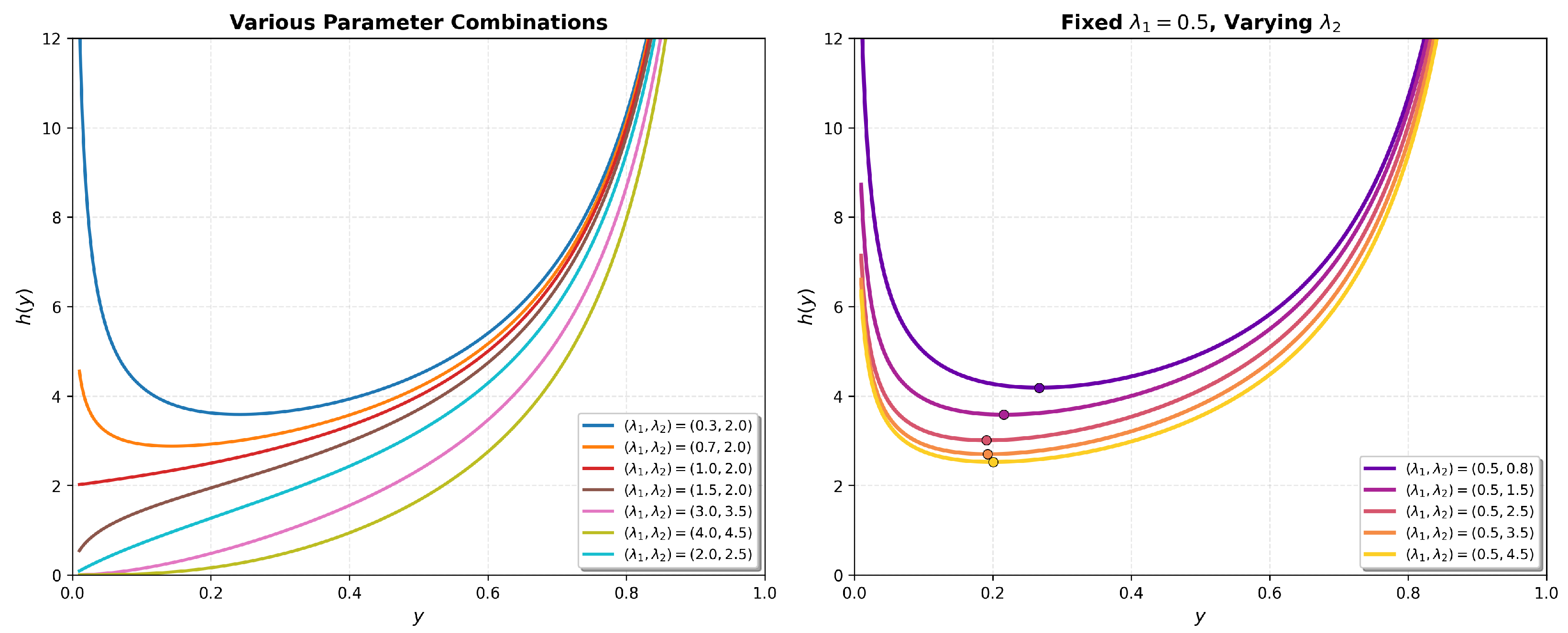
Under the constraint ${\lambda }_2>{\lambda }_1>0$, the UEDTD hazard function exhibits two characteristic shapes, as illustrated in Figure 2:

• Increasing Hazard Rate (IFR): When ${\lambda }_1>1$ (which implies ${\lambda }_2>{\lambda }_1>1$), the hazard function increases monotonically from $h\left(0^{+}\right)=0$ to the finite terminal value $h\left(1^{-}\right)={\lambda }_1{\lambda }_2/({\lambda }_1+{\lambda }_2)$. This pattern characterizes systems subject to wear-out failures, where the failure rate increases with time or usage.
• U-Shaped Hazard: When ${\lambda }_1<1$, the hazard function exhibits a U-shaped pattern: decreasing from $h\left(0^{+}\right)=\infty$ to a minimum, then increasing toward the finite terminal value $h\left(1^{-}\right)={\lambda }_1{\lambda }_2/({\lambda }_1+{\lambda }_2)$. This pattern models systems experiencing high initial failure rates (infant mortality), followed by a period of increasing failure rates due to aging or wear-out, though without an extended constant hazard region.

The flexibility of the hazard function to model both increasing and U-shaped failure rates makes UEDTD particularly suitable for reliability analysis where failure mechanisms may evolve over time, encompassing both early-life failures and aging effects within the bounded domain $(0,1)$.

3.3. Mode and Quantiles

The mode of the UEDTD distribution, when it exists, is the value $y_{\mathrm{mode}}\in (0,1)$ that maximizes the probability density function $f_Y\left(y\right)$. Differentiating $f_Y\left(y\right)$ in (4) and setting it equal to zero yields the mode as follows:

$$({\lambda }_1-1)y^{{\lambda }_1-2}=({\lambda }_2-1)y^{{\lambda }_2-2}.$$

Rearranging terms:

$$({\lambda }_1-1)y^{{\lambda }_1-{\lambda }_2}={\lambda }_2-1,$$

Thus,

$$y_{\mathrm{mode}}={\left({\displaystyle \frac{{\lambda }_2-1}{{\lambda }_1-1}}\right)}^{1/({\lambda }_1-{\lambda }_2)},$$

(22)

provided that ${\lambda }_1>1$ or ${\lambda }_2>1$, and ${\lambda }_1\ne 1$, ${\lambda }_2\ne 1$.

The p-th quantile $y_p=F_Y^{-1}\left(p\right)$ of the UEDTD is shown to satisfy the nonlinear equation:

$${\lambda }_2{y}_p^{{\lambda }_1}-{\lambda }_1{y}_p^{{\lambda }_2}=p({\lambda }_2-{\lambda }_1).$$

(23)

By definition, $F_Y\left(y_p\right)=p$. Substituting the CDF using (3):

$${\displaystyle \frac{{\lambda }_2{y}_p^{{\lambda }_1}-{\lambda }_1{y}_p^{{\lambda }_2}}{{\lambda }_2-{\lambda }_1}}=p.$$

Multiplying both sides by $({\lambda }_2-{\lambda }_1)$ yields the stated result.

3.4. Limiting Distributional Properties

Lemma 4.

Let $Y\sim \mathrm{UEDTD}({\lambda }_1,{\lambda }_2)$ with ${\lambda }_1,{\lambda }_2>0$. As ${\lambda }_1,{\lambda }_2\to \lambda >0$:

(i) 

The cumulative distribution function of Y converges pointwise to that of $\mathrm{UnitGamma}(2,\lambda )$;

(ii) 

The hazard function of Y converges pointwise to that of $\mathrm{UnitGamma}(2,\lambda )$;

(iii) 

The mean and variance of Y converge to those of $\mathrm{UnitGamma}(2,\lambda )$;

(iv) 

The moment generating function of Y converges pointwise to that of $\mathrm{UnitGamma}(2,\lambda )$.

Proof. 

We verify each property separately.

(i) 

Cumulative Distribution Function: From the CDF of Y given in (3), we have:

$$F_Y\left(y\right)={\displaystyle \frac{{\lambda }_2{y}^{{\lambda }_1}-{\lambda }_1{y}^{{\lambda }_2}}{{\lambda }_2-{\lambda }_1}}=y^{{\lambda }_1}+{\lambda }_1{y}^{{\lambda }_1}\left({\displaystyle \frac{1-y^{{\lambda }_2-{\lambda }_1}}{{\lambda }_2-{\lambda }_1}}\right),0<y<1.$$

Taking the limit and using the standard limit ${\displaystyle \underset{\epsilon \to 0}{lim}\frac{1-y^{\epsilon }}{\epsilon }=-lny}$, we obtain for each $y\in (0,1)$:

$$\underset{{\lambda }_1,{\lambda }_2\to \lambda }{lim}{F}_Y\left(y\right)=y^{\lambda }+\lambda y^{\lambda }(-lny)=y^{\lambda }\left(1-\lambda lny\right),$$

which is precisely $F_{\mathrm{UG}(2,\lambda )}\left(y\right)$. Hence, pointwise convergence of the CDF is established.

(ii) 

Hazard Function: The hazard function of Y is defined as $h_Y\left(y\right)=f_Y\left(y\right)/(1-F_Y\left(y\right))$. From Lemma 2 and part (i) above, we have for each $y\in (0,1)$:

$$\underset{{\lambda }_1,{\lambda }_2\to \lambda }{lim}{h}_{Y({\lambda }_1,{\lambda }_2)}\left(y\right)={\displaystyle \frac{{\displaystyle \underset{{\lambda }_1,{\lambda }_2\to \lambda }{lim}{f}_{Y({\lambda }_1,{\lambda }_2)}\left(y\right)}}{{\displaystyle \underset{{\lambda }_1,{\lambda }_2\to \lambda }{lim}(1-F_{Y({\lambda }_1,{\lambda }_2)}\left(y\right))}}}={\displaystyle \frac{{\lambda }^2{y}^{\lambda -1}(-lny)}{1-y^{\lambda }(1-\lambda lny)}},$$

which matches $h_{\mathrm{UG}(2,\lambda )}\left(y\right)$. This establishes pointwise convergence of the hazard function.

(iii) 

Mean and Variance: The mean of Y is given by (11). Taking the limit as ${\lambda }_1,{\lambda }_2\to \lambda$:

$$\underset{{\lambda }_1,{\lambda }_2\to \lambda }{lim}{\mu }_{Y({\lambda }_1,{\lambda }_2)}={\displaystyle \frac{{\lambda }^2}{{(\lambda +1)}^2}}={\left(1+{\displaystyle \frac{1}{\lambda }}\right)}^{-2}={\mu }_{\mathrm{UG}(2,\lambda )}.$$

Similarly, from the variance expression (8):

$$\underset{{\lambda }_1,{\lambda }_2\to \lambda }{lim}{\sigma }_{Y({\lambda }_1,{\lambda }_2)}^2={\displaystyle \frac{{\lambda }^2}{{(\lambda +2)}^2}}-{\displaystyle \frac{{\lambda }^4}{{(\lambda +1)}^4}}={\left(1+{\displaystyle \frac{2}{\lambda }}\right)}^{-2}-{\left(1+{\displaystyle \frac{1}{\lambda }}\right)}^{-4}={\sigma }_{\mathrm{UG}(2,\lambda )}^2.$$

Thus, the mean and variance converge to those of $\mathrm{UnitGamma}(2,\lambda )$.

(iv) 

Moment Generating Function: From Lemma 3, the moment generating function of Y is:

$$M_Y\left(t\right)={\lambda }_1{\lambda }_2\sum _{k=0}^{\infty }{\displaystyle \frac{t^k}{k!(k+{\lambda }_1)(k+{\lambda }_2)}},t\in \mathbb{R}.$$

Taking the limit as ${\lambda }_1,{\lambda }_2\to \lambda$

$$\underset{{\lambda }_1,{\lambda }_2\to \lambda }{lim}{\lambda }_1{\lambda }_2\sum _{k=0}^{\infty }{\displaystyle \frac{t^k}{k!(k+{\lambda }_1)(k+{\lambda }_2)}}.$$

In order to interchange the limit and summation, we apply the Dominated Convergence Theorem.

For ${\lambda }_1,{\lambda }_2$ sufficiently close to $\lambda$, there exist constants $0<m\le M$ such that $m\le {\lambda }_1,{\lambda }_2\le M$ (e.g., take $m=\lambda /2$ and $M=3\lambda /2$). Then for all $k\ge 0$:

$$\left|{\displaystyle \frac{{\lambda }_1{\lambda }_2}{(k+{\lambda }_1)(k+{\lambda }_2)}}\right|\le {\displaystyle \frac{M^2}{{(k+m)}^2}}\le {\displaystyle \frac{C}{k^2+1}}$$

for some constant C (e.g., $C=M^2·max(1/m^2,2)$). Consequently,

$$\left|{\lambda }_1{\lambda }_2{\displaystyle \frac{t^k}{k!(k+{\lambda }_1)(k+{\lambda }_2)}}\right|\le {\displaystyle \frac{C}{k^2+1}}·{\displaystyle \frac{{\left|t\right|}^k}{k!}}.$$

The series ${\displaystyle \sum _{k=0}^{\infty }\frac{C}{k^2+1}·\frac{{\left|t\right|}^k}{k!}}$ converges, since

$$\sum _{k=0}^{\infty }{\displaystyle \frac{C}{k^2+1}}·{\displaystyle \frac{{\left|t\right|}^k}{k!}}\le C\sum _{k=0}^{\infty }{\displaystyle \frac{{\left|t\right|}^k}{k!}}=C{e}^{\left|t\right|}<\infty .$$

Thus, by the Dominated Convergence Theorem, we may interchange the limit and the sum, yields:

$$\underset{{\lambda }_1,{\lambda }_2\to \lambda }{lim}{M}_Y\left(t\right)=\sum _{k=0}^{\infty }{\displaystyle \frac{t^k}{k!}}{\left({\displaystyle \frac{\lambda }{k+\lambda }}\right)}^2,$$

which is precisely the moment generating function of $\mathrm{UnitGamma}(2,\lambda )$, thus establishing pointwise convergence of the moment generating function. □

4. Order Statistics

This section examines the order statistics of the Unit Exponential Delay Time Distribution (UEDTD), which are essential for analyzing extreme values and ranges in bounded data. The distribution of order statistics provides fundamental insights into the behavior of sample minima, maxima, and intermediate order statistics. Additionally, we derive the limiting distributions of the sample minimum and maximum, establishing convergence to well-known extreme value distributions.

4.1. Distribution of Order Statistics

Let $Y_1,Y_2,\dots ,Y_n$ constitute a random sample from $\mathrm{UEDTD}({\lambda }_1,{\lambda }_2)$, and denote by $Y_{\left(1\right)}\le Y_{\left(2\right)}\le \cdots \le Y_{\left(n\right)}$ the corresponding order statistics. The probability density function of the k-th order statistic $Y_{\left(k\right)}$ is given by the general formula:

$$f_{Y_{\left(k\right)}}\left(y\right)={\displaystyle \frac{n!}{(k-1)!(n-k)!}}{\left[F_Y\left(y\right)\right]}^{k-1}{[1-F_Y\left(y\right)]}^{n-k}{f}_Y\left(y\right),0<y<1,$$

where $F_Y\left(y\right)$ and $f_Y\left(y\right)$ are the cumulative distribution function and probability density function of UEDTD given by Equations (3) and (4), respectively. Substituting the specific forms yields:

$$\begin{array}{cc}\hfill f_{Y_{\left(k\right)}}\left(y\right)& ={\displaystyle \frac{n!}{(k-1)!(n-k)!}}{\left[{\displaystyle \frac{{\lambda }_2{y}^{{\lambda }_1}-{\lambda }_1{y}^{{\lambda }_2}}{{\lambda }_2-{\lambda }_1}}\right]}^{k-1}{\left[1-{\displaystyle \frac{{\lambda }_2{y}^{{\lambda }_1}-{\lambda }_1{y}^{{\lambda }_2}}{{\lambda }_2-{\lambda }_1}}\right]}^{n-k}\left[{\displaystyle \frac{{\lambda }_1{\lambda }_2}{{\lambda }_2-{\lambda }_1}}\left(y^{{\lambda }_1-1}-y^{{\lambda }_2-1}\right)\right].\hfill \end{array}$$

(24)

Of particular interest are the extreme order statistics. The probability density function of the sample minimum $Y_{\left(1\right)}$ simplifies to:

$$\begin{array}{cc}\hfill f_{Y_{\left(1\right)}}\left(y\right)& =n{[1-F_Y\left(y\right)]}^{n-1}{f}_Y\left(y\right)=n{\left[{\displaystyle \frac{{\lambda }_2(1-y^{{\lambda }_1})-{\lambda }_1(1-y^{{\lambda }_2})}{{\lambda }_2-{\lambda }_1}}\right]}^{n-1}\left[{\displaystyle \frac{{\lambda }_1{\lambda }_2}{{\lambda }_2-{\lambda }_1}}\left(y^{{\lambda }_1-1}-y^{{\lambda }_2-1}\right)\right].\hfill \end{array}$$

(25)

Similarly, the density of the sample maximum $Y_{\left(n\right)}$ is:

$$\begin{array}{cc}\hfill f_{Y_{\left(n\right)}}\left(y\right)& =n{\left[F_Y\left(y\right)\right]}^{n-1}{f}_Y\left(y\right)=n{\left[{\displaystyle \frac{{\lambda }_2{y}^{{\lambda }_1}-{\lambda }_1{y}^{{\lambda }_2}}{{\lambda }_2-{\lambda }_1}}\right]}^{n-1}\left[{\displaystyle \frac{{\lambda }_1{\lambda }_2}{{\lambda }_2-{\lambda }_1}}\left(y^{{\lambda }_1-1}-y^{{\lambda }_2-1}\right)\right].\hfill \end{array}$$

(26)

The sample range $R=Y_{\left(n\right)}-Y_{\left(1\right)}$, measuring the spread between extreme values, follows the distribution:

$$F_R\left(r\right)=n{\int }_0^{1-r}{[F_Y(y+r)-F_Y\left(y\right)]}^{n-1}{f}_Y\left(y\right)dy,0<r<1,$$

(27)

where

$$F_Y(y+r)-F_Y\left(y\right)={\displaystyle \frac{{\lambda }_2{(y+r)}^{{\lambda }_1}-{\lambda }_1{(y+r)}^{{\lambda }_2}-{\lambda }_2{y}^{{\lambda }_1}+{\lambda }_1{y}^{{\lambda }_2}}{{\lambda }_2-{\lambda }_1}}.$$

4.2. Limiting Distribution of the Minimum

Theorem 1.

Let $Y_1,Y_2,\dots ,Y_n$ be i.i.d. $\mathrm{UEDTD}({\lambda }_1,{\lambda }_2)$ random variables with ${\lambda }_2>{\lambda }_1>0$, and let $Y_{\left(1\right)}=min\{Y_1,\dots ,Y_n\}$ be the sample minimum. Define the normalized minimum $Z_n=n^{1/{\lambda }_1}{Y}_{\left(1\right)}$.

Then, as $n\to \infty$, the normalized minimum $Z_n$ converges in distribution to a Weibull distribution with shape parameter ${\lambda }_1$ and scale parameter $\sigma ={\left({\displaystyle \frac{{\lambda }_2}{{\lambda }_2-{\lambda }_1}}\right)}^{1/{\lambda }_1}$. That is,

$$\underset{n\to \infty }{lim}\mathbb{P}(Z_n>t)=exp\left(-{\displaystyle \frac{{\lambda }_2}{{\lambda }_2-{\lambda }_1}}{t}^{{\lambda }_1}\right),t>0.$$

Proof. 

We first establish an asymptotic approximation for $F_Y\left(y\right)$ as $y\to 0^{+}$. From the cumulative distribution function (3):

$$F_Y\left(y\right)={\displaystyle \frac{{\lambda }_2{y}^{{\lambda }_1}-{\lambda }_1{y}^{{\lambda }_2}}{{\lambda }_2-{\lambda }_1}}.$$

Since ${\lambda }_2>{\lambda }_1>0$, for $y\to 0^{+}$ we have $y^{{\lambda }_2}=o\left(y^{{\lambda }_1}\right)$ as ${\lambda }_2$ is higher order than ${\lambda }_1$. Consequently,

$$F_Y\left(y\right)={\displaystyle \frac{{\lambda }_2}{{\lambda }_2-{\lambda }_1}}{y}^{{\lambda }_1}-{\displaystyle \frac{{\lambda }_1}{{\lambda }_2-{\lambda }_1}}{y}^{{\lambda }_2}={\displaystyle \frac{{\lambda }_2}{{\lambda }_2-{\lambda }_1}}{y}^{{\lambda }_1}+o\left(y^{{\lambda }_1}\right).$$

Thus, the asymptotic approximation is:

$$F_Y\left(y\right)\sim {\displaystyle \frac{{\lambda }_2}{{\lambda }_2-{\lambda }_1}}{y}^{{\lambda }_1}\mathrm{as}y\to 0^{+}.$$

(28)

Now consider the survival function of the normalized minimum:

$$\begin{array}{cc}\hfill \mathbb{P}(Z_n>t)& =\mathbb{P}\left(n^{1/{\lambda }_1}{Y}_{\left(1\right)}>t\right)=\mathbb{P}\left(Y_{\left(1\right)}>{\displaystyle \frac{t}{n^{1/{\lambda }_1}}}\right)={\left[1-F_Y\left({\displaystyle \frac{t}{n^{1/{\lambda }_1}}}\right)\right]}^n.\hfill \end{array}$$

Applying the asymptotic approximation (28) with $y=t/n^{1/{\lambda }_1}$:

$$F_Y\left({\displaystyle \frac{t}{n^{1/{\lambda }_1}}}\right)\sim {\displaystyle \frac{{\lambda }_2}{{\lambda }_2-{\lambda }_1}}{\left({\displaystyle \frac{t}{n^{1/{\lambda }_1}}}\right)}^{{\lambda }_1}={\displaystyle \frac{{\lambda }_2}{{\lambda }_2-{\lambda }_1}}·{\displaystyle \frac{t^{{\lambda }_1}}{n}}.$$

Therefore,

$$1-F_Y\left({\displaystyle \frac{t}{n^{1/{\lambda }_1}}}\right)\sim 1-{\displaystyle \frac{{\lambda }_2}{{\lambda }_2-{\lambda }_1}}·{\displaystyle \frac{t^{{\lambda }_1}}{n}}.$$

Taking the limit as $n\to \infty$:

$$\begin{array}{cc}\hfill \underset{n\to \infty }{lim}\mathbb{P}(Z_n>t)& =\underset{n\to \infty }{lim}{\left[1-{\displaystyle \frac{{\lambda }_2}{{\lambda }_2-{\lambda }_1}}·{\displaystyle \frac{t^{{\lambda }_1}}{n}}\right]}^n=exp\left(-{\displaystyle \frac{{\lambda }_2}{{\lambda }_2-{\lambda }_1}}{t}^{{\lambda }_1}\right).\hfill \end{array}$$

(29)

The expression in (29) is precisely the survival function of a Weibull random variable with shape parameter ${\lambda }_1$ and scale parameter $\sigma ={\left({\displaystyle \frac{{\lambda }_2}{{\lambda }_2-{\lambda }_1}}\right)}^{1/{\lambda }_1}$, completing the proof. □

Remark 2.

The convergence to a Weibull distribution confirms that UEDTD belongs to the Type III (Weibull) domain of attraction for minima, characteristic of distributions bounded below at zero (Gnedenko [19], Beirlant [20]). In extreme value theory, the shape parameter of the limiting Weibull distribution is determined only by the exponent ${\lambda }_1$ in the lower tail expansion $F_Y\left(y\right)\sim c{y}^{{\lambda }_1}$ de Haan [21]. The scale parameter incorporates both ${\lambda }_1$ and ${\lambda }_2$ through the ratio ${\displaystyle \frac{{\lambda }_2}{{\lambda }_2-{\lambda }_1}}$, reflecting their joint influence on the concentration of probability mass near the lower bound. This result aligns with recent developments in extreme value analysis for bounded distributions (Gomes [22]) and finds applications in reliability engineering and risk assessment Albrecher [23].

4.3. Limiting Distribution of the Maximum

Theorem 2.

Let $Y_1,Y_2,\dots ,Y_n$ be i.i.d. $\mathrm{UEDTD}({\lambda }_1,{\lambda }_2)$ random variables, and let $Y_{\left(n\right)}=max\{Y_1,\dots ,Y_n\}$ denote the sample maximum. Define the normalized gap from the upper bound $W_n=\sqrt{n}(1-Y_{\left(n\right)})$. Then, as $n\to \infty$, $W_n$ converges in distribution to a Rayleigh distribution with scale parameter $\sigma =\sqrt{1/\left({\lambda }_1{\lambda }_2\right)}$. That is,

$$\underset{n\to \infty }{lim}\mathbb{P}(W_n\le t)=1-exp\left(-{\displaystyle \frac{{\lambda }_1{\lambda }_2}{2}}{t}^2\right),t>0.$$

Proof. 

For y near 1, let $u=1-y$. Using the Taylor expansion $y^{\lambda }=e^{\lambda lny}=1-\lambda u+{\displaystyle \frac{\lambda (\lambda -1)}{2}}{u}^2+O\left(u^3\right)$, we obtain:

$$F_Y(1-u)={\displaystyle \frac{{\lambda }_2{(1-u)}^{{\lambda }_1}-{\lambda }_1{(1-u)}^{{\lambda }_2}}{{\lambda }_2-{\lambda }_1}}.$$

Expanding both terms:

$$\begin{array}{cc}\hfill {(1-u)}^{{\lambda }_i}& =1-{\lambda }_{i}u+{\displaystyle \frac{{\lambda }_i({\lambda }_i-1)}{2}}{u}^2+O\left(u^3\right),i=1,2.\hfill \end{array}$$

Substituting these expansions:

$$\begin{array}{cc}\hfill F_Y(1-u)& ={\displaystyle \frac{{\lambda }_2\left[1-{\lambda }_{1}u+\frac{{\lambda }_1({\lambda }_1-1)}{2}{u}^2\right]-{\lambda }_1\left[1-{\lambda }_{2}u+\frac{{\lambda }_2({\lambda }_2-1)}{2}{u}^2\right]}{{\lambda }_2-{\lambda }_1}}+O\left(u^3\right)\hfill \\ \hfill & ={\displaystyle \frac{({\lambda }_2-{\lambda }_1)-{\lambda }_1{\lambda }_{2}u+{\lambda }_1{\lambda }_{2}u+\frac{{\lambda }_1{\lambda }_2({\lambda }_1-1)-{\lambda }_1{\lambda }_2({\lambda }_2-1)}{2}{u}^2}{{\lambda }_2-{\lambda }_1}}+O\left(u^3\right)\hfill \\ \hfill & =1-{\displaystyle \frac{{\lambda }_1{\lambda }_2}{2}}{u}^2+O\left(u^3\right).\hfill \end{array}$$

Thus, the asymptotic approximation is:

$$1-F_Y(1-u)\sim {\displaystyle \frac{{\lambda }_1{\lambda }_2}{2}}{u}^2\mathrm{as}u\to 0^{+}.$$

(30)

Now, consider the cumulative distribution function of $W_n$:

$$\mathbb{P}(W_n\le t)=\mathbb{P}\left(1-Y_{\left(n\right)}\le {\displaystyle \frac{t}{\sqrt{n}}}\right)=1-{\left[F_Y\left(1-{\displaystyle \frac{t}{\sqrt{n}}}\right)\right]}^n.$$

Using the asymptotic expansion (30) with $u=t/\sqrt{n}$:

$$F_Y\left(1-{\displaystyle \frac{t}{\sqrt{n}}}\right)=1-{\displaystyle \frac{{\lambda }_1{\lambda }_2}{2}}·{\displaystyle \frac{t^2}{n}}+O\left(n^{-3/2}\right).$$

Therefore,

$$\underset{n\to \infty }{lim}{\left[F_Y\left(1-{\displaystyle \frac{t}{\sqrt{n}}}\right)\right]}^n=\underset{n\to \infty }{lim}{\left[1-{\displaystyle \frac{{\lambda }_1{\lambda }_2}{2}}·{\displaystyle \frac{t^2}{n}}+O\left(n^{-3/2}\right)\right]}^n=exp\left(-{\displaystyle \frac{{\lambda }_1{\lambda }_2}{2}}{t}^2\right).$$

Hence,

$$\underset{n\to \infty }{lim}\mathbb{P}(W_n\le t)=1-exp\left(-{\displaystyle \frac{{\lambda }_1{\lambda }_2}{2}}{t}^2\right),t>0,$$

(31)

which is the cumulative distribution function of a Rayleigh distribution with scale parameter $\sigma =\sqrt{1/\left({\lambda }_1{\lambda }_2\right)}$. □

Remark 3.

The convergence to a Rayleigh distribution (which is a Weibull distribution with shape parameter 2) indicates that the maximum of UEDTD samples approaches the upper bound at a rate of $1/\sqrt{n}$. This quadratic decay $1-F_Y(1-u)\sim {\displaystyle \frac{{\lambda }_1{\lambda }_2}{2}}{u}^2$ occurs because the probability density function $f_Y\left(y\right)$ approaches zero linearly as $y\to 1^{-}$, specifically $f_Y\left(y\right)\sim {\lambda }_1{\lambda }_2(1-y)$ Arnold [24]. Distributions with finite upper bounds and smooth densities vanishing at the boundary typically exhibit this quadratic tail behavior. The scale parameter $\sigma =\sqrt{1/\left({\lambda }_1{\lambda }_2\right)}$ demonstrates that larger rate parameters result in faster convergence of the maximum to the upper bound, with the maximum more tightly clustered near 1.

5. Estimation and Simulation Study

In this section, we discuss the maximum likelihood estimation approach for both point and interval estimation of the UEDTD parameters. A reparameterization for the model will also be suggested enhancing the derivation, stability and estimation process along with two proposed algorithms for obtaining the MLEs. A comprehensive simulation study will also be conducted to evaluate the performance of the estimators across different parameter configurations and sample sizes.

5.1. Maximum Likelihood Estimation

Let $y_1,y_2,\dots ,y_n$ be an independent and identically distributed sample from $\mathrm{UEDTD}({\lambda }_1,{\lambda }_2)$, with $0<y_i<1$ for $i=1,\dots ,n$. Then, the likelihood function is:

$$L({\lambda }_1,{\lambda }_2;\mathbf{y})=\prod _{i=1}^n{\displaystyle \frac{{\lambda }_1{\lambda }_2}{{\lambda }_2-{\lambda }_1}}\left(y_i^{{\lambda }_1-1}-y_i^{{\lambda }_2-1}\right).$$

(32)

and the log-likelihood function takes the form:

$$\mathcal{l}({\lambda }_1,{\lambda }_2)=nln\left({\lambda }_1\right)+nln\left({\lambda }_2\right)-nln({\lambda }_2-{\lambda }_1)+\sum _{i=1}^{n}ln\left(y_i^{{\lambda }_1-1}-y_i^{{\lambda }_2-1}\right).$$

(33)

In order to provide the ML estimators, we obtain the first derivatives and equate to 0 as follows:

$$\begin{array}{cc}\hfill {\displaystyle \frac{\partial \mathcal{l}}{\partial {\lambda }_1}}& ={\displaystyle \frac{n}{{\lambda }_1}}+{\displaystyle \frac{n}{{\lambda }_2-{\lambda }_1}}+\sum _{i=1}^n{\displaystyle \frac{y_i^{{\lambda }_1-1}ln{y}_i}{y_i^{{\lambda }_1-1}-y_i^{{\lambda }_2-1}}}=0,\hfill \end{array}$$

(34)

$$\begin{array}{cc}\hfill {\displaystyle \frac{\partial \mathcal{l}}{\partial {\lambda }_2}}& ={\displaystyle \frac{n}{{\lambda }_2}}-{\displaystyle \frac{n}{{\lambda }_2-{\lambda }_1}}-\sum _{i=1}^n{\displaystyle \frac{y_i^{{\lambda }_2-1}ln{y}_i}{y_i^{{\lambda }_1-1}-y_i^{{\lambda }_2-1}}}=0.\hfill \end{array}$$

(35)

A reparameterization is suggested to improve the numerical stability and ensure the constraint ${\lambda }_2>{\lambda }_1>0$. Let

$$\alpha ={\lambda }_1,\beta ={\lambda }_2-{\lambda }_1>0,$$

(36)

so that ${\lambda }_1=\alpha$, ${\lambda }_2=\alpha +\beta$.

Lemma 5.

The maximum likelihood estimators $(\widehat{\alpha },\widehat{\beta })$ satisfy:

$$\begin{array}{c}\hfill {\displaystyle \frac{1}{\widehat{\alpha }}}+{\displaystyle \frac{1}{\widehat{\alpha }+\widehat{\beta }}}=-\overline{\mathcal{l}},{\displaystyle \frac{1}{\widehat{\alpha }+\widehat{\beta }}}-{\displaystyle \frac{1}{\widehat{\beta }}}=S_1\left(\widehat{\beta }\right),\end{array}$$

(37)

where $\overline{\mathcal{l}}=n^{-1}{\sum }_{i=1}^{n}ln{y}_i$ and $S_1\left(\beta \right)=n^{-1}{\sum }_{i=1}^n{\displaystyle \frac{y_i^{\beta }ln{y}_i}{1-y_i^{\beta }}}$.

Proof. 

Under the reparameterization (36), the probability density function becomes:

$$f_Y(y;\alpha ,\beta )={\displaystyle \frac{\alpha (\alpha +\beta )}{\beta }}{y}^{\alpha -1}(1-y^{\beta }),0<y<1,$$

(38)

with corresponding log-likelihood function:

$$\mathcal{l}(\alpha ,\beta )=nln\alpha +nln(\alpha +\beta )-nln\beta +(\alpha -1)\sum _{i=1}^{n}ln{y}_i+\sum _{i=1}^{n}ln(1-y_i^{\beta }).$$

(39)

Differentiating with respect to $\alpha$ and $\beta$ yields:

$$\begin{array}{cc}\hfill {\displaystyle \frac{\partial \mathcal{l}}{\partial \alpha }}& ={\displaystyle \frac{n}{\alpha }}+{\displaystyle \frac{n}{\alpha +\beta }}+\sum _{i=1}^{n}ln{y}_i,{\displaystyle \frac{\partial \mathcal{l}}{\partial \beta }}={\displaystyle \frac{n}{\alpha +\beta }}-{\displaystyle \frac{n}{\beta }}-\sum _{i=1}^n{\displaystyle \frac{y_i^{\beta }ln{y}_i}{1-y_i^{\beta }}}.\hfill \end{array}$$

(40)

Setting these partial derivatives to zero leads to the maximum likelihood Equation (37). From the second equation in (37), $\alpha +\beta ={\left(S_1\left(\beta \right)+{\displaystyle \frac{1}{\beta }}\right)}^{-1}$. Substituting into the first one gives $\alpha ={\left(-\overline{\mathcal{l}}-S_1\left(\beta \right)-{\displaystyle \frac{1}{\beta }}\right)}^{-1}$, yields a single equation in $\beta$:

$${\left(-\overline{\mathcal{l}}-S_1\left(\beta \right)-{\displaystyle \frac{1}{\beta }}\right)}^{-1}+\beta ={\left(S_1\left(\beta \right)+{\displaystyle \frac{1}{\beta }}\right)}^{-1}.$$

(41)

This equation can be solved numerically using root-finding algorithms such as Newton-Raphson or bisection for $\beta >0$. Once $\widehat{\beta }$ is obtained, $\widehat{\alpha }$ follows directly, and the original parameter estimates are recovered as ${\widehat{\lambda }}_1=\widehat{\alpha }$ and ${\widehat{\lambda }}_2=\widehat{\alpha }+\widehat{\beta }$, Algorithm 3. Alternatively, a fixed-point iteration can also be employed by iteratively updating $\alpha$ and $\beta$ using Equations (37), Algorithm 4. □

Algorithm 3 Direct root-solving for $\beta$

Step 1: Compute the sufficient statistic $\overline{\mathcal{l}}=n^{-1}{\sum }_{i=1}^{n}ln{y}_i$ and initialize $\beta >0$. Step 2: Solve Equation (41) for $\beta$: $${\left(-\overline{\mathcal{l}}-S_1\left(\beta \right)-{\displaystyle \frac{1}{\beta }}\right)}^{-1}+\beta ={\left(S_1\left(\beta \right)+{\displaystyle \frac{1}{\beta }}\right)}^{-1},$$ where $S_1\left(\beta \right)=n^{-1}{\sum }_{i=1}^n{\displaystyle \frac{y_i^{\beta }ln{y}_i}{1-y_i^{\beta }}}$. Step 3: Once $\widehat{\beta }$ is obtained, compute $\alpha ={\left(-\overline{\mathcal{l}}-S_1\left(\beta \right)-{\displaystyle \frac{1}{\beta }}\right)}^{-1}$. Step 4: Recover the original parameter estimates: ${\widehat{\lambda }}_1=\widehat{\alpha }$, ${\widehat{\lambda }}_2=\widehat{\alpha }+\widehat{\beta }$.

Both algorithms are numerically stable, since $\alpha >0$ and $\beta >0$ are enforced naturally, and only positive quantities appear in the denominators. Algorithm 3 is generally faster and more robust as it uses a root-finding method on a single well-behaved scalar function. Algorithm 4 is remarkably simple, requires no derivative computations or external optimizers, and often converges quickly.

Algorithm 4 Simple fixed-point iteration

Step 1: Compute $\overline{\mathcal{l}}=n^{-1}{\sum }_{i=1}^{n}ln{y}_i$. Step 2: Initialize ${\beta }^{\left(0\right)}>0$ (e.g., ${\beta }^{\left(0\right)}=1$). Step 3: Iterate until convergence (e.g., $|{\beta }^{(k+1)}-{\beta }^{\left(k\right)}|<{10}^{-8}$): Compute $S_1\left({\beta }^{\left(k\right)}\right)=n^{-1}{\sum }_{i=1}^n{\displaystyle \frac{y_i^{{\beta }^{\left(k\right)}}ln{y}_i}{1-y_i^{{\beta }^{\left(k\right)}}}}$. Update ${\alpha }^{(k+1)}={\left(-\overline{\mathcal{l}}-S_1\left({\beta }^{\left(k\right)}\right)-{\displaystyle \frac{1}{{\beta }^{\left(k\right)}}}\right)}^{-1}$. Update ${\beta }^{(k+1)}={\left(S_1\left({\beta }^{\left(k\right)}\right)+{\displaystyle \frac{1}{{\beta }^{\left(k\right)}}}\right)}^{-1}-{\alpha }^{(k+1)}$. Step 4: Set ${\widehat{\lambda }}_1={\alpha }^{(k+1)}$, ${\widehat{\lambda }}_2={\alpha }^{(k+1)}+{\beta }^{(k+1)}$.

• Interval Estimation. The Fisher information matrix for the reparameterized model $I(\alpha ,\beta )$ provides the foundation for interval estimation. We first obtain the second derivatives with respect to $\alpha$ and $\beta$ using (40) as follows:

$$\begin{array}{cc}\hfill {\displaystyle \frac{{\partial }^2\mathcal{l}}{\partial {\alpha }^2}}& =-{\displaystyle \frac{n}{{\alpha }^2}}-{\displaystyle \frac{n}{{(\alpha +\beta )}^2}},\hfill \end{array}$$

(42)

$$\begin{array}{cc}\hfill {\displaystyle \frac{{\partial }^2\mathcal{l}}{\partial {\beta }^2}}& =-{\displaystyle \frac{n}{{(\alpha +\beta )}^2}}+{\displaystyle \frac{n}{{\beta }^2}}-\sum _{i=1}^n{\displaystyle \frac{y_i^{\beta }{(ln{y}_i)}^2}{{(1-y_i^{\beta })}^2}},\hfill \end{array}$$

(43)

$$\begin{array}{cc}\hfill {\displaystyle \frac{{\partial }^2\mathcal{l}}{\partial \alpha \partial \beta }}& =-{\displaystyle \frac{n}{{(\alpha +\beta )}^2}}.\hfill \end{array}$$

(44)

The observed Fisher information matrix is then:

$$J(\alpha ,\beta )=-\left(\begin{array}{cc}{\displaystyle \frac{{\partial }^2\mathcal{l}}{\partial {\alpha }^2}}& {\displaystyle \frac{{\partial }^2\mathcal{l}}{\partial \alpha \partial \beta }}\\ {\displaystyle \frac{{\partial }^2\mathcal{l}}{\partial \alpha \partial \beta }}& {\displaystyle \frac{{\partial }^2\mathcal{l}}{\partial {\beta }^2}}\end{array}\right).$$

(45)

Accordingly, we write the approximated variance-covariance matrix as follows:

$${\left[J\left(\widehat{\alpha },\widehat{\beta }\right)\right]}^{-1}={\left.{\left[\begin{array}{cc}-{\displaystyle \frac{{\partial }^{2}lnL}{\partial {\alpha }^2}}& -{\displaystyle \frac{{\partial }^{2}lnL}{\partial \alpha \partial \beta }}\\ -{\displaystyle \frac{{\partial }^{2}lnL}{\partial \alpha \partial \beta }}& -{\displaystyle \frac{{\partial }^{2}lnL}{\partial {\beta }^2}}\end{array}\right]}^{-1}\right|}_{\widehat{\alpha },\widehat{\beta }}=\left[\begin{array}{cc}\mathrm{Var}\left(\widehat{\alpha }\right)& \mathrm{Cov}(\widehat{\alpha },\widehat{\beta })\\ \mathrm{Cov}(\widehat{\alpha },\widehat{\beta })& \mathrm{Var}\left(\widehat{\beta }\right)\end{array}\right].$$

Under standard regularity conditions Casella [25], and according to the asymptotic theory of MLE, the sampling distribution of

$${\displaystyle \frac{(\widehat{\alpha }-\alpha )}{\sqrt{\widehat{\mathrm{Var}}\left(\widehat{\alpha }\right)}}},{\displaystyle \frac{(\widehat{\beta }-\beta )}{\sqrt{\widehat{\mathrm{Var}}\left(\widehat{\beta }\right)}}},$$

can be approximated by a standard normal distribution. This asymptotic result enables the construction of two-sided 100(1 −$\delta$)% Wald confidence intervals for the true parameters $\alpha$ and $\beta$ in the form:

$$\widehat{\alpha }\pm z_{1-\delta /2}\sqrt{\widehat{\mathrm{Var}}\left(\widehat{\alpha }\right)},\widehat{\beta }\pm z_{1-\delta /2}\sqrt{\widehat{\mathrm{Var}}\left(\widehat{\beta }\right)},$$

(46)

where $z_{1-\delta /2}$ is the $(1-\delta /2)$ quantile of the standard normal distribution.

To obtain confidence intervals for the original parameters ${\lambda }_1$ and ${\lambda }_2$, we apply the delta method. The Jacobian matrix for the transformation $g(\alpha ,\beta )={(\alpha ,\alpha +\beta )}^{\top }$ is:

$$\nabla g(\alpha ,\beta )=\left(\begin{array}{cc}1& 0\\ 1& 1\end{array}\right).$$

(47)

The asymptotic variance co-variance matrix ${({\widehat{\lambda }}_1,{\widehat{\lambda }}_2)}^{\top }$ is then:

$${\left[J\left({\widehat{\lambda }}_1,{\widehat{\lambda }}_2\right)\right]}^{-1}=\nabla g(\widehat{\alpha },\widehat{\beta }){\left[J\left(\widehat{\alpha },\widehat{\beta }\right)\right]}^{-1}\nabla g{(\widehat{\alpha },\widehat{\beta })}^{\top }.$$

(48)

with corresponding $(1-\delta )100\%$ Wald confidence intervals are:

$$\begin{array}{c}{\widehat{\lambda }}_1\pm z_{1-\delta /2}\sqrt{\widehat{\mathrm{Var}}\left({\widehat{\lambda }}_1\right)},{\widehat{\lambda }}_2\pm z_{1-\delta /2}\sqrt{\widehat{\mathrm{Var}}\left({\widehat{\lambda }}_2\right)}.\hfill \end{array}$$

(49)

5.2. Existence and Uniqueness of the MLE

The existence and uniqueness of the maximum likelihood estimators for the UEDTD parameters are established through numerical evidence. The log-likelihood function is continuous on the parameter space $\left\{\right(\alpha ,\beta ):\alpha >0,\beta >0\}$ and diverges to $-\infty$ at the boundaries, ensuring that a maximum exists in the interior.

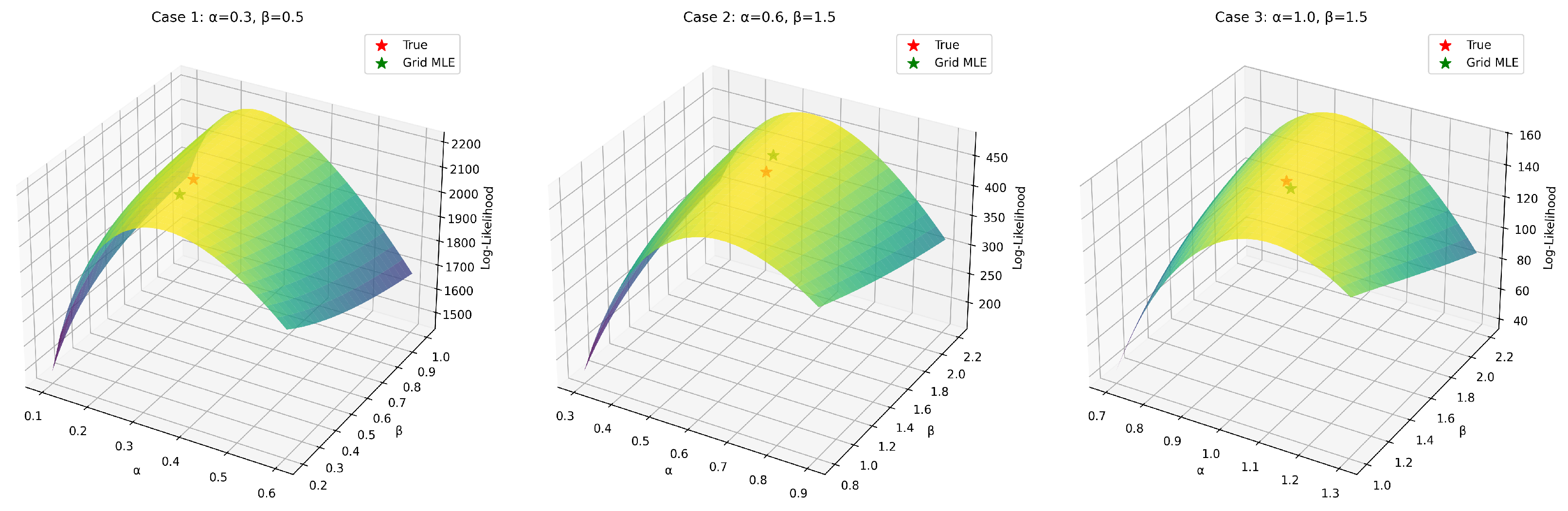
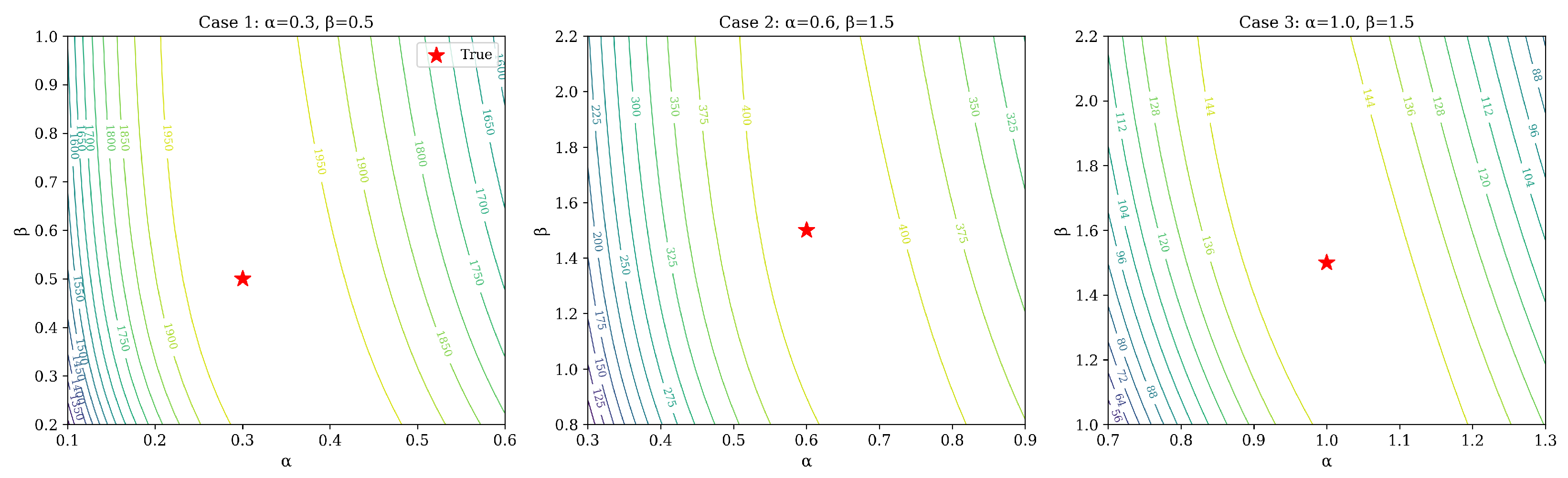
To investigate uniqueness, we performed maximum likelihood estimation from 30 randomly chosen starting points for three representative parameter configurations. Figure 3 and Figure 4 display the log-likelihood surfaces and contours for these configurations.

Table 1. MLE Convergence from Multiple Starting Points for Three Parameter Configurations.

True Parameters	$\widehat{\mathit{\alpha }}$		$\widehat{\mathit{\beta }}$		Success
	Mean (Sth)	Bias	Mean (Sth)	Bias
Case 1: $\alpha =0.3$, $\beta =0.5$	0.3087 (0.0000)	0.0087	0.4129 (0.0000)	−0.0871	30/30
Case 2: $\alpha =0.6$, $\beta =1.5$	0.5787 (0.0000)	−0.0213	1.6365 (0.0000)	0.1365	30/30
Case 3: $\alpha =1.0$, $\beta =1.5$	1.0176 (0.0000)	0.0176	1.4826 (0.0000)	−0.0174	30/30

summarizes the results from multiple starting points. For each configuration, all 30 starting points converged to virtually identical estimates, with standard deviations effectively zero (reported as 0.0000 in the table due to numerical precision). This provides strong empirical evidence of a unique global maximum.

These findings provide strong empirical evidence that the MLE for the UEDTD exists and is unique under standard regularity conditions. The successful convergence from all 30 starting points across different parameter configurations confirms the reliability of the estimation procedure. The zero standard deviations indicate that all starting points converged to identical estimates, further reinforcing the uniqueness property.

6. Simulation Study

A comprehensive Monte Carlo simulation study was conducted to evaluate the finite-sample performance of the maximum likelihood estimators (MLEs) for the UEDTD parameters. average width of confidence intervals, The assessment considered bias, mean squared error (MSE), average width, and coverage probability of 95% and 90% Wald confidence intervals across various sample sizes and parameter configurations using Python 3.9. The study considered sample sizes $n=20, 30, 50, 100, 200, 300, 500$ and four parameter settings: $({\lambda }_1,{\lambda }_2)=(0.3, 0.8)$, $(0.6, 1.0)$, $(1.0, 1.5)$, and $(1.5, 2.5)$. These configurations cover different hazard shapes (U-Shaped when ${\lambda }_1<1$, increasing when ${\lambda }_1>1$) and varying separation between parameters. For each combination, 1000 independent samples were generated from the UEDTD using Algorithm 1 (product of power-function variables), and MLEs were computed via Algorithm 4 (fixed-point iteration) with the reparameterized form $(\alpha ,\beta )$. Confidence intervals were constructed using the observed information matrix and delta method as derived in the previous subsection.

The simulation results are summarized in

Table 2. Simulation results for MLE of UEDTD parameters (${\lambda }_1=0.3$, ${\lambda }_2=0.8$).

				95% CI		90% CI
n	MLE	Avg Bias	MSE	Avg Width	Coverage	Avg Width	Coverage
20	0.3562	0.056193	0.014353	0.7729	0.9609	0.6487	0.9250
	1.3308	0.530778	5.168904	6.2242	0.9187	5.2235	0.8860
30	0.3476	0.047632	0.011078	0.6443	0.9571	0.5407	0.9376
	1.0837	0.283656	1.803853	3.9244	0.9274	3.2934	0.8916
50	0.3440	0.043991	0.008405	0.5175	0.9799	0.4343	0.9608
	0.8681	0.068057	0.328990	2.3165	0.9005	1.9440	0.8482
100	0.3323	0.032340	0.005387	0.3606	0.9760	0.3026	0.9490
	0.8099	0.009919	0.137007	1.4979	0.9260	1.2571	0.8960
200	0.3203	0.020272	0.002607	0.2264	0.9720	0.1900	0.9550
	0.7914	−0.008564	0.054628	1.0066	0.9560	0.8448	0.9410
300	0.3188	0.018761	0.001867	0.1783	0.9870	0.1496	0.9690
	0.7749	−0.025136	0.040503	0.7984	0.9690	0.6700	0.9290
500	0.3160	0.015960	0.001185	0.1288	0.9870	0.1081	0.9690
	0.7628	−0.037166	0.022526	0.6019	0.9600	0.5051	0.9160

,

Table 3. Simulation results for MLE of UEDTD parameters (${\lambda }_1=0.6$, ${\lambda }_2=1.0$).

				95% CI		90% CI
n	MLE	Avg Bias	MSE	Avg Width	Coverage	Avg Width	Coverage
20	0.6446	0.044606	0.034215	1.4564	0.9261	1.2222	0.8935
	1.7341	0.734136	10.946418	7.4462	0.9783	6.2490	0.9707
30	0.6255	0.025501	0.026687	1.2122	0.9097	1.0173	0.8750
	1.4822	0.482157	2.825010	4.9633	0.9905	4.1653	0.9832
50	0.6235	0.023488	0.020058	1.0166	0.9239	0.8532	0.8863
	1.2459	0.245944	0.904396	3.1603	0.9888	2.6522	0.9787
100	0.6292	0.029245	0.013421	0.7940	0.9520	0.6664	0.9329
	1.0829	0.082852	0.169451	1.9420	0.9940	1.6298	0.9780
200	0.6213	0.021272	0.008705	0.6026	0.9500	0.5057	0.9110
	1.0325	0.032455	0.079105	1.3921	0.9900	1.1683	0.9710
300	0.6137	0.013718	0.006712	0.4786	0.9390	0.4016	0.9080
	1.0365	0.036542	0.054299	1.1392	0.9900	0.9561	0.9620
500	0.6133	0.013320	0.005400	0.3768	0.9340	0.3162	0.9110
	1.0179	0.017870	0.036574	0.8876	0.9770	0.7449	0.9420

,

Table 4. Simulation results for MLE of UEDTD parameters (${\lambda }_1=1.0$, ${\lambda }_2=1.5$).

				95% CI		90% CI
n	MLE	Avg Bias	MSE	Avg Width	Coverage	Avg Width	Coverage
20	1.0336	0.033623	0.081447	2.3746	0.9025	1.9929	0.8735
	2.5626	1.062586	12.459730	10.2522	0.9818	8.6039	0.9743
30	1.0295	0.029520	0.060229	2.1395	0.9234	1.7955	0.8825
	2.1568	0.656823	6.952904	7.1724	0.9927	6.0193	0.9853
50	1.0363	0.036329	0.050684	1.7718	0.9149	1.4869	0.8841
	1.8363	0.336284	1.499795	4.6521	0.9877	3.9042	0.9846
100	1.0278	0.027769	0.033062	1.3621	0.9287	1.1431	0.9036
	1.6678	0.167829	0.398216	3.0264	0.9990	2.5399	0.9970
200	1.0245	0.024515	0.022864	1.0519	0.9300	0.8828	0.9080
	1.5755	0.075537	0.179172	2.1354	0.9970	1.7921	0.9830
300	1.0195	0.019548	0.018604	0.8702	0.9400	0.7303	0.9110
	1.5592	0.059207	0.118008	1.7640	0.9960	1.4804	0.9690
500	1.0093	0.009328	0.013191	0.6872	0.9330	0.5767	0.8930
	1.5448	0.044834	0.076120	1.4109	0.9930	1.1840	0.9560

and

Table 5. Simulation results for MLE of UEDTD parameters (${\lambda }_1=1.5$, ${\lambda }_2=2.5$).

				95% CI		90% CI
n	MLE	Avg Bias	MSE	Avg Width	Coverage	Avg Width	Coverage
20	1.6426	0.142612	0.243178	3.8210	0.9125	3.2067	0.8796
	4.2699	1.769896	47.241696	17.0173	0.9683	14.2814	0.9540
30	1.6179	0.117897	0.170454	3.6219	0.9274	3.0396	0.8938
	3.5304	1.030437	16.316190	12.3731	0.9737	10.3838	0.9695
50	1.5940	0.094029	0.129854	2.8145	0.9284	2.3620	0.9029
	2.9938	0.493768	4.163767	7.6538	0.9847	6.4232	0.9765
100	1.5856	0.085614	0.092699	2.1453	0.9310	1.8004	0.9010
	2.7084	0.208355	1.129489	4.9687	0.9960	4.1699	0.9810
200	1.5721	0.072101	0.064027	1.5779	0.9420	1.3242	0.9050
	2.6000	0.100026	0.555716	3.5088	0.9920	2.9447	0.9610
300	1.5590	0.058974	0.050208	1.3125	0.9420	1.1015	0.9140
	2.5396	0.039565	0.399667	2.8728	0.9860	2.4110	0.9410
500	1.5380	0.037964	0.033985	0.9967	0.9270	0.8364	0.9070
	2.5500	0.050010	0.239694	2.2984	0.9720	1.9289	0.9340

. For each sample size, the upper row corresponds to ${\lambda }_1$ and the lower row to ${\lambda }_2$.

For all parameter configurations, bias and MSE decrease monotonically with sample size, confirming consistency of the MLEs. The Small-sample bias ($n=20$–30) is noticeable when ${\lambda }_1$ is small (e.g., Case 1: ${\lambda }_1=0.3$) or when ${\lambda }_2-{\lambda }_1$ is large (e.g., Case 4: ${\lambda }_2-{\lambda }_1=1.0$), with the bias ${\widehat{\lambda }}_2$ reaching $1.770$ in Case 4 at $n=20$. However, bias diminishes rapidly; by $n=50$, relative bias for ${\lambda }_2$ in Case 4 drops to $19.8\%$, and by $n=100$ to $8.3\%$. Configurations with moderate parameter values (Cases 2 and 3) exhibit smaller biases even at small samples.

Coverage probabilities for 95% confidence intervals are generally close to nominal levels ($0.90$–$0.98$) across all sample sizes. Slight undercoverage occurs in some cases at $n=20$–30 (e.g., Case 1 ${\lambda }_2$ coverage $0.9187$ at $n=20$), but improves rapidly, exceeding $0.95$ for $n\ge 200$. The 90% intervals show similar patterns with coverage typically $0.87$–$0.97$.

Average interval widths decrease substantially as n increases, reflecting improved precision. Widths are larger for configurations with smaller ${\lambda }_1$ or larger separation ${\lambda }_2-{\lambda }_1$, consistent with higher variability in those regions. For example, the 95% CI width for ${\lambda }_2$ in Case 4 narrows from $17.02$ at $n=20$ to $2.30$ at $n=500$, a $86\%$ reduction.

Overall, the MLEs and associated Wald intervals perform reliably across all configurations, with good small-sample behavior in most cases and rapid convergence to asymptotic properties as n grows. These results support the practical use of the proposed estimation procedures.

7. Data Analysis

In this section, we demonstrate the practical applicability of the proposed distribution through a comprehensive data analysis using a real-world dataset. We examine the fitting performance of the UEDTD, comparing the results with other well-known distributions.

The dataset represents relative humidity data from the Haarweg Wageningen weather station in the Netherlands in May 2007, as reported in meteorological studies. The data represents the relative humidity of surface air and has been recently examined by Rahman [26] and previously by Raschke [27] and Yao [28], where the beta distribution has traditionally been applied. The data consist of 30 measurements scaled to the unit interval (divided by 100), as presented in

Table 6. Relative Humidity Dataset (May 2007).

0.40	0.44	0.50	0.55	0.58	0.62	0.65	0.69	0.72	0.72
0.73	0.75	0.77	0.80	0.81	0.81	0.83	0.83	0.85	0.85
0.85	0.86	0.86	0.87	0.87	0.89	0.92	0.94	0.94	0.97

.

Table 7. Goodness-of-fit comparison for different unit distributions (Relative Humidity Dataset).

Distribution	Parameters	Log-Lik	AIC	BIC	KS D	KS p-Value
UEDTD	(4.7391, 12.0851)	18.88	−33.77	−30.97	0.1029	0.8765
Kumaraswamy	(5.2866, 2.1212)	18.88	−33.76	−30.96	0.1078	0.8399
Beta	(6.1722, 1.9412)	18.76	−33.52	−30.72	0.1138	0.7910
Unit−Gamma	(1.9342, 6.5844)	18.75	−33.51	−30.71	0.9848	0.0000
Two−sided Power	(0.9400, 3.0057)	18.55	−33.11	−30.31	0.1385	0.5654
Unit Weibull	(1.4138, 4.9029)	18.21	−32.42	−29.62	0.1220	0.7178
Topp−Leone	(11.4600)	17.18	−32.37	−30.97	0.1930	0.1873

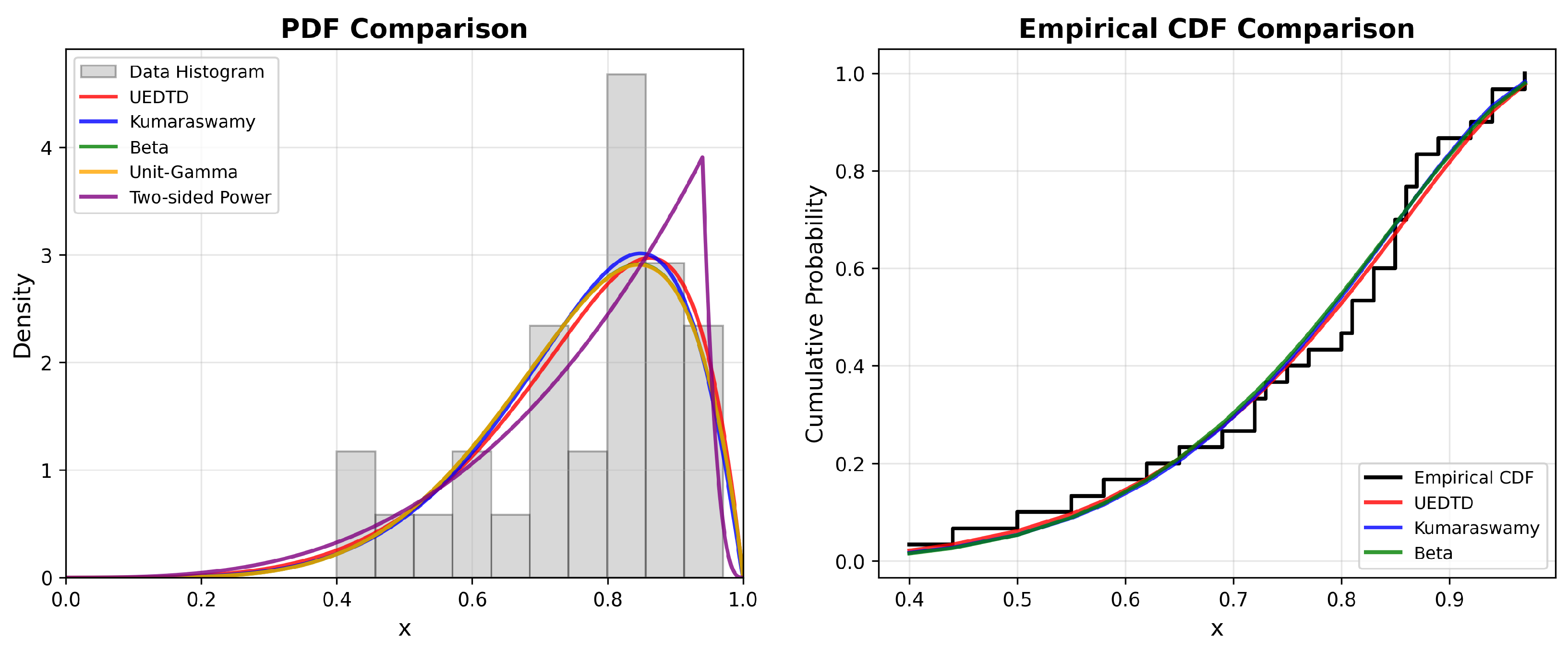
presents the fitting results for the relative humidity dataset. The UEDTD demonstrates strong performance, achieving the lowest AIC (−33.77) and BIC (−30.97) among all models. With a KS statistic of 0.1029 and a p-value of 0.8765, the UEDTD provides an excellent fit to the data. The estimated parameters, along with their confidence intervals, are provided in

Table 8. 95% and 90% Wald CI for the UEDTD parameters fitted to the Relative Humidity dataset.

${\mathit{\lambda }}_{\mathit{i}}$	${\widehat{\mathit{\lambda }}}_{\mathit{i}}$	Variance	90% CI		95% CI
			Interval	Width	Interval	Width
${\lambda }_1$	4.7391	2.3504	[2.2174, 7.2608]	5.0434	[1.7343, 7.7439]	6.0096
${\lambda }_2$	12.0851	72.6015	[−1.9302, 26.1003]	28.0305	[−4.6151, 28.7853]	33.4003

. The covariance matrix below also shows the relationship between the estimated parameters.

$$\begin{array}{c}\hfill \mathrm{Cov}({\widehat{\lambda }}_1,{\widehat{\lambda }}_2)=\left(\begin{array}{cc}2.3503890& -10.4159617\\ -10.4159617& 72.6015102\end{array}\right)\end{array}$$

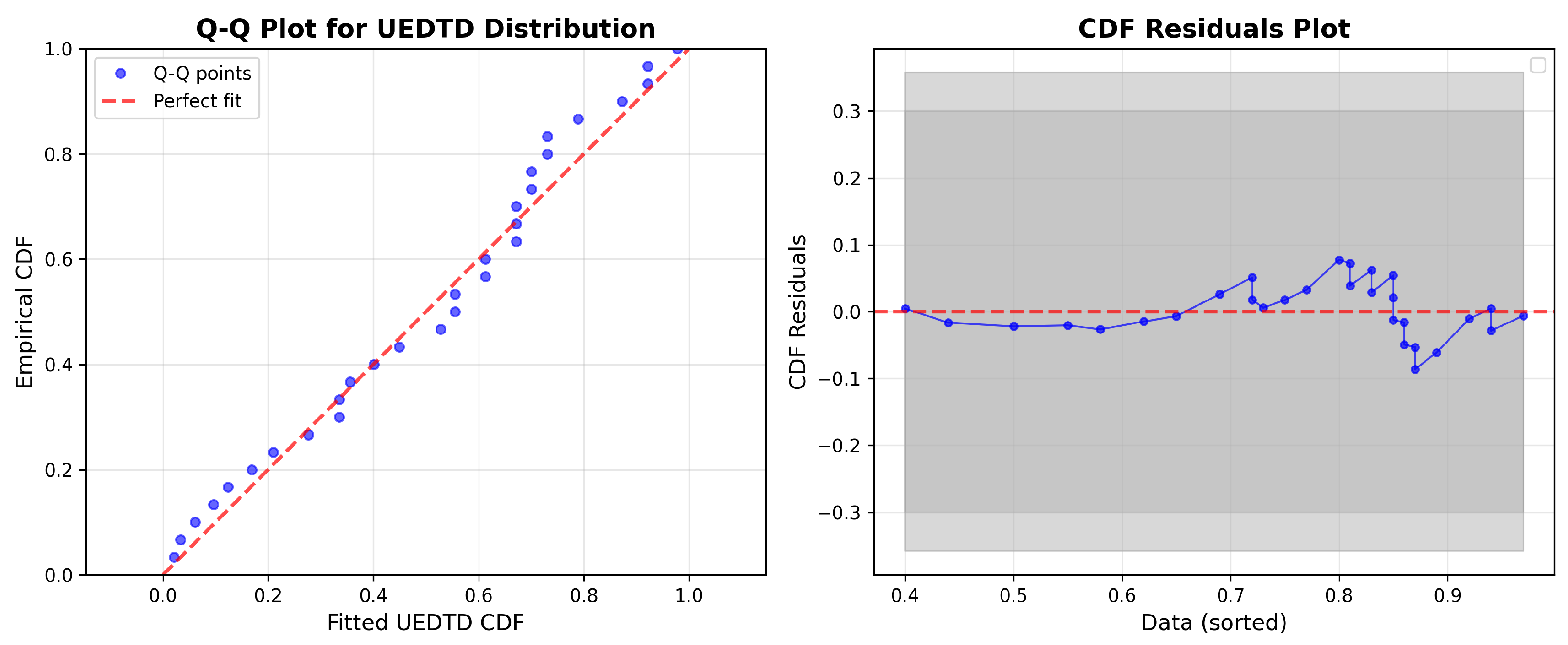
The visual comparison in Figure 5 shows that the UEDTD captures the distribution of relative humidity percentages effectively. The diagnostic plots presented in Figure 6 confirm the model’s appropriateness for the dataset.

8. Conclusions

This paper introduced the Unit Exponential Delay Time Distribution (UEDTD), a two-parameter model designed for proportional data bounded within the unit interval $(0,1)$. The distribution was derived through two different approaches: the transformation $Y=e^{-X}$ applied to the Exponential Delay Time Distribution, and as the product of two independent power-function random variables that connects it with Pareto distribution, providing additional interpretability. Given the multiple representations of the UEDTD, we presented two exact and efficient algorithms for generating random samples. The limiting distribution further connected UEDTD with a well-established model, unit-Gamma distribution. We derived key statistical properties, established asymptotic results for extremes as the sample minimum was shown to converge to a Weibull distribution under appropriate normalization, while the maximum gap from the upper bound follows a Rayleigh limit, offering practical insight into tail behavior for reliability applications. For inference, we proposed a reparameterization to enhance the stability of maximum likelihood estimation. A simulation study has been conducted to assess the performance of the estimators. The results confirm that the MLEs are consistent and efficient across different sample sizes and parameter settings. The practical value of the UEDTD was demonstrated through a real-world dataset of relative humidity measurements, where it showed superior performance compared to established unit distributions such as the Beta and Kumaraswamy. Future work could extend the model to regression settings, Bayesian frameworks, or multivariate applications, and consider additional real-data applications across diverse fields.

References

- Christer, A.H. Delay time model of reliability of equipment subject to inspection monitoring. J. Oper. Res. Soc. 1987, 38, 329–334. [Google Scholar] [CrossRef]
- Christer, A.H.; Waller, W.M. Reducing production downtime using delay-time analysis. J. Oper. Res. Soc. 1984, 35, 499–512. [Google Scholar] [CrossRef]
- Christer, A.H.; Waller, W.M. An operational research approach to planned maintenance: Modelling PM for a vehicle fleet. J. Oper. Res. Soc. 1984, 35, 967–984. [Google Scholar] [CrossRef]
- Attia, A.F. Estimation of the reliability function using the delay-time models. Microelectron. Reliab. 1997, 37, 323–327. [Google Scholar] [CrossRef]
- Oguntunde, P.E.; Odetunmibi, O.A.; Adejumo, A.O. On the sum of exponentially distributed random variables: A convolution approach. Eur. J. Stat. Probab. 2014, 2, 1–8. [Google Scholar]
- Mazucheli, J.; Menezes, A.F.B.; Fernandes, L.B.; de Oliveira, R.P.; Ghitany, M.E. The unit-Weibull distribution as an alternative to the Kumaraswamy distribution for the modeling of quantiles conditional on covariates. J. Appl. Stat. 2019, 47, 954–974. [Google Scholar] [CrossRef]
- Sarhan, A.M.; Sobh, M.E. Unit exponentiated Weibull model with applications. Sci. Afr. 2025, 27, e02606. [Google Scholar] [CrossRef]
- Bantan, R.A.R.; Jamal, F.; Chesneau, C.; Elgarhy, M. Theory and applications of the unit gamma/Gompertz distribution. Mathematics 2021, 9, 1850. [Google Scholar] [CrossRef]
- Mazucheli, J.; Menezes, A.F.B.; Ghitany, M.E. The unit-Weibull distribution and associated inference. J. Appl. Probab. Stat. 2018, 13, 1–22. [Google Scholar]
- Korkmaz, M.Ç; Chesneau, C. On the unit Burr-XII distribution with the quantile regression modeling and applications. Comput. Appl. Math. 2021, 40, 29. [Google Scholar] [CrossRef]
- Haq, M.A.U.; Hashmi, S.; Aidi, K.; Ramos, P.L.; Louzada, F. Unit modified Burr-III distribution: Estimation, characterizations and validation test. Ann. Data Sci. 2023, 10, 415–440. [Google Scholar] [CrossRef]
- Sarhan, A.M. Unit-Chen distribution and its quantile regression model with applications. Sci. Afr. 2025, 27, e02555. [Google Scholar] [CrossRef]
- Altun, E. The log-weighted exponential regression model: Alternative to the beta regression model. Commun. Stat. Theory Methods 2021, 50, 2306–2321. [Google Scholar]
- Altun, E.; Hamedani, G.G. The log-xgamma distribution with inference and application. J. Soc. Fr. Stat. 2018, 159, 40–55. [Google Scholar]
- Bantan, R.A.R.; Chesneau, C.; Jamal, F.; Elgarhy, M.; Tahir, M.H.; Aqib, A.; Zubair, M.; Anam, S. Some new facts about the unit-Rayleigh distribution with applications. Mathematics 2020, 8, 1954. [Google Scholar] [CrossRef]
- Ratnaparkhi, M.V.; Mosimann, J.E. On the normality of transformed beta and unit-gamma random variables. Commun. Stat. Theory Methods 1990, 19, 3833–3854. [Google Scholar] [CrossRef]
- Grassia, A. On a family of distributions with argument between 0 and 1 obtained by transformation of the gamma and derived compound distributions. Aust. J. Stat. 1977, 19, 108–114. [Google Scholar] [CrossRef]
- Scheffé, H. A useful convergence theorem for probability distributions. Ann. Math. Statist. 1947, 18, 434–438. [Google Scholar] [CrossRef]
- Gnedenko, B.V. Sur la distribution limite du terme maximum d’une série aléatoire. Ann Math. 1943, 44, 423–453. [Google Scholar] [CrossRef]
- Beirlant, J.; Goegebeur, Y.; Segers, J.; Teugels, J. Statistics of Extremes: Theory and Applications; Wiley: Hoboken, NJ, USA, 2004. [Google Scholar]
- de Haan, L.; Ferreira, A. Extreme Value Theory: An Introduction; Springer: Berlin/Heidelberg, Germany, 2006. [Google Scholar]
- Gomes, M.I.; Guillou, A. Extreme value theory and statistics of univariate extremes: A review. Int. Stat. Rev. 2015, 83, 263–292. [Google Scholar]
- Albrecher, H.; Beirlant, J.; Teugels, J.L. Reinsurance: Actuarial and Statistical Aspects; Wiley: Hoboken, NJ, USA, 2017. [Google Scholar]
- Arnold, B.C.; Balakrishnan, N.; Nagaraja, H.N. A First Course in Order Statistics; SIAM: Philadelphia, PA, USA, 2008. [Google Scholar]
- Casella, G.; Berger, R.L. Statistical Inference, 2nd ed.; Duxbury Press: Pacific Grove, CA, USA, 2002. [Google Scholar]
- Rahman, M.; Amin, M.I.; Hasan, M. A note on beta distribution goodness of fit. Open J. Stat. 2025, 15, 35–40. [Google Scholar] [CrossRef]
- Raschke, M. Empirical behaviour of tests for the beta distribution and their application in environmental research. Stoch. Environ. Res. Risk Assess. 2011, 25, 79–89. [Google Scholar] [CrossRef]
- Yao, A.Y.M. A statistical model for the surface relative humidity. J. Appl. Meteorol. 1974, 13, 17–21. [Google Scholar] [CrossRef]