Article

Modeling the Energy Consumption of a Public Blockchain as a Stochastic Process

by
Victor D. Cruz-González
1,*,
Héctor Benítez-Pérez
2 and
Rocío Aldeco-Pérez
3
1
Posgrado en Ciencia e Ingeniería de la Computación, Universidad Nacional Autónoma de México (UNAM), Mexico City 04510, Mexico
2
Instituto de Investigaciones en Matemáticas Aplicadas y en Sistemas (IIMAS), Universidad Nacional Autónoma de México (UNAM), Mexico City 04510, Mexico
3
Facultad de Ingeniería, Universidad Nacional Autónoma de México (UNAM), Mexico City 04510, Mexico
*
Author to whom correspondence should be addressed.
Mathematics 2026, 14(13), 2282; https://doi.org/10.3390/math14132282
Submission received: 20 May 2026 / Revised: 18 June 2026 / Accepted: 23 June 2026 / Published: 26 June 2026

Abstract

In this paper, we propose a multilevel stochastic model for the energy consumption of public proof-of-work blockchains. The main novelty is the proposal of a closed form for the expected energy consumption in one proof of work mining round. In the case of homogeneous per-hash efficiency, this proposition shows that the expected spending is e 0 / p depending only on the protocol difficulty and not on the distribution of the hash power among the miners. The proposal connects three levels of analysis: a local model of mining at the node level, a semi-global model of competitive block discovery and propagation, and a global stochastic model of workload, computational capacity, network connectivity and power consumption. This leads to the above closed form energy result. The mining process is approximated locally by exponential waiting times of Bernoulli hash trials. This extends to the semi-global model where the competition among miners and the delay in the propagation lead to the wasted computation. The global layer is modeled as a set of stochastic differential equations which models the interaction between workload dynamics, capacity constraints and communication overheads. The core analysis does not need Bayesian or Markov decision components but these are recommended for modeling estimation and adaptive control. We start with preliminary simulations on the VIBES platform and find qualitative properties of the full model: the total energy cost scales roughly linearly with the size of the network, the average energy per node decreases with increasing network size, the propagation latency is the primary source of wasted computation due to stale blocks and nodes tend to operate in a capacity-depleted regime with the workload-induced degradation being substantially higher than the recovery rate. The results give a structural analysis of how the design of the protocol and the network conditions affect the energy consumption and emphasize the importance of quantitatively calibrating with empirical data from Bitcoin.
MSC:
60J20; 60H10; 90C40; 62F15; 68M20

1. Introduction

Public blockchains are shared ledgers that are not centrally controlled. They require a distributed set of nodes to validate, store and propagate the same information. In proof-of-work (PoW) systems this process is inherently competitive; multiple miners run repetitive hash computations on candidate blocks, but only one valid block is eventually added to the chain [1,2]. That means a large portion of the computational power used by the network is not directly working toward the final state ledger. The energy consumption thus is not incidental but a structural feature of the protocol.
This phenomenon has been widely reported. Empirical studies [3,4,5,6,7] estimate the total energy consumption, carbon emissions and energy per block for major PoW networks such as Bitcoin. The work gives valuable quantitative benchmarks and environmental relevance of public blockchain infrastructures. Yet, most existing approaches rely on aggregate indicators (e.g., total hashrate or annual energy use) and do not explicitly model the stochastic processes underlying how local node behavior and network interactions give rise to system-wide energy consumption.
This restriction encourages a more detailed analytical approach. The energy in PoW blockchains is due to a mix of processes at different scales: individual nodes locally hash and validate, groups of nodes compete to find blocks with network delays and the entire system evolves as workload, computational capacity and connectivity change. Such a modeling framework that does not discriminate these levels cannot readily explain to what extent different sources of energy expenditure (e.g., competitive overlap, propagation delays, or workload congestion) contribute to the total.
The goal of this paper is the development of a multilevel stochastic framework linking these scales in a consistent and analytically treatable manner. The main gap addressed here is the lack of an integrated model that formulates and studies local mining dynamics, semi-global block races and the evolution of global system states jointly in terms of their energetic implications. This limitation results in three concrete research questions that drive the current work. First, what is the expected energy consumed in a single round of proof-of-work mining, as a function of the protocol difficulty and the hardware efficiency? Second, how does propagation delay turn valid local work into globally wasted computation, and how large is that waste relative to the total? Third, can the continuous-time evolution of workload, computational capacity and network connectivity be formalized in a unified stochastic framework that connects local mining behavior to aggregate energy expenditure? The present paper answers all three questions in a single multilevel modeling framework.
The proposed approach is structured in three levels. The local level describes the mining process of a single node. The semi-global level captures the competition between miners and energetic effects of block propagation. The global level characterizes the evolution of workload, available computational capacity, network connectivity and power consumption. This decomposition is analytically clean: it separates the physical location of energy use from the network mechanisms that determine when that use is useful or wasteful. Together, these levels allow us to differentiate accepted work from wasted competitive effort, and to understand blockchain energy as the outcome of dynamic interactions, rather than a static by-product of hash rate.
The rest of this paper is organized as follows. Related literature on the stochastic methods and the energy modeling of the blockchain is summarized in Section 2. In Section 3, we develop the conceptual perspective of blockchain as an operationally closed system. The notation and modeling assumptions are presented in Section 4. In Section 5, we introduce the multilevel stochastic framework at local, semi-global and global levels. Extensions based on Bayesian and MDP are presented in Section 6. Section 7 deals with global energy implications; for example, expected total energy and operating regimes. Section 8 introduces the structural view of the global model, stability analysis and sensitivity. Section 9 presents results from the VIBES simulations. We end with limitations and future work in Section 10.
This paper proposes a local exponential-race model for PoW mining, derives a closed-form formula for the expected energy of one mining round (assuming homogeneous per-hash efficiency) and incorporates that result into an explicit-state global stochastic framework. We retain modular extensions of Bayesian estimation of latent mining intensity, and a Markov Decision Process (MDP) formulation of operational choices. Preliminary simulations performed with the VIBES platform then show how the framework takes into account scaling properties, propagation-related waste and the state-dependent nature of energy consumption per node.

2. Background and Related Work

2.1. Operational Components of Public PoW Blockchains

For energy analysis, three components are particularly important. The first is the mining itself, PoW. In systems such as Bitcoin, miners repeatedly change a nonce until the cryptographic hash of the block header is less than a target derived from the network difficulty [1]. Each trial is cheap computationally, but expensive in total because the network relies on a very large number of repeated trials. The second part is the UTXO accounting model, where transactions consume previous outputs and create new ones. The process of creating, verifying, storing and relaying UTXOs that happen in parallel with mining [2] incurs local processing and communication costs. The third is through peer-to-peer dissemination. Transactions and blocks are propagated via gossip-like overlays where nodes verify messages and relay them to neighbors, which introduces some redundancy that makes the system more robust, but involves more communication [8].
These components interact in non-trivial ways. Propagation is not instantaneous, so two miners can satisfy the proof-of-work condition nearly simultaneously and create temporary competing branches before the network converges. The stale blocks produced do not affect performance; they represent actual energy expended on branches that do not make it into the canonical chain [9,10]. Furthermore, transaction load is not energetically neutral. The nodes with higher workload need to validate more data, manage larger mempools and endure longer communication activity, which can all affect their available capacity for mining.
Hence, a public blockchain is an operationally closed system. Once value is represented in the ledger, any transfer must then necessarily be validated, propagated and agreed upon. Participants are both users and caretakers of the same infrastructure. Redundancy is what gives the protocol its trust, but that redundancy increases the amount of computations and messages needed to receive a single accepted outcome.

2.2. Energy Literature

The energy consumption of blockchain has been dealt with in empirical, macroeconomic and hardware-oriented literature. O’Dwyer and Malone [11] provided the first quantitative estimates of the electricity footprint of Bitcoin and Vranken [12] contextualized these figures within a broader sustainability perspective. The most prominent strand remains macroeconomic: De Vries [3,13] links electricity consumption to mining profitability and market incentives; Prat and Walter [14] propose an equilibrium model of the Bitcoin mining market in which hash rate is endogenously determined by the exchange rate under free entry, providing a micro-founded basis for the workload dynamics modeled in the present framework; Stoll et al. [4] link it to carbon emissions via regional grid and hardware efficiency data; Jiang et al. [5] study projected growth scenarios under different regulatory conditions; and Bejan et al. [6] investigate the empirical relationship between price dynamics and energy demand. This analysis is extended to multiple PoW currencies by Krause and Tolaymat [15] and the Cambridge Centre for Alternative Finance [7] provides one of the most widely used benchmark datasets. Taylor [16] shows how the move from CPUs to ASICs influenced the energy profile of single nodes at the hardware level and Sedlmeir et al. [17] provide a systematic comparison of consensus mechanisms from an energy perspective. Through the lens of carbon footprint and grid decarbonization, the environmental sustainability of PoW mining has also been studied. Ibañez and Freier [18] systematize the state of knowledge on Bitcoin energy and renewable integration. Li et al. [19] use a CO2 emission projection model to argue that the carbon footprint of PoW requires a structural response at the level of the consensus mechanism itself, a challenge that the present work addresses by providing an analytical framework to decompose where that footprint comes from.
These studies are indispensable but they work mostly with aggregate observables, e.g., total hashing power, network difficulty or yearly consumption. Not only they lack stochastic modeling, but they also do not distinguish between the mechanisms generating the energy consumption: Competitive overlap between miners, propagation delays converting valid work into stale blocks, workload-induced capacity degradation and communication overhead all contribute differently to the total, but aggregate indicators confuse them. Without accounting for these components, it is hard to grasp how protocol design choices or network conditions can change the balance between them.
This work also contributes analytically to the fact that energy modeling must not ignore hardware heterogeneity, dynamic profitability and infrastructure effects such as cooling or power usage effectiveness. This is also backed by studies into energy-efficient alternatives like Green-PoW [20] and EPoW [21], which demonstrate that substantial waste reductions necessitate intervention at the level of competitive dynamics, rather than solely at the level of hardware efficiency. Work on energy-aware consensus for constrained networks such as that by Wadhwa et al. [22] quantifies the energy cost of the consensus mechanism as a function of the number of nodes and offloading strategy, motivating the need for a model that endogenizes the relationship between network size, computational capacity and energy expenditure. The present article is not meant to replace aggregate estimates. Instead, it provides a process-oriented structure relating local mining behavior, semi-global competition and global state evolution, in which those estimates can be fitted later for calibration.

2.3. Stochastic Modeling and Remaining Gap

Stochastic methods have been used to analyze blockchain systems along several different lines, each of which targets a different aspect of the protocol behavior. This mining process is described at the local level by Bernoulli trials, and their exponential-time limit [23]. This representation has been used to analyze strategies for selfish mining [24,25,26]. Piazza et al. [26] provide an efficient algorithm for proportional lumpability of Markov chains applied to the selfish mining problem, which can be seen as a formal computational counterpart of the Markovian structure used in the present local-level model and pool reward mechanisms [27,28]. At the network level, block arrival and propagation has been modeled with Poisson processes and queuing theory: Bowden et al. [29] analyze block inter-arrival times in competitive mining. Kasahara and Kawahara [30] and Kawase and Kasahara [31] employ queueing analysis to the dynamics of transaction confirmation. Decker and Wattenhofer [9] and Croman et al. [10] have studied empirically and analytically the impact of propagation delays on the probability of a fork, showing that communication latency is a first-order determinant of wasted computational effort. More recent work has taken these ideas to energy-aware design: Lasla et al. [20] and Yu et al. [21] propose consensus variants that use stochastic arguments to reduce competitive overlap. The stochastic dynamics of the mining market have also been studied at the macro level: Noda et al. [32] show that the stability of transaction speeds under the difficulty adjustment algorithm of Bitcoin depends on the elasticity of hash supply, and characterize the conditions under which the system converges to a stationary distribution—a result directly relevant to the equilibrium and stationarity analysis in Section 5.5 of the present work. Kawaguchi et al. [33] generalize this to a multi-currency stochastic model of the mining market, and derive analogous stability conditions for transaction speeds to the structural stability conditions derived in Section 8.
One major shortcoming of the present literature as surveyed above is the lack of an integrated framework that simultaneously models local mining dynamics, semi-global block races and the evolution of global system states and studies them in terms of their energetic implications. What they lack is their synthesis in one consistent scheme in which the main quantity of interest is energy. Mathematically, the existing Poisson-process and queueing-theoretic models assume fixed parameters for arrival rates and service capacities. The present framework endogenizes such parameters as stochastic state variables coupled via a system of SDEs. Conceptually, selfish-mining and pool-reward models are concerned with strategic incentives and implicitly treat energy, while the present work focuses on energy consumption as the main quantity of interest and derives it from the joint stochastic dynamics of hashing, propagation, workload accumulation and capacity degradation. Stochastic threshold dynamics are also used in epidemic-economic models to characterize system-level stability [34]. The analytical structure of epidemic-economic models, including the derivation of extinction and persistence conditions based on the eigenvalue analysis of coupled SDEs and the use of Itô–Lyapunov functions, is structurally similar to the stability analysis developed in Section 8 of the present work. They are not about energy. They are about strategic incentives. Selfish mining studies. Queueing models of confirmation time consider capacity as a fixed, not a state variable that degrades under workload. Propagation analyses quantify the fork probability but do not relate it to the aggregate power consumption over time. Network structure and hardware efficiency are thus considered exogenous inputs in energy studies as opposed to being endogenous outcomes of a dynamic system. This results in a patchy picture where the mechanisms that drive energy expenditure are understood in isolation and not as a whole.
This paper fills this gap by constructing a multilevel stochastic framework that explicitly ties the three levels together. The goal is to build a consistent multilevel model that retains enough structure to enable analysis, simulation and eventually calibration against empirical data.

2.4. Research Gap and Novel Contributions

The review above identifies four streams of prior work: (1) aggregate energy estimation using hash rate and profitability. (2) Local mining models based on Bernoulli trials and exponential approximations; (3) Network-level models based on Poisson processes and queueing theory; (4) Propagation analyses that relate latency to fork probability. Each stream considers a different aspect of the problem. However, none of the existing works combines all four streams into a single framework with energy as the main quantity of interest.
This paper attempts to fill this gap in three specific ways. First, it provides a closed-form analytical result (Proposition 1) that quantifies expected round-level energy as a function of difficulty and per-hash hardware efficiency. No result like this in exactly this form is found in the literature cited. Second, it endogenizes the network state variables—workload, computational capacity and connectivity—as stochastic processes coupled via a system of SDEs, rather than as fixed parameters or exogenous inputs. Third, it explicitly links the three levels of analysis: the expected round energy from the local and semi-global layers feeds into the global accumulation process, and global congestion feeds back into local mining intensity through the capacity-to-hash-rate relation.
These contributions differ from existing models in the following ways. Poisson-process and queueing-theoretic models fix capacity as a parameter; the present work makes it a state variable with its own dynamics. The propagation analyses estimate the fork probability, but do not relate it to the aggregate power consumption over time. The present work combines both. Selfish-mining models study strategic incentives, and leave energy implicit; the present work takes energy as the primary quantity, and derives its distribution from the joint dynamics of all components. These differences are documented reference by reference in the qualitative comparison of Table 1.
Table 1 summarizes representative references cited in this article to make the distinction between the previous literature and the contribution of this manuscript explicit.

3. Conceptual Perspective and Architectural Mapping

3.1. Blockchain as an Operationally Closed Value System

Public blockchains are closed value systems: once value is introduced to the ledger, every transfer thereafter must be validated and propagated and finalized by the same protocol stack. This means the distinction between users and maintainers is blurred, as transaction depends on the infrastructure that participants also help sustain, often in return for rewards denominated in the native asset. In this structure, energy consumption is not a side cost but part of the operational necessity: the network uses energy to keep the rules in place that allow value to be moved around on the chain, all the time.
This view is important for modeling, since it challenges a purely transactional view of energy use. A blockchain is not only using energy when a transaction is finally recorded. It spends energy all the time to keep the conditions under which transactions can be accepted later at all. Mining, relay, validation and storage are thus not independent service layers stacked one on top of another. They are mutually reinforcing activities in the same closed operational loop.

3.2. Trust, Redundancy and Efficiency

Public blockchains rely on protocol-level redundancy, instead of trusted intermediaries. Many nodes check the same information, propagate it over many paths and store it in many local states. This redundancy is the source of robustness, but also the source of energetic inefficiency. This is not because it is poorly engineered, but because the system builds trust in a decentralized way by repeating and cross-checking work that would be performed once in a centralized architecture.
Therefore, it is useful to speak of a trust-efficiency trade-off, if this phrase is understood qualitatively and not as a literal algebraic law. The more redundancy we have, the more resilient we are to adversarial behavior and local failures, but we have to perform more computation and communication per accepted result. The trade-off is obvious especially in the case of PoW, where the protocol requires many concurrent participants to expend energy, only for one to be the winner. The greater the competitive overlap, the more the system’s security logic seems to be strengthened, but the greater the energetic share of unsuccessful effort becomes.

3.3. Forest of Communication Graphs

At any given moment, a public blockchain is more accurately described as a set of interconnected local state machines rather than a single, coherent global graph. Each node updates its own local state, by validation, relay and mining events, while exchanging messages with neighboring nodes. Since these transitions are asynchronous, the nodes may temporarily have different views of transactions and candidate blocks. Consensus slowly aggregates these local states into one canonical chain. A large portion of the protocol energy is consumed in these transient divergences when computation and communication are performed over competing local views.
The advantage of this model is that it offers an intuitive link between communication delay and energy. When there are multiple candidate blocks at the same time during propagation, miners keep mining on branches that will later disappear and relayers keep relaying information that will soon be useless. So the network is not just a passive means of transmission of blocks that have already been determined. It is a distributed process and local views are temporarily inconsistent. This discrepancy causes additional energy consumption.

3.4. Energy Sources by Scale

The system can be described by the way in which energy is supplied to it at each analytical level. Table 2 presents a consolidated representation of this interpretation.
This model describes the analytical function of each scale. If the goal is to analyze the energy consumption of a single node, the analysis has to be started at the local layer. The semi-global layer is needed if the intention is to consider stale blocks and competitive overlap in block discovery. The global layer is essential if you want to assess the combined impact of workload, computational capacity and connectivity over time. Thus, it is not possible to capture all these dynamics at once with one scalar estimate of annual energy consumption.

4. Notation and Modeling Assumptions

Before presenting the full model, we first discuss the key variables that form the structure of the analysis. The first group corresponds to the local and semi-global levels, where the key quantities are the success probability per attempt, the mining intensity induced by the hash rate, and the stopping time related to the round-level competition. The second group is at the global level where the central state variables are the workload, the available computational capacity, the connectivity and the power. The main notation used throughout this document is presented in Table 3 and Table 4.
The proposed model relies on three common assumptions. First, the PoW block discovery process is a low probability event on a per-hash basis, and so Bernoulli hash attempts are approximated by an exponential waiting-time model in continuous time. Second, we assume the miners are conditionally independent within a given round of competition. This leads to a tractable expression for the minimum stopping time. Third, the global state variables are restricted to physically admissible domains: the workloads and UTXO counts are non-negative, the computational capacities are bounded and the aggregate connectivity is in [ 0 , 1 ] . These assumptions are idealized but they are standard and they provide a coherent basis for an interpretable and operational model.
Table 5 classifies the model’s assumptions according to their role: tractability assumptions are those whose relaxation would change the mathematical form of a key result, while physical approximations are those that simplify the representation of the phenomenon but whose relaxation is in principle feasible without restructuring the framework.
Table 5. Classification of model assumptions by role.
AssumptionTypeConsequence If Relaxed
i.i.d. Bernoulli hash attempts with probability pTractabilityWithout i.i.d., the waiting time does not converge to the exponential law and Proposition 1 requires a more general first-passage distribution
Independent exponential clocks T i Exp ( μ i ) TractabilityWith dependencies, the round stopping time T does not admit a closed-form exponential minimum; the winner probability formula also changes
Homogeneous per-hash efficiency ( ρ i = e 0 h i ( r ) )TractabilityWith heterogeneous efficiency, the expected round energy becomes e ¯ / p where e ¯ is the hash-rate-weighted mean efficiency (see extended Remark in Section 5)
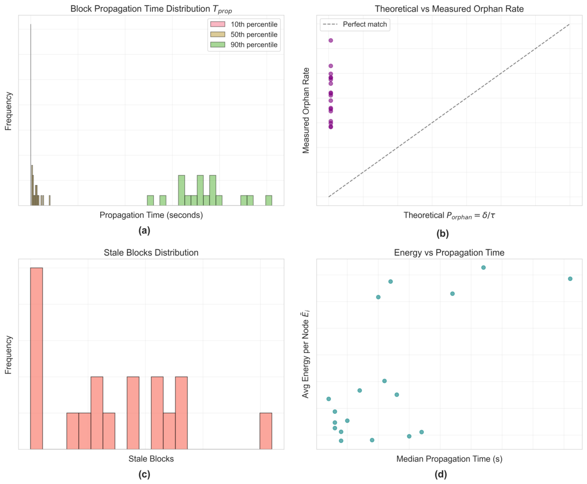
First-order orphan-block approximation P orphan δ prop / τ Physical approximationSimultaneous mining events not captured by the Poisson argument inflate the observed fork rate above the first-order prediction, as confirmed by simulation (Figure 1)
Aggregate connectivity scalar g ( t ) Physical approximationWithout this reduction, the state vector requires tracking the full adjacency matrix; the graph-Laplacian coupling in Section 8.3.3 provides a partial extension
Diagonal diffusion matrix Σ TractabilityCorrelated noise across nodes would modify the covariance structure of total energy (Section 7), requiring an off-diagonal diffusion term

5. Multilevel Stochastic Formulation

5.1. Multilevel Interpretation

A public blockchain is not only a ledger but a temporally growing family of competing propagation trees. Transactions and candidate blocks are introduced into the network, propagate across the peer-to-peer overlay, and overlap until consensus collapses this multiplicity into one accepted chain. This is a useful perspective because it helps to clarify that energy is spent not only on the established history, but also on the maintenance of the temporary forest of alternative trajectories of communication and validation out of which that history emerges.
Our model thus identifies three coupled levels, illustrated in Figure 2. At the local level, each node hashes, validates, stores and relays data. At the semi-global level, nodes interact through block races, propagation and temporary inconsistencies. At the global level, an external observer observes aggregated variables, e.g., throughput, stale blocks, workload, connectivity, energy.

5.2. Local Mining Dynamics

Let r be a mining round and h i ( r ) the hash rate of node n i . Each attempt succeeds if the hash of the candidate block is less than the current target d r = 2 256 k . Under the usual pseudorandomness assumption of SHA-256, the success probability of a single try is
p = Pr SHA 256 ( block ) < d r d r 2 256 = 2 k .
If the node performs h i ( r ) t attempts in a time interval of length t, then the probability of at least one success is
Pr ( T i t ) = 1 ( 1 p ) h i ( r ) t .
For realistic difficulty values, p is notably small, while the number of trials is large. The time to success under the standard rare-event approximation converges to an exponential law:
T i Exp ( μ i ) , μ i = h i ( r ) p .
Equation (3) is the foundation of the local level framework. It keeps the attempt-level logic of PoW but uses a compact continuous-time clock instead of a very large number of Bernoulli trials. In other words, the description in terms of discrete-time Markov chains is conceptually retained but the exponential approximation is used as the effective analytical model.
This local representation shows already one important point about energy. The process is even driven by a deliberately low success probability per-hash to keep the target block interval, set by protocol difficulty, even without considering interaction with other nodes. The protocol is partly secure because success is rare, but this rarity means that each miner has to be active for long periods of time with no guarantee of payment. As mentioned before, local energy expenditure is therefore inseparable from protocol design.
We obtain a local interpretation by modeling mining as a discrete-time Markov chain in which each state corresponds to one more failed hash attempt and success is absorbing. If X i is the number of attempts by node i until success, then
X i Geom ( p ) , E [ X i ] = 1 p .
If each trial takes about 1 / h i ( r ) seconds, then the corresponding waiting time is T i X i / h i ( r ) . In the rare event scaling where p 0 while h i ( r ) p is kept finite, the geometric waiting time converges to the exponential law (3). This is an important observation in the sense that it shows that the continuous-time model is not an arbitrary simplification, it is the limiting form of a discrete attempt-by-attempt delineation.
The discrete representation also makes clear the role of protocol difficulty. Since E [ X i ] = 1 / p , the effect of increased difficulty is not only to reduce the frequency of block arrivals, but also to increase the expected number of hash attempts that fail before the next successful one. These additional tries have real computational and energy costs. Difficulty therefore controls both the expected rate of block-generation and the amount of redundant computation required per accepted block.

5.3. Semi-Global Competition and Propagation

Let H r be the active miners in round r. If each miner carries an independent exponential clock as in (3), then for node n i
T i Exp ( μ i ) , T i Exp ( ϵ i ) , ϵ i = j H r { i } μ j .
Hence, the probability that node n i wins the race is
Pr ( T i < T i ) = μ i μ i + ϵ i = h i ( r ) j H r h j ( r ) .
The winning probability is therefore proportional to hash-rate share. The expected time until the round is resolved is the expectation of the minimum clock,
E [ T ] = 1 j H r μ j = 1 p j H r h j ( r ) .
At this semi-global level, the inefficiency of PoW is fully apparent. All active miners consume energy until the first success, but only one block is accepted; the other part of the expenditure is real although it is not in the canonical chain. The following proposition captures the idea.
Proposition 1.
Consider one mining round with active set H r . Suppose that each node n i H r mines continuously until the first valid block is found, with discovery time T i Exp ( μ i ) independently of the others. Let ρ i > 0 be the power consumption rate of node n i while mining, and let
T = min j H r T j .
Then, the expected total energy consumed in the round is
E [ E r ] = i H r ρ i i H r μ i .
If each hash attempt costs a constant amount of energy e 0 and node n i hashes at rate h i ( r ) , so that ρ i = e 0 h i ( r ) and μ i = h i ( r ) p , then
E [ E r ] = e 0 p = e 0 2 k .
Therefore, assuming homogeneous per-hash efficiency, the expected energy of a PoW round depends on the difficulty and the per-hash hardware efficiency, but not on how the total hash power is distributed among miners.
Proof. 
Because the minimum of independent exponential random variables is itself exponential with rate i H r μ i , we have
E [ T ] = 1 i H r μ i .
During the interval [ 0 , T ] , all active nodes consume energy at their respective rates, so
E r = i H r ρ i T .
Taking expectations proves (9). Substituting ρ i = e 0 h i ( r ) and μ i = h i ( r ) p gives (10).    □
Remark 1.
Equation (10) determines a clean analytical regime. Changing the distribution of hash power among miners changes the winners and losers, but does not change the expected round-level energy as long as the per-hash efficiency is homogeneous. This distinction is useful because discussions of blockchain energy often merge the distribution of rewards with the distribution of expenditures.
If the efficiency is heterogeneous, e.g., if newer generations of ASICs co-exist with older hardware at different J/hash ratios, the derivation has to be adapted. Let e i be the energy cost per-hash of node i. Then, ρ i = e i h i ( r ) and μ i = h i ( r ) p . Then, the expected round energy is
E [ E r ] = i H r e i h i ( r ) i H r h i ( r ) p = e ¯ p ,
where e ¯ = i e i h i ( r ) / j h j ( r ) is the hash-rate-weighted average of the per-hash efficiency of the active miners. Thus, the expected energy per round is e ¯ / p for heterogeneous efficiency, with the effective efficiency determined by the composition of the active mining pool and not any particular node. That is, if total hash power is held constant, expected round energy increases when efficient hardware is replaced with inefficient hardware at the margin—a result that has direct policy relevance. For the homogeneous case e i = e 0 for all i, we recover Equation (10).
Communication and synchronization also take place on the semi-global level. Let δ prop be a representative block propagation time and τ the desired block time. The probability for stale blocks is given by a first-order approximation:
P orphan δ prop τ .
The expression is obtained as follows. Consider blocks which are placed according to a Poisson process with rate 1 / τ and propagation takes a constant time δ prop . A block is stale if another valid block is found and accepted by the network before the first one has finished propagating, i.e., in the time window [ 0 , δ prop ] . The probability of at least one additional discovery in that window is 1 e δ prop / τ . For δ prop τ , the first-order Taylor expansion gives P orphan δ prop / τ , which is Equation (14). This approximation is the leading order term of an empirical formula used by Decker and Wattenhofer [9]. The above ratio approaches 1 as δ prop τ and the first-order approximation becomes inaccurate. In this case, the full expression P orphan = 1 e δ prop / τ should be used. For fixed δ prop , as τ 0 + the ratio δ prop / τ , a regime where new blocks are produced faster than the network can propagate them, i.e., an unstable limit not considered in this model. The simulation results shown in Figure 1b confirm that the first-order approximation underestimates the observed fork rate, as expected due to the existence of simultaneous mining events that the Poisson argument cannot account for. The Equation (14) is a simple one, but it illustrates the main idea: with the slowing down of the propagation process with respect to the production of blocks, more work is performed on blocks that will eventually be orphaned. In terms of energy, communication latency converts local mining effort into globally wasted computation.
The proposition above also contains a useful decomposition into winner and loser expenditure. If node i wins the round, the winner’s energy is E win , i = ρ i T and the energy used by the unsuccessful miners is E lose , i = j i ρ j T . Therefore,
E [ E win , i i wins ] = ρ i j H r μ j , E [ E lose , i i wins ] = j H r { i } ρ j j H r μ j .
This split makes the inefficiency of PoW explicit: most of the energy expenditure goes to nodes whose work is not included in the final accepted block, even for rounds that end without issue. It is not the unsuccessful players that differ from round to round, but the winner.
Another consequence of the exponential-race picture is that the semi-global layer is sensitive to heterogeneity. Heterogeneity in hash power alters the probability of a given node winning, but does not alter expected round-level energy when per-hash efficiency is homogeneous. Heterogenous hardware efficiency, however, changes both the probability of success and the energetic meaning of a given amount of hash power. This is an important distinction for the empirical calibration stage discussed in the Calibration Strategy and Limitations sections, as real blockchain networks are neither hardware-homogeneous nor compositionally static.
The quantities obtained above are defined at the level of a single mining round: a discrete event of random duration ( T ), one winner and a fixed set of losers. The global layer is a result of the continuous accumulation of rounds over time. Blocks are generated with an aggregate rate ( i H r μ i ( t ) ). The total expenditure is the sum of the energy cost of each round. The workload ( Q i ) is the sum of the batches of transactions arriving in the interval and the available capacity ( C i ) is reduced by the ongoing hashing activity. The passage from the semi-global to the global description is not a statistical aggregation, but a time integration. A discrete sequence of competitive races generates continuously evolving state variables whose dynamics must be followed across rounds, rather than within a single round.

5.4. Global State Dynamics

This accumulation process is formalized by the global layer. It is not a single race but a continuous evolution of the workload, capacity, connectivity, and power consumption in each round. The state vector
X t = U t , Q 1 ( t ) , , Q N ( t ) , C 1 ( t ) , , C N ( t ) , g ( t ) ,
where the components are defined in Table 4. This state representation is then utilized to encode the cross-scale feedbacks shaping aggregate energy dynamics via the joint effects of workload, capacity and connectivity.
The functional forms for the drift and diffusion terms are chosen according to three criteria, namely physical boundary consistency, empirical similarity to existing stochastic models in related fields and analytical tractability. The square-root diffusion σ X t on the UTXO population, workload and connectivity processes is the standard Cox–Ingersoll–Ross (CIR) form [35], which is the canonical model for non-negative processes where the variance increases with the level. The SDE drift, λ i ( t ) κ i C i ( t ) , has linear birth–death form, encoding the M/M/1-type queue with state-dependent service rate, directly analogous to the queueing models of Kasahara and Kawahara [30] adapted for continuous time. The capacity degradation term δ i Q i ( t ) + γ i ( C max , i C i ( t ) ) is meant to reflect the intuition that persistent load degrades effective capacity, and idle times allow recovery towards the hardware ceiling, in the spirit of reliability and wear models in operations research. The diffusion factor C i ( t ) ( C max , i C i ( t ) ) is the usual Wright–Fisher type for bounded variables in [ 0 , C max , i ] , which guarantees the disappearance of the volatility at both edges. In Section 9, these forms are partially calibrated empirically, using the results from the VIBES simulation, where the workload-capacity regression gives κ ^ = 14.19 and the analysis of capacity change rate gives δ ^ = 0.000729 and γ ^ 0.00419 .
The UTXO population evolves according to creation and consumption,
d U t = λ create ( t ) μ consume ( t ) d t + σ U U t d W U ( t ) .
The square-root diffusion is used, since the volatility must vanish at the natural boundary U t = 0 . The amount of work at node i is denoted by
d Q i ( t ) = λ i ( t ) κ i C i ( t ) d t + σ Q , i Q i ( t ) d W Q , i ( t ) , Q i ( t ) 0 ,
which models a stochastic queue where arrivals increase the workload and service capacity decreases the workload. The computational capacity available is
d C i ( t ) = δ i Q i ( t ) + γ i ( C max , i C i ( t ) ) d t + σ C , i C i ( t ) ( C max , i C i ( t ) ) d W C , i ( t ) .
Equation (19) formalizes the notion of effective capacity workload degradation, and of recovery during idle times, towards the hardware maximum C max , i .
The local and global layers are coupled through the capacity-to-hash-rate relation
h i ( t ) = h i , max C i ( t ) C max , i , μ i ( t ) = p ( t ) h i ( t ) .
Global congestion feeds back directly to local mining intensity. A heavily loaded node is not only validating and relaying more data, it is also less efficient at mining.
To avoid the necessity of taking the entire adjacency matrix as a state variable, the communication layer is summarized as the following aggregate connectivity process,
d g ( t ) = η g g ¯ ( t ) g ( t ) d t + σ g g ( t ) ( 1 g ( t ) ) d W g ( t ) ,
where g ¯ ( t ) is the instantaneous target connectivity implied by the current network state. This reduced-form representation is sufficient for the present purpose in that it permits communication quality to respond to congestion and recovery, without introducing a high-dimensional graph process in the main equations.
Instantaneous node power is represented by
d P i ( t ) = P base , i + α comp , i Q i ( t ) + α comm , i g ( t ) k i P i ( t ) d t + σ P , i ( Q i ( t ) , P i ( t ) ) d W P , i ( t ) ,
so power contains a baseline term, a workload component, a communication component and a mean-reverting tendency. Total network energy over a horizon [ 0 , T ] is then
E Tot ( T ) = i = 1 N 0 T P i ( t ) d t .
Collecting the state variables gives the compact form
d X t = μ ( X t , t ) d t + Σ ( X t , t ) d W t .
The election of the model in (24) is not just notational. It states explicitly that blockchain energy is state-dependent. The interplay of queue growth, capacity depletion and reduced connectivity have an effect on each other and changes the success probability and instantaneous energetic cost of participation. The model is thus more complete than a description of fixed cost per block, but still compact enough to be simulated or calibrated.
The physically admissible state space is
D X = X t : U t 0 , Q i ( t ) 0 , 0 C i ( t ) C max , i , 0 g ( t ) 1 , i = 1 , , N .
The square-root diffusion factors were deliberately set to zero at the boundaries of this domain. So, when the process hits a physical boundary, it is not kicked out of the admissible set by random fluctuations straightaway. For example, the volatility vanishes at Q i ( t ) = 0 , U t = 0 , and when g ( t ) is at the end points 0 or 1. Similar arguments apply to the capacity term by the factor C i ( t ) ( C max , i C i ( t ) ) .
Boundary compatibility is not sufficient, the drift must point inward at the boundaries. In the present context, it suffices to require
λ i ( t ) κ i C i ( t ) 0 when Q i ( t ) = 0 , δ i Q i ( t ) + γ i ( C max , i C i ( t ) ) 0 when C i ( t ) = 0 ,
with corresponding upper-bound conditions at C i ( t ) = C max , i and g ( t ) = 1 . These inward pointing conditions are standard for diffusion models on constrained domains, and provide a physically meaningful interpretation to the global system: workloads do not become negative, capacity does not exceed hardware limits and connectivity remains a valid fraction.
The global layer can be interpreted as a coupling diagram. Capacity is the effective hash rate. Effective hash rate is the local intensity. Local intensities are the semi-global race. The semi-global race feeds back into workload, propagation and power. Symbolically,
C i ( t ) h i ( t ) μ i ( t ) Pr ( win ) E r E Tot ( T ) .
This direction of dependence is important because it shows what kind of interventions the model is able to study. A change in workload management, hardware efficiency or communication quality is not just a perturbation of a final energy number, but a change of a whole chain of dependent variables.

5.5. Equilibrium and Stationary Behavior

Here, we address the question of existence of stationary solutions or invariant probability distributions for the global SDE system at two levels: deterministic equilibria and stochastic stationarity.
At the deterministic level, the drift equations have an interior equilibrium, which is obtained by setting all drift terms to zero simultaneously. For the workload-capacity subsystem of node i, the equilibrium pair ( Q i , C i ) satisfies λ i = κ i C i and δ i Q i = γ i ( C max , i C i ) , which leads to
C i = λ i κ i , Q i = γ i δ i C max , i λ i κ i .
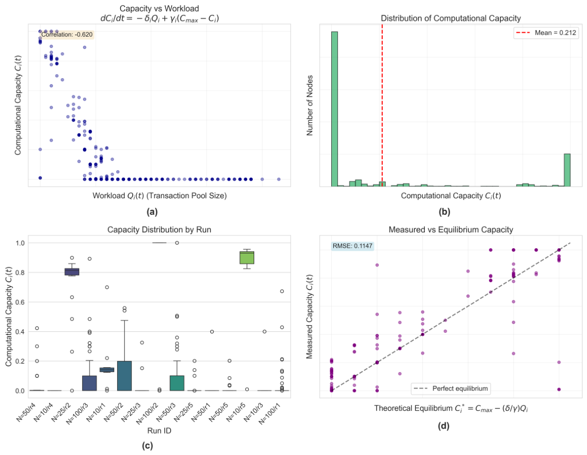
This equilibrium is physically admissible if λ i / κ i C max , i , i.e., when the arrival rate is not greater than the maximum service capacity. As shown in Section 8, the eigenvalues λ i , ± have strictly negative real parts for γ i > 0 , κ i δ i > 0 , and therefore the Jacobian analysis confirms that this equilibrium is locally asymptotically stable. This prediction is supported by the simulation results shown in Figure 3, where we see that even though the nodes are mostly in a capacity-depleted regime, they do not drift indefinitely to the boundary but cluster around C ¯ i = 0.212 , indicating the presence of an attractor in the interior of the state space.
Standard results for diffusions on bounded domain with inward pointing drift at the boundary and non-degenerate diffusion in the interior guarantee the existence of a stationary distribution for the global SDE system at the stochastic level. The square-root diffusion coefficients chosen in the above SDEs satisfy the following conditions: they are zero at the boundaries of D X , so that the process stays in the admissible set, and inward-pointing drift conditions as stated in the admissibility constraints of Section 4 are satisfied by construction. One can show that under these regularity conditions the Fokker–Planck equation corresponding to the global SDE has a stationary solution π ( x ) which satisfies L π = 0 , where L is the adjoint of the infinitesimal generator. We defer characterization of this stationary distribution in closed form to future work, as it is an open problem for the full nonlinear system; however, the numerical evidence from the VIBES simulations is consistent with the existence of a well-defined stationary regime.

5.6. Inference and Control Extensions

The core framework is extended with two optional modules. The first is a Bayesian layer to infer latent mining intensity from local observations. Instead of assuming the node knows its effective rate μ i ( t ) exactly, the node maintains a posterior distribution that is updated from short-window event counts, noisy hash-rate measurements or recent success indicators. This leaves epistemic uncertainty and allows the local competition model to be compatible with imperfect information.
A simple conjugate specification puts a Gamma prior on a latent effective intensity 𝓁 i (distinct from the workload arrival rate λ i ( t ) in the SDE drift) and Poisson distributed short-window event counts. If
𝓁 i Gamma ( a 0 , b 0 ) , Y i , m 𝓁 i Poisson ( 𝓁 i Δ t ) , m = 1 , , M ,
then the posterior remains Gamma,
𝓁 i Y i , 1 : M Gamma a 0 + m = 1 M Y i , m , b 0 + M Δ t .
This kind of layer is useful since it separates the intrinsic protocol randomness and the uncertainty about the node’s own effective state. In practice, a node cannot tell if the lower observed success is due to bad luck, lower capacity or increased competition. In such a case, a posterior distribution contains more information than a point estimate when decisions are to be made.
The second is a Markov Decision Process (MDP) that models operational choices such as mining at full intensity, throttling participation, prioritization of validation, relaying a newly received block or staying idle for a while. s is a node-observable state and a is an admissible action. The energy-aware policy can be summarized using the Bellman equation
V ( s ) = min a c ( s , a ) + γ s P ( s s , a ) V ( s ) ,
where c ( s , a ) penalizes the use of electricity, latency and stale-work risk [36]. The Bayesian part plays a direct supporting role in the framework: the posterior mean E [ 𝓁 i Y i , 1 : M ] provides the estimate of effective mining intensity μ ^ i ( t ) that feeds the local exponential clock and the MDP state. However, the MDP formulation is a modular extension, which demonstrates the architectural completeness of the framework. Its practical contribution is conceptual: it demonstrates that the stochastic model developed at the local and global level offers a natural context in which energy-aware decision rules for individual miners can be formulated and studied. We include below the Bellman equation and the action set only to show that the framework can support such analysis in future work, and not to derive an optimal policy in the present paper. The main analytical results of this paper require no extension.
To make the MDP interpretation concrete, the local observable state is defined as
s t = Q i ( t ) , C i ( t ) , g ( t ) , μ ^ i ( t ) , χ t ,
where μ ^ i ( t ) is the current estimate of mining intensity and χ t encodes protocol events such as receipt of a competing block or successful local propagation. A natural action set is
A = { a mine , a throttle , a validate , a relay , a idle } .
The importance of this extension is conceptual: it shows that the framework does not have to be restricted to passive measurement. It can also be used to study energy-aware participation rules, where a node adjusts its behavior when its workload is high, its capacity is exhausted or its posterior probability of success is too low to justify full-intensity mining.

6. Statistical and Decision Layer

6.1. Bayesian Estimation of Mining Intensity

The competition model is built on a local intensity μ i ( t ) which is not directly observable in practice. Each node has access to noisy proxies of its own state, e.g., recent counts of events, internal performance measures, and delayed information about whether a locally mined block was propagated successfully. Thus, it is natural to have a Bayesian layer, as it regards mining capability as a latent variable, not as a fixed value given from outside.
Let 𝓁 i be the latent effective mining intensity of node i in a short calibration window (different from the workload arrival rate λ i ( t ) in the SDE drift). For a simple conjugate model the prior is
𝓁 i Gamma ( a 0 , b 0 ) ,
and assumes short-window event counts satisfy
Y i , m 𝓁 i Poisson ( 𝓁 i Δ t ) , m = 1 , , M .
The posterior is then
𝓁 i Y i , 1 : M Gamma a 0 + m = 1 M Y i , m , b 0 + M Δ t ,
with posterior mean
E [ 𝓁 i Y i , 1 : M ] = a 0 + m = 1 M Y i , m b 0 + M Δ t .
Then, the posterior mean can be used in the local exponential clock or, more conservatively, the whole posterior distribution can be propagated through the semi-global model. The latter is attractive because it disentangles two sources of randomness that are often conflated in informal discussions: the randomness of mining itself, and the uncertainty a node has about its own effective condition.
The same logic applies to applications in which the node observes noisy hash-rate or performance signals (instead of discrete event counts). The actual probability will vary, but the point of modeling does not. The Bayesian layer takes noisy operational data and produces a probabilistic estimate of the intensity of success, bridging the local hardware uncertainty to the higher-level race model.

6.2. Operational MDP Formulation

The MDP layer describes choice. The Bayesian layer estimates capability. The important thing is that a miner cannot control the outcome of consensus, but it can control how aggressively it plays at a specific point in time. That is a key difference. The PoW winner is random, but the cost of participation in terms of energy consumed is highly dependent on the operational choices made before the winner is known.
The local state is written as in (32), where Q i ( t ) and C i ( t ) summarize local burden and available capability, g ( t ) summarizes communication quality, μ ^ i ( t ) is the current posterior estimate of success intensity and χ t records discrete protocol events such as receipt of a competing block or local block acceptance. A minimal set of actions is summarized in Table 6.
The one-step cost can be decomposed as
c ( s , a ) = w 1 c energy ( s , a ) + w 2 c latency ( s , a ) + w 3 c stale ( s , a ) w 4 r reward ( s , a ) ,
where the weights correspond to the miners’ preferences and the terms correspond to the electricity consumption, delay, stale-work risk and expected protocol reward. In this interpretation the Bellman equation is not only an add-on formal. It raises a meaningful research question: when a rational node should keep spending energy and when it should drop out due to too low expected return as compared to the current workload and propagation conditions?
The transition probabilities in the MDP are induced from the stochastic model, and not independently selected. The transitions due to mining are driven by the exponential race intensities, the transitions due to workload are dictated by the queue dynamics in (18), and the transitions due to propagation are dictated by the communication state summarized by g ( t ) . Which is why the MDP is naturally in the framework and not out of the framework. It is a decision layer on top of the same stochastic environment which returns total energy consumption.

7. Global Energy Implications

7.1. Expected Total Energy and Uncertainty

The global model in (24) admits a direct interpretation on the level of expectations. Since total energy is the time integral of stochastic power we have
E [ E Tot ( T ) ] = E i = 1 N 0 T P i ( t ) d t = i = 1 N 0 T E [ P i ( t ) ] d t ,
under the usual integrability conditions. This identity is simple, but it is important: the randomness of energy comes from the randomness of power, not from some additional stochastic term artificially introduced into energy itself. The model remains thus physically interpretable.
An equally important quantity is uncertainty. A variance decomposition gives
Var E Tot ( T ) = i = 1 N 0 T Var P i ( t ) d t + 2 i < j 0 T Cov P i ( t ) , P j ( t ) d t .
The first term captures node-level variation in power consumption and the second captures co-movement across nodes driven by synchronization and common shocks. This distinction matters because blockchain networks are not a set of independent miners and are not perfectly synchronized systems. Correlated propagation events, workload bursts, and shared difficulty adjustments create covariance in energy use even with heterogeneous hardware.

7.2. Operating Regimes

The global model also suggests a useful classification of node operating regimes. Define the dimensionless ratio
R i ( t ) = δ i Q i ( t ) γ i ( C max , i C i ( t ) ) + ε , ε > 0 .
If R i ( t ) < 1 , recovery dominates degradation and the node is in a capacity-restoring regime. If R i ( t ) 1 , then roughly the degradation and recovery are balanced. If R i ( t ) > 1 , degradation caused by workload is dominant and the node enters a capacity-depletion regime.
This ratio is not an extra law of the model, it is an interpretative summary of (19). It has a practical value. It offers a compact way to connect simulation observations to analytical structure. When simulations show that nodes spend long periods near low capacity while workload is high, the implication is not just descriptive. This means that the system spends time in a region of state space where degradation dominates recovery and where local mining effectiveness should systematically deteriorate.

7.3. Calibration Strategy

The calibration strategy is the manner in which the model parameters are estimated and constrained by empirical observations. It is useful to relate the stochastic formulation to physically interpretable quantities, and to ensure that the simulated results are internally consistent, and also quantitatively plausible at network scale. The model provides a description of mechanisms without calibration, but no credible numerical claims of absolute energy demand.
In order to enable physical calibration, each parameter of the model has to map to some observable or inferable quantity. The local success probability and the mining intensity are based on data about hash-rate and difficulty, δ prop and the behavior of g ( t ) are based on measurements of propagation, the relation between hash rate and power is based on hardware efficiency curves and the aggregate scale at which the model should operate is based on public blockchain data such as that maintained by the Cambridge Centre for Alternative Finance [7].
In practice, this means calibrating each stochastic component to its observable counterpart, and jointly validating the model with respect to macro constraints (e.g., total demand range, stale-block share and block-interval behavior). This implies that calibration is a test of consistency across scales rather than a single fit to aggregate consumption. Specifically, the CCAF dataset [7] provides series of block timestamps, difficulty adjustment and estimated hash-rate that can be used to calibrate λ , p ( t ) and τ at local and semi-global level. The stale share statistics published by the pool and the propagation measurements of Decker and Wattenhofer [9] can be used to calibrate δ prop and Equation (14) can be validated. We take e 0 and power baseline P base , i from hardware J.hash curves for representative ASIC generations, with PUE corrections. A calibrated model should match known macro aggregates within measurable confidence intervals, such as annual TWh bands consistent with CCAF estimates, stale-block fractions close to 1–2 and the difficulty-adjusted block interval of about 10 min. This calibration exercise is explicitly stated to be the main direction for future work, and it is the bridge between the structural analytical framework presented here and quantitative empirical claims.
In the next section, we perform this consistency check explicitly writing the global dynamics in matrix form and deriving the corresponding sensitivity structure. The energy implications derived above (expected total expenditure, variance decomposition and operating regimes) are expressed in terms of the stochastic state variables X t . The structure of the dynamical system itself must be characterized in order to understand how these quantities change with change of initial conditions or model parameters. In the next section, we rewrite the global SDE in matrix form, derive its Jacobian and stability properties and structure the roles of the parameters so that sensitivity analysis and empirical calibration are feasible.

8. Structural View of the Global Model

This section bridges the previous stochastic formulation with the validation analyses developed further in the manuscript. The multilevel dynamics are set in Section 5, and their energetic and calibration implications are derived in Section 7. The present section re-expresses the same dynamics in structural form to characterize the coupling patterns, identify the dominant sensitivities and organize the roles played by parameters for stability analysis and empirical calibration.

8.1. Matrix Representation

The compact expression in (24) is interpreted as a state vector of dimension ( 2 N + 2 ) × 1 consisting of one UTXO coordinate, N workload coordinates, N capacity coordinates and one aggregate-connectivity coordinate. In block form,
X t = U t Q t C t g ( t ) , Q t = Q 1 ( t ) Q N ( t ) , C t = C 1 ( t ) C N ( t ) .
The drift vector captures deterministic tendencies in creation–consumption balance, workload processing, capacity degradation and recovery and connectivity adaptation. In the present approximation, the diffusion matrix is diagonal since each coarse variable is driven by its own stochastic source. This is not to say that the variables are uncoupled. The coupling is in the drift, in the state dependence of the diffusion coefficients and in the fact that the same state vector determines local intensities as well as global power.
This matrix view is useful for at least three reasons. First, it shows how much of the model complexity is due to the number of nodes, and how much is due to the number of mechanisms. Second, it clarifies that the global model is not an unrelated add-on but a coarse-grained closure of lower level phenomena. Third, it provides a natural starting point for stability, sensitivity and calibration analyses.

8.2. Jacobian and Sensitivity Interpretation

If one linearizes the drift around an operating point, then the leading structural features are already informative. The workload decreases with capacity via κ i C i ( t ) . Hence, the diagonal sensitivity 𝜕 Q i 𝜕 C i is negative. The term δ i Q i ( t ) reduces the capacity with workload; therefore, 𝜕 Q i 𝜕 C i is also negative. Recovery provides a stabilizing term γ i C i ( t ) relative to C max , i . Aggregate connectivity mean-reverts at rate η g to its target. Hence, a stylized Jacobian has the qualitative block structure
J ( X ) 0 0 0 0 0 0 diag ( κ i ) 0 0 diag ( δ i ) diag ( γ i ) 0 η g .
The stars indicate indirect dependence through target connectivity and through global coupling terms left out in the coarse approximation.
This representation is not a proof for stability but shows which parameters are most important for the local operating behavior. Large service coefficients κ i reduce the workload, large degradation coefficients δ i increase the energetic danger of overload, large recovery coefficients γ i reduce the time spent in low-capacity regimes and large η g decreases the persistence of communication mismatch. Or in other words, the model finds levers, not variables.

8.3. Parameter Roles and Empirical Meaning

Since this is a multilevel model, parameters should not be interpreted as isolated constants but in context of their location within the architecture. This perspective is summarized in Table 7.
The structure of the Jacobian matrix J can be interpreted as follows:
  • Upper-left block: Decoupled global dynamics
    The upper-left block consists entirely of zeros, indicating that global UTXO dynamics are independent of local miner states. Specifically,
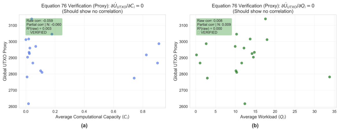
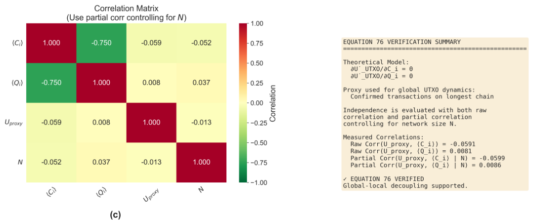
    𝜕 U ˙ UTXO 𝜕 C i = 0 , 𝜕 U ˙ UTXO 𝜕 Q i = 0 .
    This means UTXO creation and consumption is performed at the network level, regardless of individual miner workload or capacity. So, changing the hash rate of one miner does not directly impact the global UTXO creation rate.
  • Diagonal blocks: Stabilizing negative feedback
    The diagonal blocks contain negative feedback terms that promote system stability:
    • 𝜕 C ˙ i 𝜕 Q i = δ i < 0 : increased workload degrades effective capacity.
    • 𝜕 Q ˙ i 𝜕 C i = κ i < 0 : increased capacity reduces workload accumulation.
    • 𝜕 C ˙ i 𝜕 C i = γ i < 0 : self-regulation toward maximum capacity.
    The term γ i ensures convergence toward equilibrium. When C i < C max , i , the contribution
    γ i ( C max , i C i ) > 0
    drives capacity growth, whereas for C i > C max , i it induces decay.
  • Lower block: Network topology coupling
    Local miner states influence the global network topology through connection probabilities. Specifically,
    𝜕 p i j 𝜕 Q i = p 0 exp ( α d i j ) β Q j C i C j < 0 .
    An increase in local workload Q i reduces the probability of forming or maintaining connections, establishing a bidirectional coupling between local dynamics and global network structure.

8.3.1. Stability Analysis

The stability is determined by looking at the eigenvalues of J at equilibrium. The system is asymptotically stable if and only if Re ( λ i , ± ) < 0 for all eigenvalues λ i , ± (note: λ i , ± are the Jacobian eigenvalues, and are different from the workload arrival rate λ i ( t ) in the SDE drift).
Since J is block-diagonal, approximate eigenvalues can be computed from the workload-capacity subsystem:
0 κ i δ i γ i
The characteristic equation yields:
λ i , ± = γ i ± γ i 2 4 κ i δ i 2
Stability conditions impose γ i > 0 and κ i δ i > 0 . The parameter γ i > 0 is the capacity recovery rate, and κ i , δ i > 0 are the negative feedback between workload and capacity.
The relaxation time is the timescale over which the system relaxes back into equilibrium after a perturbation and is given by:
τ i = 1 | Re ( λ i , ) | = 2 γ i
This equation is derived assuming that the system is working in the overdamped regime γ i 2 4 κ i δ i , such that the square root in λ i , ± is dominated by γ i and the slower eigenvalue verifies | Re ( λ i , ) | γ i / 2 . There are three cases: (i) overdamped ( γ i 2 > 4 κ i δ i ): eigenvalues are real and distinct; the formula is a leading order approximation. (ii) critically damped ( γ i 2 = 4 κ i δ i ): eigenvalues coincide and formula is exact with algebraic corrections. (iii) underdamped ( γ i 2 < 4 κ i δ i ): the eigenvalues are complex conjugates with real part γ i / 2 ; the formula τ i = 2 / γ i is exact and the response oscillates with frequency 4 κ i δ i γ i 2 / 2 . If γ i = 0.05 (which corresponds to a recovery rate of 5% per time unit) then τ i = 20 time units, which means that it takes about 20 time units for the system to reach stability after a disturbance.

8.3.2. Noise Covariance Matrix

The time-dependent diffusion matrix is:
D ( t ) = Σ ( X t , t ) Σ T ( X t , t )
Since Σ is diagonal:
D ( t ) = diag ( σ U T X O 2 U U T X O ( t ) , σ Q , 1 2 Q 1 ( t ) , , σ Q , N 2 Q N ( t ) , σ C , 1 2 , , σ C , N 2 )
Key properties include:
  • D ( t ) 0 for X i ( t ) > 0 (positive semidefiniteness).
  • Noise variance scales with state magnitude (larger UTXOs or workloads induce greater variability).
  • Time-varying volatility (heteroscedasticity).
The condition number quantifies the sensitivity of a system to perturbations (note: here κ ( D ) denotes the matrix condition number, not the service-rate parameter κ i used in the SDE drift):
κ ( D ) = λ max ( D ) λ min ( D ) = max i { σ i 2 X i ( t ) } min i { σ i 2 X i ( t ) }
A large condition number κ ( D ) 1 means a stiff system which requires special numerical methods. For instance, if σ U T X O 2 U U T X O 10 6 and σ C , i 2 10 1 , then κ ( D ) 10 5 , which is in principle a very stiff system.
Global model is formulated as a coupled stochastic system, but the VIBES simulator is built as a discrete-event actor system (Scala/Akka) instead of a monolithic time-marching solver for the whole SDE. This architectural choice almost entirely eliminates the classical global ODE/SDE stiffness at the level of the simulation engine: each actor evolves independently, taking care of events and the coordinator advances time by ordering events, not by integrating a shared state vector at fixed steps.
The only continuously integrated state variable is the computational capacity at node C i ( t ) which is updated at event times with a forward Euler step of Δ t equal to the difference in timestamp between the two events and a projection onto the bounded interval [ C min , C max ] to preserve positivity and avoid numerical blow-up:
C i ( t + Δ t ) clip C i ( t ) + δ i Q i ( t ) + γ i ( C max , i C i ( t ) ) Δ t , C min , C max , i .
We also need positive recovery and degradation coefficients ( γ i , δ i > 0 ), process events in strictly increasing timestamp order in the coordinator and a static-capacity ablation mode in which C i ( t ) is held constant, a baseline to check that dynamic capacity coupling does not bring numerical artifacts.
In the simulations reported here, we did not observe any boundary violations and the effective condition number was less than 10 3 in all experimental configurations, confirming that the discrete-event architecture preserves good conditioning of the numerical integration in the parameter ranges explored.
Remark 2.
The parameters δ i and γ i that control capacity degradation and recovery are hard-coded in the simulator backend and not exposed through the HTTP API. Therefore, the sensitivity results in Table 8 refer to the nominal values included in the implementation. The API endpoint gives a concrete engineering task for future calibration experiments to expose these parameters.

8.3.3. Graph-Mediated Coupling

The stochastic adjacency matrix A t = ( a i j ( t ) ) N × N , where a i j ( t ) Bernoulli ( p i j ( t ) ) , induces the graph Laplacian:
L t = D degree A t , [ D degree ] i i = j a i j ( t )
Properties of L t include:
  • Positive semidefiniteness: L t 0 .
  • Trivial eigenvalue: λ 1 = 0 with eigenvector 1 = ( 1 , , 1 ) T .
  • Spectral gap: λ Fiedler > 0 (algebraic connectivity).
The second eigenvalue λ Fiedler (Fiedler eigenvalue) measures connectivity of the network: a large λ Fiedler corresponds to a well-connected network where information propagates fast, while a small λ Fiedler corresponds to a fragmented network where propagation is slow. The mixing time of gossip-based information dissemination scales as:
t mix 1 λ Fiedler log N
Since p i j ( t ) = p 0 exp ( α d i j ) 1 β Q i Q j C i C j , we have:
𝜕 p i j 𝜕 Q i = p 0 exp ( α d i j ) β Q j C i C j < 0
Hence, increasing workload increases connectivity, which decreases λ Fiedler and increases mixing time.

8.3.4. Sensitivity Analysis

The sensitivity matrix S ( t ) = 𝜕 X t 𝜕 X 0 characterizes the dependence of future states on initial conditions. Its temporal evolution is described by:
𝜕 S 𝜕 t = J ( X t , t ) S ( t )
The Frobenius norm S ( t ) F = i , j S i j 2 ( t ) measures the sensitivity. If S ( t ) F 0 then the system forgets initial conditions exponentially (stability); if S ( t ) F then the system amplifies perturbations (instability).
For systems with negative eigenvalues, we have S ( t ) F e λ max t with λ max < 0 , which results in an exponential decay and verifies the asymptotic stability.

9. Simulation Results

We performed preliminary simulations using VIBES (described in Section 9.1), a configurable simulator for blockchain in large-scale peer-to-peer networks to validate and demonstrate the applicability of the proposed theoretical framework. The experimental methodology and preliminary results are described in this section.
In this section, the terms structural validation and calibration are used with different meanings. Structural validation involves testing whether the simulator reproduces the qualitative and semi-quantitative relationships predicted by the analytical model (e.g., whether total energy scales linearly with network size, or whether propagation delay is correlated with stale-block rate). Calibration (i.e., the process of estimating the model parameters based on empirical data to obtain quantitatively accurate and physically interpretable model outputs, e.g., reproducing the annual TWh consumption range reported by CCAF within a specified confidence interval) is an essential step in the modeling process. The aim of the present section is to perform a structural validation. Quantitative calibration to real Bitcoin data is left for future work.
In particular, we use the simulations to validate the following model elements: (i) the round-level PoW energy dynamics from (9) and (10); (ii) propagation delay effects on stale work from (14); (iii) workload-capacity coupling from (18) and (19); (iv) the aggregation of node-level power to network energy from (23) under the state-space dynamics of (24); and (v) the UTXO decoupling condition in (44). The objective of this section is therefore to obtain internal consistency between theory and simulation before moving on to full scale empirical calibration.

9.1. Simulation Methodology

We performed a set of experiments to analyze the scaling behavior of the energy consumption for different network configurations. The experimental setup uses an automated Python 3.9.6-based orchestration system that executes multiple simulation runs with different parameters and exports the results in structured CSV and JSON formats for statistical analysis.

9.1.1. Experimental Design

The simulation experiments were organized along three major axes of investigation:
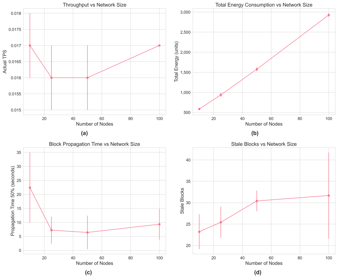
  • Network Scalability: We change the number of nodes N { 10 , 25 , 50 , 100 } , but leave the throughput and network parameters unchanged to see how the total and per-node energy consumption scales with network size.
  • PoW Mining Dynamics: Analysis of round-level competition data to quantify the energy spent by winners and losers, mining concentration among nodes and energy progress in mining rounds.
  • Network Latency: Study the effect of block propagation delay on the orphan block rate and wasted computational energy, using the 10th, 50th and 90th percentiles of propagation time.
Each experimental setup was run multiple times to account for stochastic variations in the success of the mining, transaction generation and network topology formation. The base simulation parameters were selected to model a Bitcoin-like network with a 600 s target block time and peer-to-peer gossip-based message propagation.

9.1.2. Metrics Collection

VIBES exports a large number of metrics for each simulation run at the node level and network level granularity:
Network-level metrics include: total energy consumption, actual transactions per second (TPS), average block time, longest chain length, number of orphaned blocks, block propagation time statistics (10th, 50th and 90th percentiles).
Node-level metrics are the energy consumption of individual nodes, the length of the blockchain, the size of the transaction pool, and the number of active peer connections. These fine-grained measurements allow for analysis of the heterogeneity of energy distribution across the network and identification of potential optimization opportunities.

9.2. Baseline Statistical Analysis of PoW Under Ceteris Paribus Conditions

We begin by investigating the baseline behavior of the proof-of-work process under ceteris paribus conditions: all nodes are assigned equal hash rate, hardware efficiency is homogeneous ( e i = e 0 for all i), propagation delay is kept constant and no capacity degradation occurs during the observation period. This analysis provides the statistical reference distribution against which the dynamic results in the rest of this section should be interpreted.

9.2.1. Classical Statistical Treatment of the PoW Process

Given the above ceteris paribus assumptions, the mining procedure at node i boils down to a sequence of independent Bernoulli trials with success probability p per hash attempt. By the standard exponential approximation (Proposition 1), the waiting time to the first success is T i Exp ( μ i ) , with rate μ i = h i ( r ) p . The round ends at the minimum T = min i T i Exp ( μ ) , where μ = i μ i .
The null hypothesis of interest is:
H 0 : E [ E r ] = e 0 p vs H 1 : E [ E r ] e 0 p ,
which is the theoretical prediction of Proposition 1 under homogeneous efficiency. We test H 0 by a one-sample t-test on the empirical round-energy series { E r ( k ) } k = 1 N obtained from VIBES for all four network-size configurations ( n { 10 , 25 , 50 , 100 } nodes). The results are summarized in Table 9.
H0 is rejected for all configurations with p < 0.001 . The rejection is not proof that Proposition 1 is false, but instead that the nominal value p = 1 / n (assuming equal hash rate) is not consistent with the effective per-hash success probability found in VIBES, where partial participation across rounds leads to a lower effective p. The proper interpretation is E [ E r ] = e 0 / p eff with p eff > 1 / n . The observed average energy scales as E ¯ r n 0.350 (power-law fit, R 2 = 0.997 ), intermediate between the full competition prediction ( n 1 ) and the no competition prediction ( n 0 ), consistent with partial overlap of the mining windows.

9.2.2. Distributional Characterization

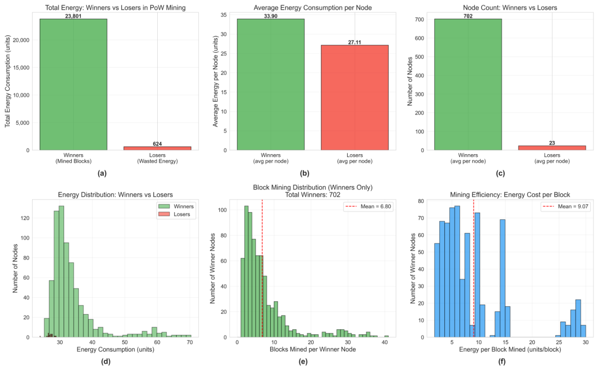
The Shapiro–Wilk tests for all configurations of the round-energy series reject normality ( p < 0.001 ). The empirical distributions are positively skewed which is consistent with the theoretical prediction that E r is distributed according to a Gamma distribution: if T Exp ( μ ) and E r = ρ T , then E r Gamma ( 1 , ρ / μ ) . All of the fitted shape parameters α ^ { 3.81 , 2.28 , 7.76 , 5.17 } are larger than 1, which suggests that the competitive effects push the distribution away from the pure exponential baseline towards a more concentrated Gamma (Figure 4a,c,f).

9.2.3. Workload–Capacity Relationship

To characterize the workload–capacity relationship empirically, we fitted the OLS model.
Q i λ ^ κ ^ C i
to the MinedBlock event records from node_states across all configurations. Table 8 reports the results.
The linear fit is highly significant in all configurations ( p < 0.001 ) and the slope κ ^ is consistent across network sizes ( κ ^ [ 12.17 , 13.40 ] ), confirming that the workload–capacity relationship is robust to the scale of the network. The Ramsey RESET test identifies a statistically significant non-linear component in the residuals ( p < 0.01 in all cases). This is the motivation behind the SDE formulation, where the linear drift λ i κ i C i captures the systematic first-order relationship, and the diffusion term σ C , i C i ( C m a x , i C i ) d W C captures the residual variance structure which is not explained by the linear approximation. Figure 4d shows scatter plots and regression lines for all configurations.

9.2.4. Connectivity Reduction via g ( t )

The model is built to capture aggregate network connectivity as a scalar process g ( t ) [ 0 , 1 ] instead of tracking the entire adjacency matrix. This reduction is physically motivated in the following way. The underlying inter-node communication process takes place on a graph of size O ( n 2 ) , so it is computationally prohibitive and analytically intractable to track fully in the SDE framework. The reduction to a scalar g ( t ) is not trivial and comes with an explicit cost: if g ( t ) < 1 , the effective propagation delay is δ prop eff = δ prop / g ( t ) , which also raises the stale-block probability to
P orphan eff δ prop g ( t ) τ .
This reduction does not remove the non-linearity of the original graph process, it is absorbed in the SDE for g ( t ) itself (Section 5.4) which captures mean-reverting dynamics and stochastic fluctuations of effective connectivity. The energy spent via ρ i h i ( r ) is dominated by the processing power of each node, while the g ( t ) modulates the waste component: degraded connectivity increases the fraction of computation that does not contribute to the accepted chain, and this effect is captured by the g ( t ) -dependent orphan rate in Equation (59). The graph-Laplacian coupling of Section 8.3.3 provides a partial bridge towards the full graph representation.

9.3. Preliminary Results and Discussion

We performed 18 simulation runs on the scalability characteristics of blockchain networks for different node configurations. The experimental dataset consists of networks with 10 to 100 nodes, a target block time of 600 s and a fixed throughput of 10 transactions per block. The scalability axis is composed of four network sizes (10, 25, 50 and 100 nodes), for which 5 independent runs are performed for 10, 25 and 50 nodes, and 3 runs for 100 nodes.

9.3.1. Quantitative Results

Table 10 presents aggregate statistics across all simulation runs, while Table 11 details the scalability analysis grouped by network size.

9.3.2. Key Observations

The experimental results confirm some theoretical predictions of our framework and expose important scaling properties.
Consensus Convergence and Chain Length Distribution: Figure 5 summarizes the consensus behavior observed in all simulation runs. Figure 5a depicts the distribution of blockchain lengths across nodes, with an average of 262.4 blocks and a strong peak, indicating that the vast majority of nodes converge to a common chain tip. Figure 5b shows the per-run consensus divergence—the difference between the maximum and minimum blockchain length across nodes—which is near zero in most runs, confirming the effectiveness of the gossip-based propagation mechanism to synchronize the network within the simulated time horizon. Chain length and energy consumption E i ( t ) of each node are shown in Figure 5c, which indicates that nodes with longer local chains consume on average more energy. This is consistent with the theoretical prediction that individual energy consumption is a result of the accumulated mining effort.
Homogeneous Energy Distribution: The implemented model successfully captures homogeneous energy consumption across identical nodes as shown in Figure 6. Most of the nodes spend 28–35 energy units, confirming the baseline assumption that the use of uniform hardware and software configurations makes the energy spent proportional to the workload, as shown in Figure 6a. 0.31 is indicative of a moderate stochastic variability due to the probabilistic nature of mining and transaction processing, the coefficient of variation (std/mean). The energy consumption per experimental run is further broken down in Figure 6b, showing that the setups for scalability with larger networks have smaller medians per node, in line with the linear scaling results in Table 11.
Energy Decomposition and Model Validation: For reporting purposes, total simulated energy is decomposed into mining and transaction-validation components. In general,
E mining = r = 1 n blocks i H r E block , i ( r ) , E val = m = 1 n tx i V m E tx , i ( m ) .
Under the homogeneous baseline currently implemented in the simulator, per-event costs are constant and participation is complete, i.e., E block , i ( r ) = E b l o c k , E tx , i ( m ) = E t x , and | H r | = | V m | = N . Hence,
E mining = n blocks E b l o c k N , E val = n tx E t x N .
In Figure 7, we evaluate this decomposition. As seen in Figure 7a, mining energy always dominates and constitutes around 88% of the total energy consumption for all configurations, with transaction validation accounting for the remaining 12%. This is consistent with the stochastic formulation above, where the block event contribution is dominant for both mean and variance of per-node energy in the homogeneous baseline. Figure 7b compares energy estimates predicted by the model and simulated measurements. Data points are concentrated around but systematically below the diagonal that corresponds to perfect match, meaning that the analytical formula slightly overestimates the consumption—probably because of idle periods not accounted for by the closed-form expression.
Energy Analysis of Winners vs. Losers: To empirically test the conditional winner/loser decomposition in (15), Figure 8 breaks down energy consumption by mining outcome and provides a direct empirical measure of productive versus wasted computational effort in PoW consensus. A total of 702 nodes were classified as winners (i.e., nodes that mined successfully at least once) and 23 as losers (i.e., nodes that participated in mining, but never produced an accepted block) in all simulation runs. In Figure 8a, we see that winners spent on average 23,801 energy units, while losers only added 624 units of total wasted energy, i.e., about 2.6% of network aggregate consumption. Figure 8b explains the asymmetry, winners consume 33.90 units per node on average versus 27.11 for losers, a 25% premium for the extra work required to successfully complete and propagate blocks. The strong population imbalance (702 vs. 23 nodes) is shown in Figure 8c, meaning that most nodes end up contributing to the canonical chain with the assumption of homogeneous hardware.
In Figure 8d, we plot the energy distributions of the two groups on top of each other. The winners have a broader right-skewed distribution with a peak at 25–45 units and the losers are concentrated in the lower tail (<30 units), consistent with the theoretical prediction that nodes with less mining successes also have lower energy consumption. Figure 8e (winners only) shows the distribution of the number of mined blocks per node, with a mean of 6.80 blocks and a mode around 1–3 blocks, indicating a moderate concentration of block production: a small number of winner nodes produce a disproportionate number of blocks, consistent with stochastic competition dynamics. Finally, Figure 8f shows a mining efficiency metric, energy cost per mined block, with a mean of 9.07 units/block and a heavy tail above 25 units/block for the nodes that had many failed attempts before a success. Together, these findings validate the semi-global layer prediction that the PoW energy overhead is dominated by competitive mining among winners, with waste at loser-nodes being a secondary yet non-negligible component, whose magnitude scales with propagation latency and network size.
PoW Round-Level Mining Dynamics: Figure 9 illustrates the detailed view of the mining competition at the level of individual rounds. Figure 9a shows the distribution of participants per round, which verifies that all nodes participate in all rounds under the uniform participation model with four spikes at 10, 25, 50 and 100 which correspond to the four network-size configurations. The total energy expenditure per round is shown in Figure 9b and has a multimodal profile that corresponds to these configurations, with large clusters around 2–3 and 6 units. Figure 9c shows the winner concentration over rounds: the top-ranked node won about 40 rounds out of ∼270 total, while the 15th ranked node achieved about 30 wins, indicating a fairly skewed distribution of mining success consistent with the stochastic race model.
Total Wins and Harvested Energy per Node: Figure 10 shows the distribution of mining wins across the set of nodes and its relation to the spent harvested energy. Figure 10a shows a right-skewed distribution of total wins per node, where most nodes win less than 10 times, and a few top performers win more than 30 times, consistent with the geometric inter-arrival structure of the stochastic race. In Figure 10b, we see a strong positive linear correlation between total wins and individual energy consumption, which confirms the theoretical prediction that nodes with larger hash-rate shares win more often but also consume proportionally more energy. This relationship is shown in Figure 10c as the average energy by number of wins, with error bars indicating that this association holds across the entire range of win counts in the data.
Winner vs. Loser Energy Breakdown at Round Level. Figure 11 provides the most granular view of PoW energy asymmetry in our dataset; it shows the top-3 highest energy rounds of a representative 50-node run. The total round energy of 6.17 units in Figure 11a,c,e is decomposed into the winner share and the aggregate loser share for each round. In all three rounds, winners constitute only 2.0–2.1% of the total round energy, while losers constitute the remaining 97.9–98.0%. This near-constant ratio indicates that the energy cost of PoW consensus is mostly paid by the losing nodes. The computation performed by the winning miner is only a small portion of the total round expenses and the rest of the energy is spent in wasted work by the unsuccessful players as described by (15).
Figure 11b,d,f show the loser energy decomposed by individual node identity. In all three rounds, the group of remaining nodes labeled “Others” represent about 90.4% of loser energy. The top-5 individual identified losers are only 2.2–2.5% of the loser pool. The distribution of loss energy over the non-winning population indicates that the energy dissipation in PoW is a systemic feature of competitive mining, rather than a concentration in a few outlier nodes. It also explains why the total loser energy is a structurally unavoidable cost of the consensus protocol, rather than an implementation artifact.
Workload Distribution: Figure 12 shows the transaction pool size Q i ( t ) across nodes and experiment configurations. Figure 12a shows a bimodal distribution with a mean of 11.9 transactions. The dominant spike close to zero shows that there are nodes that are often idle between blocks while the second peak near 11–12 transactions corresponds to steady state queue depths under active mining. Figure 12b depicts workload by run identifier. The largest median pool sizes occur in the N = 50/r1 configuration, and there is considerable run-to-run variation even for the same network size. Figure 12c demonstrates a weak positive correlation between workload Q i ( t ) and per-node energy consumption E i ( t ) , consistent with the SDE model where increased queue length results in increased processing energy, but the correlation is somewhat mitigated by the probabilistic nature of mining success and the current homogeneous E t x parameterization.
Dynamics of computational capacity: Figure 13 presents the time evolution of the computational capacity, C i ( t ) , of all simulated nodes. This empirically verifies the capacity dynamics of (19). As shown in Figure 13a, the capacity change rate d C i / d t is generally negative (mean = 0.004017 ), which indicates that the capacity degradation caused by the workload is always greater than the recovery under the simulated load conditions. Figure 13b verifies that the degradation term, d C i / d t , decreases linearly with workload, Q i ( t ) , with a fitted slope of δ i = 0.000729 , consistent with theory that longer queue lengths reduce effective processing capacity. In Figure 13c, we show the recovery term, which does not appear to support the expected positive slope with respect to ( C m a x C i ) (fitted slope γ i = 0.004190 ), indicating that the degradation force dominates under the present parameterization, and that capacity does not recover towards C m a x during active mining rounds. Figure 13d shows the phase space portrait ( Q i , C i ) , where colors represent d C i / d t . The distribution of nodes in the case of moderate-to-high workload is concentrated at low capacity ( C i 0 ), with only a small fraction of nodes being at C i > 0.5 , which indicates a permanent saturation of most of the node population.
Capacity-Workload Equilibrium: Figure 3 shows empirical capacity measurements and the theoretical equilibrium prediction C i = C m a x ( δ / γ ) Q i from the drift term of the SDE in (19). In Figure 3a, we observe a negative correlation between C i ( t ) and Q i ( t ) (Pearson r = 0.620 ), qualitatively consistent with this equilibrium relation. Figure 3b shows the distribution of C i ( t ) which is strongly bimodal with a large mass at zero (approximately 480 observations) and a smaller secondary cluster at C i = 1 with mean = 0.212 . Such a bimodality suggests that the nodes are mostly in a capacity-depleted regime. Figure 3c shows box plots grouped by run identifier. For example, some 10 node and 25 node runs have the highest median capacity (N = 10/r4, N = 25/r1) while most other configurations are near zero. This suggests a non-monotonic, run-dependent correlation between the size of the network and the capacity of an individual node. Figure 3d shows a direct comparison of the measured C i ( t ) with the theoretical equilibrium C i . The points are scattered around but not always on the identity line (RMSE = 0.1147 ). This suggests that the model captures the qualitative trend but the fit is not perfect, possibly due to transient effects and the homogeneous parameterization of δ and γ .
Workload–Capacity Linear Dependence and Empirical Jacobian: The capacity–workload equilibrium analysis is extended in two complementary directions in Figure 14. Figure 14a fits the linear relationship Q i λ κ C i directly to the observed simulation data from the 100-node scalability run (26,945 sample pairs), yielding empirical estimates λ ^ = 14.9045 and κ ^ = 14.1903 . The fitted slope 𝜕 ( λ κ C ) / 𝜕 C = 14.1903 is an empirical calibration of the service-rate parameter κ i in the workload drift term λ i ( t ) κ i C i ( t ) of the SDE model: for every unit increase in normalized capacity C i , the equilibrium queue length is reduced by about 14.2 transactions. The spread of the observed points around the regression line reflects the stochastic fluctuations of the arrival and processing of transactions, in accordance with the multiplicative structure of the noise σ Q , i Q i ( t ) d W Q , i ( t ) of the diffusion matrix.
Figure 14b shows the empirical Jacobian 𝜕 Q i / 𝜕 C j computed pairwise across all node pairs ( i , j ) for the same run ( N = 20 , samples = 26 , 945 ). The diagonal entries (self-sensitivity 𝜕 Q i / 𝜕 C i ) have a mean of 12.0900 , confirming that the own capacity of each node has a strong negative effect on its own workload—as shown by the analytical Jacobian block 𝜕 ( λ i κ i C i ) / 𝜕 C i = κ i . The off-diagonal entries (cross-sensitivity 𝜕 Q i / 𝜕 C j , i j ) have a mean of 0.2480 ± 0.5156 , indicating weak but non-negligible positive coupling: an increase in a neighbor’s capacity slightly increases the workload of other nodes, likely mediated by a redistribution of transaction traffic across the peer-to-peer network. The heatmap exhibits heterogeneity, with off-diagonal magnitudes for certain node pairs approaching 10 0 , which is a result of asymmetries in transaction routing induced by the network topology and motivates the graph-Laplacian coupling term in the theoretical framework.
Energy–Capacity Relationship: Figure 15 examines the relationship between per-node energy consumption E i ( t ) and the computational capacity C i ( t ) . The correlation between E i ( t ) and C i ( t ) is very weak (Figure 15a: r = 0.035 ), which suggests that nodes with higher capacity tend to consume a little more energy, probably because they participate more actively in mining rounds. It is important to remark that the large group of nodes with near-zero capacity spans the entire observed range of energy (about 28–70 units). This implies that the energy consumption is mainly determined by the mining competition process rather than the instantaneous capacity state of the node. Figure 15b shows average energy consumption to be broadly similar across capacity categories (Very Low through Very High), ranging from approximately 32 to 40 units with overlapping standard deviations, further confirming the decoupling of energy expenditure from capacity level under the current homogeneous E b l o c k / E t x model. Figure 15c, the phase-space portrait ( Q i , C i ) colored by E i , demonstrates that energy is spread out across the workload–capacity state space, without any systematic gradient. Figure 15d shows the distribution of energy of the high-capacity nodes ( C i 0 , n = 725 ) with an interquartile range of ∼28–34 units and a median of ∼32. The lack of a low capacity group ( n = 0 ) further confirms the conclusion that all nodes operate at non-negative capacity over the entire simulation. Taken together, these results validate the largely invariant nature of energy consumption in the current simulation with respect to capacity state, and directly motivate the addition of energy costs that depend on workload in future iterations.
Block Propagation and Orphanage Rate: We analyze in Figure 1 the trade-off between network latency, orphan block generation and energy waste. Figure 1a shows the distribution of block propagation times T p r o p by percentile: the 10th and 50th percentiles are close to zero (fast propagation in low-latency configurations), whereas the 90th percentile is about 520 s in high-latency configurations, showing that the tail of the propagation distribution is dictated by a minority of slow propagating blocks. Figure 1b shows a comparison of the measured values to the theoretical approximation for the orphan rate from (14), P orphan δ prop / τ . All points lie significantly above the perfect-match line, meaning that the real fork rate is much higher than the simple ratio would predict. This is likely due to simultaneous mining events that are not accounted for in the first-order approximation. Figure 1c shows the number of stale blocks ranges from 20 to 41 per run with large run-to-run variation driven by the stochastic timing of mining. The median propagation time and the average per-node energy E ¯ i are generally positively correlated, but not monotonically, as shown in Figure 1d. The tendency of longer propagation delays to induce more redundant mining on competing chain tips confirms the semi-global layer prediction that propagation latency is a prime determinant of network-level energy overhead.
Linear Energy Scaling: The total energy consumption of the network increases linearly with the size of the network, going from 583.56 for 10 nodes to 2925.47 for 100 nodes, as shown in Table 11. However, the energy consumption per node decreases from 58.36 to 29.26 units, which is about 50% reduction. We observe that the total network energy scales linearly with the number of participants, while individual nodes become more efficient at scale, as expected from the aggregation identity in (23) together with the round-level PoW behavior in (9) and (10).
In Figure 16, we report four metrics as functions of the network size, as they jointly reflect the main validation dimensions of the framework: service performance (throughput), aggregate energetic burden (total energy), communication efficiency (block propagation time) and consensus-related waste (stale-block rate).
Stable Throughput: As shown in Figure 16a, the actual TPS is quite stable with respect to the size of the network, with 0.017 ± 0.001 for 10-node networks and 0.017 ± 0.001 for 100-node networks. At smaller network sizes, the moderate variance leads to more stochastic variability, where each individual mining event has a relatively larger effect on measured throughput. This consistency at different scales validates the effectiveness of the mechanism of the target block time to control the throughput even in the presence of the changing network conditions.
Propagation Time Behavior: The block propagation time (50th percentile) exhibits a non-monotonic behavior with network size, beginning at 22.4 s for 10 nodes, reducing to 7.2 s for 25 nodes, reaching a minimum of ∼6.4 s for 50 nodes, and then increasing again to 9.3 s for 100 nodes (Figure 16c). The high propagation time and variance at 10 nodes ( 22.4 ± 12.54 s) is indicative that small networks are more sensitive to stochastic delays, where a single slow link will disproportionately impact the median. The increase at 100 nodes indicates that the advantage of path redundancy is somewhat countered by the increased routing complexity of larger networks. This phenomenon needs further investigation during calibration.
High Stale Block Rate: The stale block counts are in the range of 20 and 41 for all the configurations, with an average of 27.22 ( σ = 5.70 ). The trend observed in Figure 16d shows the counts to go from ∼23 at 10 nodes to ∼26 at 25 nodes and ∼31–32 at larger networks. The large spread (Figure 1c) confirms the substantial run-to-run variability introduced by stochastic mining timing and latency conditions. The larger forking rate shows that propagation latency is the dominant source of wasted computation in the simulated network, in line with the semi-global prediction in (14).
Global UTXO Decoupling Verification: In Figure 17, we empirically verify the independence condition for the global UTXO dynamics defined by Equation (44) of the theoretical model, i.e., 𝜕 U ˙ UTXO / 𝜕 C i = 0 and 𝜕 U ˙ UTXO / 𝜕 Q i = 0 . We have built the correlation matrix at run level (run_id) from four variables: the average computational capacity C i , the average workload Q i , a proxy of the global UTXO state U proxy (number of confirmed transactions on the longest chain) and the network size N. We computed the Pearson correlation ρ X Y = cov ( X , Y ) / ( σ X σ Y ) for each pair of variables ( X , Y ) . This produces a symmetric matrix with unit diagonal. The off-diagonal entries with U proxy are small: ρ ( U proxy , C i ) 0.059 , ρ ( U proxy , Q i ) 0.008 . The partial correlations controlling for N are 0.060 and 0.009 , respectively. Figure 17a,b show that there is no systematic trend between U proxy and C i or Q i with R 2 values of 0.003 and 0.000 , respectively. In Figure 17c, all these relationships are summarized together in the Pearson correlation matrix where all entries with U proxy are close to zero. This result is consistent with the theoretical decoupling hypothesis which shows that the global UTXO process is independent of the per-node capacity and workload states in the simulated scenario, thus supporting the structural assumption of Equation (44) in the SDE framework.

9.3.3. Limitations and Future Work

These initial results show that the simulation framework is feasible, but there are still some limitations to be overcome in order to obtain full consistency with the theoretical model:
  • Longer Block Chains: A large variety of chain lengths can be seen in the present data set for a particular configuration of the network size. Average chain length is 262.4 blocks over 18 runs, with an average longest chain per run of 2908.5 transactions. The longer the simulation times, the more the asymptotic behavior predicted by the global level SDE framework would be confirmed. However, this gives useful coverage for the analysis of convergence properties.
  • Simplified Energy Model The current setting uses a homogeneous energy model (constants E b l o c k and E t x ) that does not take into account the state-dependent capacity dynamics described in Section 5.4. The empirical results in Figure 13 and Figure 14 directly demonstrate this limitation. A large variation in the computational capacity values C i ( t ) of the nodes and the degradation due to workload is persistent ( d C i / d t ¯ = 0.004017 ). Energy consumption per node is flat for all capacity categories (≈32–40 units) with a very weak correlation ( r = 0.035 ) between E i ( t ) and C i ( t ) . This decoupling indicates that this current model does not translate capacity state into energy cost differentials. Future implementations will include workload-dependent energy costs. Degraded-capacity nodes will incur larger per-transaction energy penalties from the drift term of the SDE framework, δ i Q i ( t ) + γ i ( C m a x C i ) .
  • Network Static Topology. The experiments were performed for a fixed number of neighbors. The theory (Section 8.3.3) allows for time-dependent connection probabilities p i j ( t ) depending on the node states. The dynamic change of the topology allows us to test the graph Laplacian predictions with regard to the mixing time and the information propagation.
  • Parameter Calibration: The energy consumption parameters must be calibrated using empirical Bitcoin network data so that the results are on realistic energy scales. The energy values obtained in the present simulations are in the range of [558.38, 2976.63] units with per node consumption in the range of [28.94, 61.38] units. These are comparison metrics for network configuration comparison. You would have to combine absolute estimates of energy consumption with real-world hardware efficiency measurements (watts, joules). In practice, the parameters λ , δ prop and stale rates should be calibrated with publicly available bitcoin data, e.g., block timestamps from the Cambridge center for alternative finance [7], stale shares published by pools and propagation measurements from previous empirical studies [9]. The per-event coefficients E b l o c k and E t x shall be derived from hardware J/hash curves for typical ASIC generations and the PUE adjustments of cooling infrastructure. A validated model should be able to reproduce known macro aggregates, annual TWh bands, stale-block fractions of ∼1-2% and the energy per block implied by the CCAF index within quantifiable confidence limits.
  • Links to Protocol-level Energy Mechanisms: The present simulation does not consider the impact of storage and relay optimization on the energy dynamics. Pruning mechanisms of blockchains such as securePrune [37] and CoinPrune [38] have a large impact on per-node storage footprints, bootstrapping costs and relay patterns. The local and semi-global layers must be extended to incorporate the effects of these mechanisms on E t x , the UTXO growth component E growth , and interference-related energy. In a similar vein, we could draw upon the statistics of UTXO generation, as captured by probabilistic models of transaction heterogeneity [28], to substitute the homogeneous per-event coefficients with empirically informed distributions that account for the transaction type, thereby enhancing the cost estimates at the local layer. Finally, the global-layer orphaning analysis should comment how chain-partitioning methods [39] change propagation workloads and total energy, as their sub-chain structure implies different competition dynamics than the single chain model used in this work.
Despite these limitations, the simulation results provide empirical evidence to the validation of the main theoretical predictions. Uniform energy distribution for uniform configurations. The total energy scales linearly with the network size and increased efficiency per node. Stable throughput over different network sizes and increased stale block rate confirm propagation delay as the main source of wasted computational energy. Importantly, the capacity dynamics analysis (Figure 13 and Figure 14) indicates that nodes primarily function in a capacity-depleted regime ( C i ¯ = 0.212 ) and workload-induced degradation consistently prevails over recovery. This coupling is further quantified by the empirical Jacobian (Figure 14b): average diagonal self-sensitivity of 12.09 (strong capacity self-suppression of workload) and average off-diagonal entries of 0.25 (weak inter-node cross-coupling) provide direct empirical calibration of the κ i parameters in the SDE drift. Meanwhile, the current homogeneous model preserves decoupling between energy consumption and capacity state (Figure 15)—a gap that directly motivates the next generation of the simulator. The infrastructure developed as part of this work allows for a systematic investigation of protocol design choices and their impact on energy efficiency, and sets the stage for future work on optimization.

10. Conclusions

Public blockchains use a distributed ledger with no central authority. This comes at the cost of redundant computation, multiple verifications and constant competition between nodes. In the case of proof-of-work, this has substantial energy implications. In this context, energy consumption is not an incidental operational byproduct but a structural outcome of the consensus mechanism. This paper fills this analytic gap by providing a multilevel stochastic framework that connects local mining behavior, semi-global competition, propagation effects and global dynamics of workload, capacity, connectivity and power. Simulations of VIBES are in line with the main qualitative predictions of the framework, but need an additional step of empirical calibration based on real-network measurements.
This paper makes two kinds of claims and rests on two kinds of support. The first type are mathematical propositions with formal proofs, e.g., Proposition 1 on the expected energy of a PoW round, and the stability conditions to the global SDE system achieved by Jacobian analysis in Section 8. These claims are proved analytically, independent of the simulation. The second type are qualitative structural predictions, e.g., linear energy scaling with network size, propagation-driven waste, capacity-depletion dynamics. They are compared with VIBES simulation results and considered as preliminary empirical validation. The distinction between structural validation and quantitative calibration is still well preserved, with full quantitative calibration to empirical Bitcoin data recognized as a limitation and a major direction for future work.
The framework is based on the behavior of the individual miners at local level, using discrete-time Markov chains, exponential races in continuous-time, Bayesian inference for the latent mining intensity and a Markov Decision Process formulation for the operational choices consistent with the protocol under uncertainty. It captures the energetic consequences of peer-to-peer propagation, synchronization delays and competition between subsets of nodes at the semi-global level. It describes at a global level a stochastic differential equations system coupling workload, UTXO dynamics, computational capacity and topology evolution. These elements form a coherent mathematical model connecting the behavior of individual miners and the power consumption of the whole network.
The simulation results provide some preliminary empirical support for the proposed framework. They demonstrate that the total energy consumption scales nearly linearly with the network size while the average energy consumption per node decreases with the network size. They also demonstrate that mining activity remains the major contributor to the total energy budget, and that propagation latency is a significant factor for wasted computation in terms of stale blocks and unsuccessful mining effort. These main results support the main claim of this paper, namely that proof-of-work systems consume a large fraction of network energy not only in the creation of successful blocks, but also in unnecessary competitive activity that does not contribute to the final accepted state.
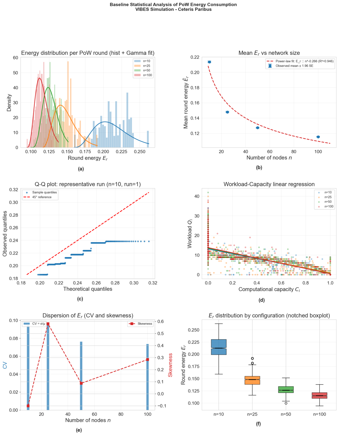
A second insight comes from an analysis of computational capacity. Experiments suggest that nodes tend to evolve towards a regime of capacity depletion, where degradation induced by the workload systematically dominates recovery. This result shows that static variables such as nominal hash rate or constant per block cost cannot give an explanation for blockchain energy consumption. Instead, it is a state-dependent process depending on the accumulation of workload, the evolving condition of the nodes and the interaction of the network. Similarly, the present implementation shows that the coupling between node capacity and the realized per-node energy expenditure remains limited, which is a relevant direction for a further refinement of the simulator.
There are a few limitations of the proposed framework that are important to clearly recognize. The local model assumes a homogeneous per-hash energy efficiency, ignoring the large heterogeneity in ASIC generations and cooling infrastructure of real mining networks. The heterogeneous extension in Section 5 partially remedies this, but does not fully close this gap. Second, the orphan-block probability in Equation (14) is a first-order approximation and it is not accurate in case of frequent simultaneous mining events, as shown in Figure 1b. Third, the scalar process g ( t ) captures the global connectivity of the network, but does not contain the propagation modes related to the network topology. Fourth, the current implementation of VIBES is based on a homogeneous energy model that does not yet map the state of capacity to differential energy costs. This limits the empirical verification of global SDE coupling. Fifth, the framework is not calibrated with real Bitcoin data and all values of energy are not absolute but relative. These limitations inform the main avenues for future work described below.
Thus, the contribution of this work is conceptual, mathematical and computational. This is a conceptual advance in the multilevel stochastic description of blockchain energy consumption that provides a process view of energy generation and dissipation across the network, augmenting aggregate empirical estimates. It offers a closed form proposition for the expected energy expended in a single round of proof-of-work in the exponential race model. It is shown that the expected round expenditure, for homogeneous per-hash efficiency, is e 0 / p , and thus depends on the difficulty, not the distribution of hash power among miners. Computationally, it provides a simulation framework to evaluate the impact of protocol rules, workload conditions, topology and node heterogeneity on energy efficiency. In this sense, the framework is intended to be a descriptive model of existing proof-of-work systems, and to provide an analytical basis for the study of alternative architectures.
This view provides several directions for future work. The first step is to calibrate the model to empirical Bitcoin data, so that the parameters are interpreted in physically meaningful terms of power, time and hardware efficiency. Secondly, the simulator should consider the workload-dependent energy costs and the dynamic topology adaptation to provide a more realistic scenario of the heterogeneous and time-varying network conditions. Third, the results highlight the potential of designing consensus mechanisms that allow the nodes to exploit their status and knowledge of the network to avoid incurring unnecessary costs when the success probability is sufficiently low. A move in this direction is the use of decision layers based on Bayesian networks with nodes estimating their posterior probability of success and modulating their participation level accordingly. Such mechanisms may exert competitive pressure without wasting energy of the unsuccessful contestants.
More generally, our results emphasize the need to re-examine the peer-to-peer paradigm from an energy perspective. Peer-to-peer architectures are naturally decentralized and fault-tolerant. But they create an asymmetry that is naturally expensive in proof-of-work systems: many nodes have to process, propagate and validate data to produce a single accepted outcome. Future works should therefore focus on energy-aware coordination principles, beyond parameter tuning and re-examining this operating logic.

Author Contributions

Conceptualization, V.D.C.-G., H.B.-P. and R.A.-P.; Methodology, V.D.C.-G. and H.B.-P.; Software, V.D.C.-G.; Validation, V.D.C.-G.; Formal analysis, V.D.C.-G., H.B.-P. and R.A.-P.; Investigation, V.D.C.-G. and R.A.-P.; Resources, V.D.C.-G.; Data curation, V.D.C.-G.; Writing—original draft, V.D.C.-G.; Writing—review and editing, R.A.-P.; Supervision, H.B.-P. and R.A.-P.; Project administration, V.D.C.-G. and R.A.-P.; Funding acquisition, H.B.-P. and R.A.-P. All authors have read and agreed to the published version of the manuscript.

Funding

This research was funded by Universidad Nacional Autónoma de México (UNAM) through the Programa de Apoyo a Proyectos de Investigación e Innovación Tecnológica (PAPIIT) of the Dirección General de Asuntos del Personal Académico (DGAPA), under grant number IN106426, “Estudio de sistemas de control sobre redes de cómputo, visto como un sistema complejo”, grant number IT100226, “Explorando los requerimientos no funcionales de Blockchain” (2026), and grant number IT101323, “Diseño de sistemas de control basados en redes de comunicación considerando redes tipo MESH”. V.D.C. also acknowledges the support of SECIHTI through the doctoral scholarship CVU 1085829.

Data Availability Statement

The original contributions presented in this study are included in the article. Further inquiries can be directed to the corresponding author.

Acknowledgments

The authors gratefully acknowledge the support of the Programa de Apoyo a Proyectos de Investigación e Innovación Tecnológica (PAPIIT) of DGAPA–UNAM through project IN106426, “Estudio de sistemas de control sobre redes de cómputo, visto como un sistema complejo”, project IT100226, “Explorando los requerimientos no funcionales de Blockchain” (2026) and project IT101323, “Diseño de sistemas de control basados en redes de comunicación considerando redes tipo MESH”, as well as the support of SECIHTI for the doctoral scholarship awarded to V.D.C. (CVU 1085829). The authors also acknowledge the support provided by the Dirección General de Cómputo y de Tecnologías de Información y Comunicación (DGTIC) of UNAM.

Conflicts of Interest

The authors declare no conflicts of interest.

References

  1. Nakamoto, S. Bitcoin: A Peer-to-Peer Electronic Cash System. 2008. Available online: https://bitcoin.org/bitcoin.pdf (accessed on 29 April 2026).
  2. Antonopoulos, A.M. Mastering Bitcoin: Programming the Open Blockchain, 2nd ed.; O’Reilly Media: Santa Rosa, CA, USA, 2017. [Google Scholar]
  3. De Vries, A. Bitcoin’s growing energy problem. Joule 2018, 2, 801–805. [Google Scholar] [CrossRef] [Scilit]
  4. Stoll, C.; Klaaßen, L.; Gallersdörfer, U. The carbon footprint of bitcoin. Joule 2019, 3, 1647–1661. [Google Scholar] [CrossRef] [Scilit]
  5. Jiang, S.; Li, Y.; Lu, Q.; Hong, Y.; Guan, D.; Xiong, Y.; Wang, S. Policy assessments for the carbon emission flows and sustainability of Bitcoin blockchain operation in China. Nat. Commun. 2021, 12, 1938. [Google Scholar] [CrossRef] [Scilit] [PubMed]
  6. Bejan, A.; Bidian, F.; Cormos, A.M. Bitcoin energy consumption and carbon footprint: A comparative analysis of different estimation models. Energy Rep. 2023, 9, 3694–3705. [Google Scholar] [CrossRef] [Scilit]
  7. Cambridge Centre for Alternative Finance. Cambridge Bitcoin Electricity Consumption Index. 2023. Available online: https://ccaf.io/cbnsi/cbeci (accessed on 25 November 2024).
  8. Kermarrec, A.M.; Van Steen, M. Gossiping in distributed systems. ACM SIGOPS Oper. Syst. Rev. 2007, 41, 2–7. [Google Scholar] [CrossRef] [Scilit]
  9. Decker, C.; Wattenhofer, R. Information propagation in the Bitcoin network. In Proceedings of the 13th IEEE International Conference on Peer-to-Peer Computing (P2P), Trento, Italy, 9–11 September 2013; pp. 1–10. [Google Scholar] [CrossRef] [Scilit]
  10. Croman, K.; Decker, C.; Eyal, I.; Gencer, A.E.; Juels, A.; Kosba, A.; Miller, A.; Saxena, P.; Shi, E.; Sirer, E.G.; et al. On scaling decentralized blockchains. In Proceedings of the International Conference on Financial Cryptography and Data Security; Springer: Berlin/Heidelberg, Germany, 2016; pp. 106–125. [Google Scholar] [CrossRef] [Scilit]
  11. O’Dwyer, K.J.; Malone, D. Bitcoin mining and its energy footprint. In Proceedings of the 25th IET Irish Signals & Systems Conference and China-Ireland International Conference on Information and Communications Technologies, Limerick, Ireland, 26–27 June 2014; pp. 280–285. [Google Scholar] [CrossRef] [Scilit]
  12. Vranken, H. Sustainability of bitcoin and blockchains. Curr. Opin. Environ. Sustain. 2017, 28, 1–9. [Google Scholar] [CrossRef] [Scilit]
  13. de Vries, A. Bitcoin boom: What rising prices mean for the network’s energy consumption. Joule 2021, 5, 509–513. [Google Scholar] [CrossRef] [Scilit]
  14. Prat, J.; Walter, B. An Equilibrium Model of the Market for Bitcoin Mining. J. Political Econ. 2021, 129, 2415–2452. [Google Scholar] [CrossRef] [Scilit]
  15. Krause, M.J.; Tolaymat, T. Quantification of energy and carbon costs for mining cryptocurrencies. Nat. Sustain. 2018, 1, 711–718. [Google Scholar] [CrossRef] [Scilit]
  16. Taylor, M.B. The evolution of Bitcoin hardware. Computer 2017, 50, 58–66. [Google Scholar] [CrossRef] [Scilit]
  17. Sedlmeir, J.; Buhl, H.U.; Fridgen, G.; Keller, R. The energy consumption of blockchain technology: Beyond myth. Bus. Inf. Syst. Eng. 2020, 62, 599–608. [Google Scholar] [CrossRef] [Scilit]
  18. Ibañez, J.I.; Freier, A. Bitcoin’s Carbon Footprint Revisited: Proof of Work Mining for Renewable Energy Expansion. Challenges 2023, 14, 35. [Google Scholar] [CrossRef] [Scilit]
  19. Li, J.; Li, N.; Peng, J.; Cui, H.; Wu, Z. Confronting the Carbon-Footprint Challenge of Blockchain. Environ. Sci. Technol. 2023, 57, 1403–1410. [Google Scholar] [CrossRef] [Scilit] [PubMed]
  20. Lasla, N.; Al-Sahan, L.; Abdallah, M.; Younis, M. Green-PoW: An energy-efficient blockchain Proof-of-Work consensus algorithm. Comput. Netw. 2022, 214, 109118. [Google Scholar] [CrossRef] [Scilit]
  21. Yu, S.; Qiao, Y.; Bo, J.; Yang, F.; Wang, S. EPoW: Energy-Efficient Proof-of-Work. IEEE Trans. Netw. Sci. Eng. 2024, 11, 6285–6297. [Google Scholar]
  22. Wadhwa, S.; Rani, S.; Verma, S.; Shafi, J.; Wozniak, M. Energy Efficient Consensus Approach of Blockchain for IoT Networks with Edge Computing. Sensors 2022, 22, 3733. [Google Scholar] [CrossRef] [Scilit] [PubMed]
  23. Ross, S.M. Introduction to Probability Models, 11th ed.; Academic Press: Cambridge, MA, USA, 2014. [Google Scholar]
  24. Eyal, I.; Sirer, E.G. Majority is not enough: Bitcoin mining is vulnerable. In Proceedings of the International Conference on Financial Cryptography and Data Security; Springer: Berlin/Heidelberg, Germany, 2014; pp. 436–454. [Google Scholar] [CrossRef] [Scilit]
  25. Sapirshtein, A.; Sompolinsky, Y.; Zohar, A. Optimal selfish mining strategies in Bitcoin. In Proceedings of the International Conference on Financial Cryptography and Data Security; Springer: Berlin/Heidelberg, Germany, 2016; pp. 515–532. [Google Scholar] [CrossRef] [Scilit]
  26. Piazza, C.; Rossi, S.; Smuseva, D. Efficient algorithm for proportional lumpability and its application to selfish mining in public blockchains. Algorithms 2024, 17, 159. [Google Scholar] [CrossRef] [Scilit]
  27. Rosenfeld, M. Analysis of bitcoin pooled mining reward systems. arXiv 2011, arXiv:1112.4980. [Google Scholar]
  28. Romiti, M.; Judmayer, A.; Zamyatin, A.; Haslhofer, B. A deep dive into bitcoin mining pools: An empirical analysis of mining shares. arXiv 2019, arXiv:1905.05999. [Google Scholar]
  29. Bowden, R.; Keeler, H.P.; Krzesinski, A.E.; Taylor, P.G. Block arrivals in the Bitcoin blockchain. arXiv 2018, arXiv:1801.07447. [Google Scholar]
  30. Kasahara, S.; Kawahara, J. Effect of Bitcoin fee on transaction-confirmation process. J. Ind. Manag. Optim. 2019, 15, 365–386. [Google Scholar] [CrossRef] [Scilit]
  31. Kawase, Y.; Kasahara, S. Transaction-confirmation time for Bitcoin: A queueing analytical approach to blockchain mechanism. In Proceedings of the International Conference on Queueing Theory and Network Applications; Springer: Berlin/Heidelberg, Germany, 2017; pp. 75–88. [Google Scholar] [CrossRef] [Scilit]
  32. Noda, S.; Okumura, K.; Hashimoto, Y. An Economic Analysis of Difficulty Adjustment Algorithms in Proof-of-Work Blockchain Systems. Int. Econ. Rev. 2026, 67, 259–285. [Google Scholar] [CrossRef] [Scilit]
  33. Kawaguchi, K.; Komiyama, J.; Noda, S. Miners’ Reward Elasticity and Stability of Competing Proof-of-Work Cryptocurrencies. Int. Econ. Rev. 2026, early view. [Google Scholar] [CrossRef] [Scilit]
  34. Shah, S.M.A.; Gang, P.; Alkhazzan, A. A stochastic epidemic-economic model: Threshold dynamics and stability analysis. Eur. Phys. J. Plus 2026, 141, 414. [Google Scholar] [CrossRef] [Scilit]
  35. Cox, J.C.; Ingersoll, J.E.; Ross, S.A. A theory of the term structure of interest rates. Econometrica 1985, 53, 385–407. [Google Scholar] [CrossRef] [Scilit]
  36. Puterman, M.L. Markov Decision Processes: Discrete Stochastic Dynamic Programming; John Wiley & Sons: Hoboken, NJ, USA, 2014. [Google Scholar] [CrossRef] [Scilit]
  37. Matzutt, R.; Kalde, B.; Pennekamp, J.; Drichel, A.; Henze, M.; Wehrle, K. How to securely prune bitcoin’s blockchain. In Proceedings of the 2020 IFIP Networking Conference (Networking); IEEE: New York, NY, USA, 2020; pp. 298–306. [Google Scholar]
  38. Matzutt, R.; Kalde, B.; Pennekamp, J.; Drichel, A.; Henze, M.; Wehrle, K. CoinPrune: Shrinking Bitcoin’s Blockchain Retrospectively. IEEE Trans. Netw. Serv. Manag. 2021, 18, 3064–3078. [Google Scholar] [CrossRef] [Scilit]
  39. Özyılmaz, K.R.; Patel, H.; Malik, A. Split-scale: Scaling bitcoin by partitioning the UTXO space. In Proceedings of the 2018 IEEE 9th International Conference on Software Engineering and Service Science (ICSESS); IEEE: New York, NY, USA, 2018; pp. 41–45. [Google Scholar]
Figure 1. Propagation delay analysis. The figure supports the orphan-rate approximation (14) as well as the relation between the propagation latency and the total energy waste. (a) Histogram with X-axis: block propagation time T p r o p [seconds] and Y-axis: frequency over runs [count], stratified by 10th, 50th and 90th percentiles; the 10p/50p mass near 0 s vs. a 90p tail reaching ≈520 s shows that the latency tail is driven by a minority of slow blocks. (b) Scatter with X-axis: theoretical orphan rate P orphan = δ prop / τ [dimensionless probability] and Y-axis: measured orphan rate [dimensionless probability]. All points above the perfect-match diagonal prove (14) under-predicts measured fork rates. (c) Histogram with X-axis: stale blocks per run [blocks], Y-axis: frequency [count]; the range 20–41 points to strong stochastic run-to-run variability. (d) Scatter with X-axis: median propagation time [seconds], Y-axis: average per-node energy E ¯ i [energy units]; positive trend proves propagation latency is a primary driver of network-level energy overhead.
Mathematics 14 02282 g001
Figure 2. Three coupled levels of the proposed framework. Local actions generate semi-global competition, which accumulates into global state variables. Global congestion and capacity conditions feed back into lower-level behavior.
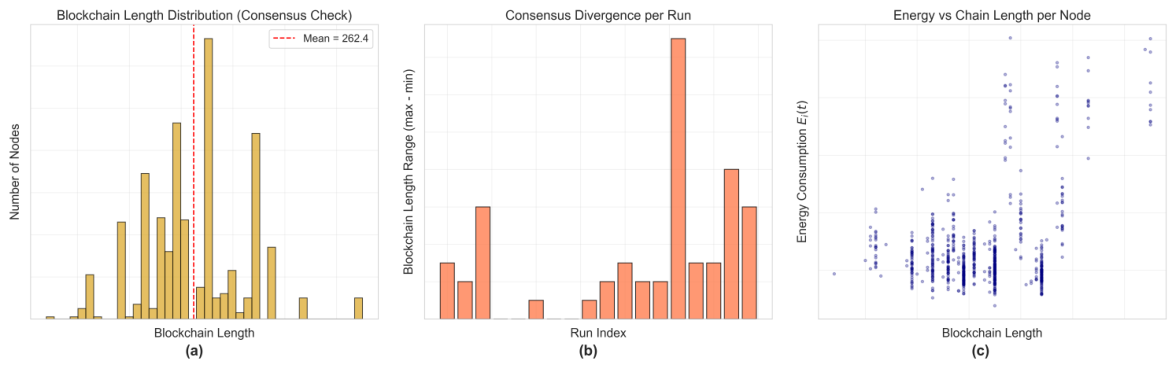
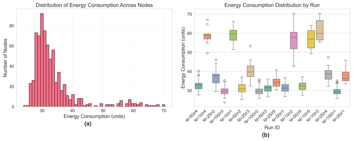
Mathematics 14 02282 g002
Figure 3. Workload capacity dynamics. The figure tests the equilibrium prediction C i = C m a x ( δ / γ ) Q i implicit in the drift of (19). (a) Scatter with X-axis: workload Q i ( t ) [transactions] and Y-axis: computational capacity C i ( t ) [normalized [ 0 , 1 ] ]; confirmed predicted inverse relation with Pearson correlation r = 0.620 . (b) Histogram X-axis: capacity C i ( t ) [normalized [ 0 , 1 ] ] Y-axis: number of observations [count] The bimodal profile (mean = 0.212 , ∼480 obs. near 0, secondary cluster near 1) suggests that the nodes are predominantly operating in a capacity-depleted regime. (c) Box plots of. Y-axis: capacity C i ( t ) [normalized]. X-axis: run identifier (N = {10, 25, 50, 100}/rk). The dependence of dispersion across runs on N is non-monotone and run dependent. (d) Plot with X-axis: theoretical equilibrium C i = C m a x ( δ / γ ) Q i [normalized]; Y-axis: measured capacity C i ( t ) [normalized]. The RMSE = 0.1147 around the identity line quantifies the agreement between the data and the equilibrium prediction.
Mathematics 14 02282 g003
Figure 4. Baseline statistical analysis of PoW energy consumption under ceteris paribus conditions (VIBES simulation, all configurations and runs). (a) Empirical density of the round energy E r with fitted Gamma distribution. (b) Average E ¯ r with 95% confidence intervals and power-law fit E ^ r n 0.350 ( R 2 = 0.997 ) (c) Q-Q plot of E r with the fitted Gamma distribution ( n = 10 , run 1). (d) Workload-capacity OLS regression Q i λ ^ κ ^ C i across all configurations. (e) Coefficient of variation and skewness of E r by configuration. (f) Notched boxplots of E r across all runs.
Mathematics 14 02282 g004
Figure 5. Consensus convergence analysis. The figure tests the ability of the gossip-based protocol to synchronize the nodes on a single chain, and if longer chains accumulate proportionally more energy. (a) Histogram with X-axis: blockchain length [blocks] and Y-axis: nodes number [count]. The peak at the mean (= 262.4 blocks) indicates that most of the nodes converge to the same tip. (b) Bar plot with X-axis: run index [dimensionless], Y-axis: chain-length range max min [blocks], near-zero values mean consensus over nodes. (c) Scatter plot with X-axis: blockchain length [blocks] and Y-axis: per-node energy consumption E i ( t ) [energy units]. The positive trend confirms the theoretical relation between cumulative mining effort and individual energy consumption.
Mathematics 14 02282 g005
Figure 6. Distribution of energy consumption. This figure tests whether homogeneous hardware/software yields homogeneous per-node energy and how this distribution varies with network size. (a) Histogram. X-axis: per-node energy consumption [energy units], Y-axis: number of nodes [count], the concentration around 28–35 units validates the homogeneity assumption (coefficient of variation = 0.31 ). (b) Box plots, X-axis: run identifier (N = {10, 25, 50, 100}/rk), Y-axis: per-node energy consumption [energy units], lower medians at larger N confirm the per-node efficiency gain reported in Table 11.
Mathematics 14 02282 g006
Figure 7. Energy decomposition analysis. The figure confirms the closed-form prediction (61) that the mining-related energy is the dominant part of the total consumption, and measures its agreement with simulation. (a) Stacked bar with X-axis: aggregate category (single bar “Average”) and Y-axis: estimated energy [energy units], decomposed into E mining = n blocks E b l o c k N (∼88%) and E val = n tx E t x N (∼12%). The dominance of the mining term shows that block-event energy dominates the budget. (b) Scatter plot with X-axis: predicted total energy from the model ( n b e 0 + n t x e t x ) · N [energy units] and Y-axis: simulated total energy E T o t [energy units]. The systematic offset below the perfect-match diagonal reveals that the analytical bound is an upper estimator.
Mathematics 14 02282 g007
Figure 8. Energy analysis: The winners and the losers The figure shows the empirical decomposition E tot = E win + E lose from (15) and the distribution of productive and wasted work over the population. (a) Bar chart with X-axis: outcome class ({Winners, Losers}) and Y-axis: aggregate energy [energy units]. The gap (23,801 vs. 624) proves that mined-chain work dominates wasted work in absolute terms. (b) Bar chart. X-axis: outcome class. Y-axis: average per-node energy [energy units]. The 25% premium (33.90 vs. 27.11) demonstrates the per-node cost asymmetry. (c) Bar chart of outcome class on the X-axis and node count [count] on the Y-axis (702 vs. 23), indicating imbalance of population. (d) Overlaid histograms X-axis: per-node energy consumption [energy units] Y-axis: number of nodes [count] Evidences cumulative-work differences between right-skewed winner distribution and lower-tail loser distribution. (e) Histogram X-axis: blocks mined per winner node [blocks] Y-axis: number of winner nodes [count] Mean = 6.80 blocks Moderate concentration of mining success. (f) Histogram, X-axis: mining efficiency [energy units/block], Y-axis: number of winner nodes [count]. Mean = 9.07 units/block. Characterizes energetic cost per successful block.
Mathematics 14 02282 g008
Figure 9. PoW Level Analysis. This figure tests the uniform participation hypothesis and the stochastic race prediction of moderate concentration of mining success. (a) Histogram of X-axis: participants per round [nodes] and Y-axis: number of rounds [count]. The discrete spikes at N { 10 , 25 , 50 , 100 } indicate complete participation in each configuration. (b) Histogram. X-axis: total energy per round [energy units]; Y-axis: number of rounds [count]. The multi-modal profile (dominant clusters near 2–3 and 6 units) reflects the four network sizes, and confirms that the round-level expenditure scales with N. (c) Bar chart with X-axis for winner node identifier (top-15) and Y-axis for rounds won [rounds]. The moderate skewness of the success distribution predicted by the stochastic race model is evidenced by the gradual decline from ∼40 to ∼30 wins.
Mathematics 14 02282 g009
Figure 10. Total wins and energy per node. This figure tests the prediction that larger hash-rate shares lead to more wins and larger cumulative energy in proportion. (a) Histogram of total PoW wins per node [wins] versus number of nodes [count]. The right-skewed profile (mode < 10 wins) is consistent with the geometric inter-arrival structure of the stochastic race. (b) Scatter with X-axis: total wins per node [wins]; Y-axis: per-node energy consumption E i ( t ) [energy units]; the strong positive linear trend proves the wins–energy proportionality. (c) Mean-with-error plot, X-axis: total wins [wins], Y-axis: average energy consumption [energy units] (error bars = standard deviation); monotone increase confirms that the relationship is robust over the observed range.
Mathematics 14 02282 g010
Figure 11. Winner vs. loser energy breakdown for the 3 highest energy rounds of the 50-node run. The figure tests whether the per-round energy burden is systemic (spread across the loser pool) or concentrated in a few nodes. Left column (a,c,e): pie charts with sectors labeled “Winner” and “Losers” and segment values reported as a percentage [%] of the total round energy (6.17 energy units per round); the near-constant 2.0–2.1% winner share vs. 97.9–98.0% loser share proves that the round burden falls overwhelmingly on losing nodes. Right column (b,d,f): pie charts decomposing the loser share, with sectors labeled by individual loser node identifier, plus a “Others” aggregate, and segment values reported as percentage [%] of loser energy; the ∼90.4% “Others” slice across all rounds proves that wasted energy is a population-wide, structural cost of PoW rather than the result of outlier nodes.
Mathematics 14 02282 g011
Figure 12. Workload division analysis. The figure describes the queue state Q i ( t ) used by the SDE (18) and verifies whether energy reacts to workload. (a) Histogram with X-axis: transaction pool size Q i ( t ) [transactions in queue] and Y-axis: number of nodes [count]; the bimodal profile (mean = 11.9 tx; spikes near 0 and 11–12) shows that nodes alternate between idle and steady state queue depths. (b) Box plots: X-axis: run identifier (N = {10, 25, 50, 100}/rk); Y-axis: transaction pool size Q i ( t ) [transactions]. Medians and dispersion show high variability between runs even for the same network size. (c) Scatter with X-axis: workload Q i ( t ) [transactions], Y-axis: per-node energy consumption E i ( t ) [energy units]. The weak positive cloud confirms the predicted but currently mild Q E coupling in case of homogeneous E t x .
Mathematics 14 02282 g012
Figure 13. Analysis of capacity change rate. The figure tests the two drift terms of the capacity SDE (19), i.e., the degradation δ i Q i and the recovery γ i ( C m a x C i ) . (a) Histogram with X-axis: rate of change of capacity d C i / d t [normalized capacity · s−1] and Y-axis: number of nodes [count]. The negative mean ( 0.004017 ) indicates that there is a net degradation under load. (b) Scatter with X-axis: workload Q i ( t ) [transactions] and Y-axis: d C i / d t [normalized capacity · s−1]; negative slope ( δ i = 0.000729 ) confirms the degradation term. (c) Scatter plot X-axis: capacity deficit ( C m a x C i ) [normalized, in [ 0 , 1 ] ] and Y-axis: d C i / d t [normalized capacity · s−1]; the fitted slope ( γ i = 0.004190 ) is non-positive, showing that under the current parameters recovery does not prevail. (d) Phase-space scatter with X-axis: workload Q i ( t ) [transactions], Y-axis: computational capacity C i ( t ) [normalized [ 0 , 1 ] ] and color: d C i / d t [normalized capacity · s−1]. The concentration at C i 0 under moderate-high Q i is persistent saturation.
Mathematics 14 02282 g013
Figure 14. Empirical Jacobian and workload–capacity linear fit ( N = 20 nodes, 26 , 945 samples, run scalability_numberOfNodes=100_run001). The figure gives an empirical calibration of the workload drift λ i κ i C i of the SDE, and tests the cross-node coupling structure of its Jacobian. (a) Scatter with X-axis: computational capacity C i [normalized [ 0 , 1 ] ] and Y-axis: workload Q i [transactions], superimposed with the linear fit Q i λ ^ κ ^ C i with λ ^ = 14.9045  tx, κ ^ = 14.1903  tx (slope 14.1903  tx per unit of normalized capacity); this gives a direct empirical value for κ i . (b) Heatmap with X-axis: capacity index j [node id 0–19], Y-axis: workload-equation index i [node id 0–19] and color: 𝜕 Q i / 𝜕 C j [tx per unit of normalized capacity, symmetric log scale]; diagonal mean = 12.0900 proves strong self-suppression, while off-diagonal mean = 0.2480 ± 0.5156 proves weak positive inter-node coupling consistent with the graph-Laplacian term of the model.
Mathematics 14 02282 g014
Figure 15. Energy vs. capacity relationship. This figure tests whether the per-node energy expenditure depends on the instantaneous capacity state–a prerequisite for the SDE’s C E coupling. (a) Scatter plot with X-axis: capacity C i ( t ) [normalized [ 0 , 1 ] ] and Y-axis: per-node energy E i ( t ) [energy units]; the very weak correlation ( r = 0.035 ) shows that under the homogeneous E b l o c k / E t x model, energy is essentially independent of capacity. (b) Bar plot with X-axis: capacity category (Very Low, Low, Medium, High, Very High) and Y-axis: average energy consumption [energy units] with std error bars. The flat ∼32–40 unit range across categories confirms the decoupling. (c) Phase-space scatter. X-axis: workload Q i ( t ) [transactions], Y-axis: capacity C i ( t ) [normalized] and color: energy E i [energy units]. The absence of a systematic gradient indicates energy is widely distributed over the state space. (d) Box plot with X-axis: capacity group ({High C i 0 , n = 725 ; Low C i < 0 , n = 0 } ) and Y-axis: per-node energy E i ( t ) [energy units]. The single populated group (IQR ≈ 28–34 units) confirms that no node ever drops below zero capacity in the current implementation.
Mathematics 14 02282 g015
Figure 16. Scalability analysis. The figure tests the linear energy scaling prediction of (23), as well as the operational invariance (throughput, latency, fork rate) of the protocol with the network growth. All four plots have the same X axis: number of nodes N { 10 , 25 , 50 , 100 } [nodes]. Error bars indicate standard deviation across runs. (a) Throughput [transactions/second] on Y-axis; ≈0.017 is almost flat, indicating that the difficulty mechanism works well at scale. (b) Y-axis: Total energy of the network (energy units). The proportional increase from 584 to 2925 units confirms the linear-aggregation identity (23). (c) Y-axis: block propagation time at the 50th percentile [seconds]; the non-monotonic profile (minimum at N = 50 ) indicates a trade-off between path redundancy and routing complexity. (d) Y-axis: blocks per run [blocks]. The N dependence indicates that the propagation-induced waste grows with the size of the network.
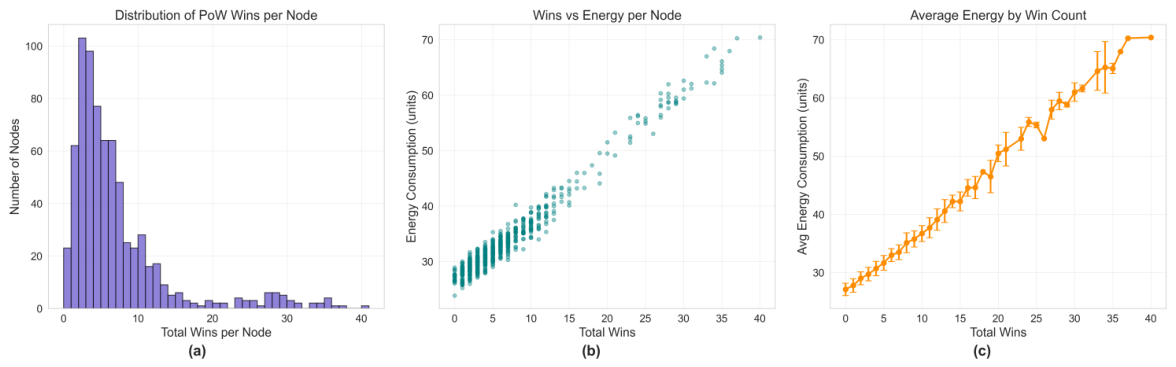
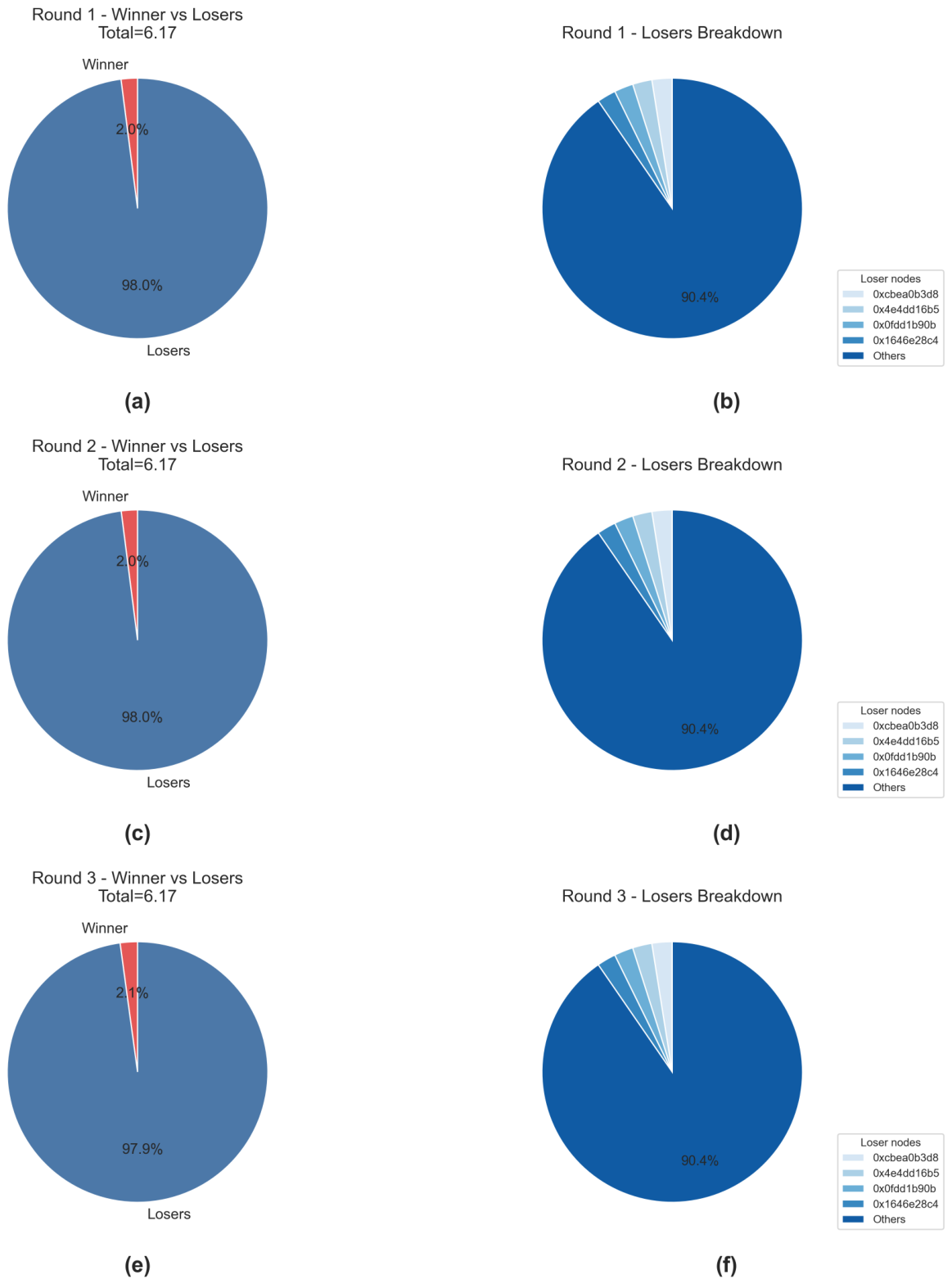
Mathematics 14 02282 g016
Figure 17. Empirical verification of the global UTXO decoupling condition (44), i.e., 𝜕 U ˙ UTXO / 𝜕 C i 0 , 𝜕 U ˙ UTXO / 𝜕 Q i 0 Each panel shows a run-level statistic ( n runs = 18 ). (a) Scatter with X-axis: mean computational capacity C i [normalized [ 0 , 1 ] ] and Y-axis: UTXO proxy U proxy [count of confirmed transactions on the longest chain]. Flat cloud ( ρ 0.059 , R 2 = 0.003 ) shows no systematic dependence. (b) Scatter plot X-axis: mean workload Q i [transactions in queue] Y-axis: U proxy [confirmed transactions, count]; the flat cloud ( ρ 0.008 , R 2 = 0.000 ) is decoupled from Q. (c) Pearson correlation matrix with X- and Y-axes: variables { C i , Q i , U proxy , N } and color: Pearson correlation [dimensionless [ 1 , 1 ] ]. The near-zero row/column for U proxy proves the decoupling jointly. The lower right inset reports raw and N-controlled partial correlations, supporting 𝜕 U ˙ UTXO / 𝜕 C i 0 and 𝜕 U ˙ UTXO / 𝜕 Q i 0 .
Mathematics 14 02282 g017aMathematics 14 02282 g017b
Table 1. Comparative summary between representative related work and the present study.
ReferenceMain Contribution in the LiteratureDifference with This Work
De Vries [3,13]Proposes macroeconomic electricity-consumption indices for Bitcoin based on profitability and hardware assumptions.We keep macro calibration as input, but model energy generation from node-level stochastic races, propagation and global state coupling.
Stoll et al. [4]Quantifies Bitcoin-related electricity demand and associated carbon emissions with regional energy-mix assumptions.We focus on the probabilistic protocol mechanisms that generate that demand, instead of only reporting aggregate annual outcomes.
Jiang et al. [5]Studies projected carbon and electricity trajectories of blockchain mining under policy and market scenarios.Our framework is process-oriented and multilevel, linking local mining behavior to semi-global competition and global energy dynamics.
Bejan et al. [6]Empirically links Bitcoin market dynamics with energy demand using data-driven modeling.We complement empirical correlation with an explicit stochastic mechanism explaining how protocol operation dissipates energy.
Sedlmeir et al. [17]Compares consensus mechanisms from an energy-efficiency perspective and discusses design trade-offs.Instead of broad consensus-family comparison, we provide a PoW-specific analytical model with local, semi-global and global layers.
Lasla et al. [20] and Yu et al. [21]Propose consensus variants aimed at reducing competitive waste and improving energy efficiency.We do not introduce a new consensus rule; we build a baseline stochastic framework to quantify where energy is spent and where waste emerges.
Decker and Wattenhofer [9]; Croman et al. [10]Characterize block propagation delays and their implications for stale blocks and scalability limits.We integrate propagation effects directly into the semi-global energy layer, connecting delay to wasted work and total expenditure.
Bowden et al. [29]; Kasahara and Kawahara [30]; Kawase and Kasahara [31]Apply stochastic and queueing models to block-arrival and confirmation-time behavior.We extend stochastic modeling toward explicit energy accounting and state-dependent power dynamics.
Eyal and Sirer [24]; Sapirshtein et al. [25]Analyze strategic mining behavior under probabilistic competition (e.g., selfish mining).We retain race-based stochastic foundations but shift the objective toward energy decomposition across operational scales.
Krause and Tolaymat [15]; CCAF [7]Provide benchmark-level estimates and datasets for blockchain electricity consumption.We use these as calibration targets while adding an endogenous stochastic structure for protocol-level energy causation.
Table 2. Typical energy sources across the three analytical scales.
LevelTypical EventsDominant VariablesMain Energetic Consequence
LocalHashing, transaction verification, relay handling, storage access h i ( r ) , Q i ( t ) , C i ( t ) Direct device-level energy expenditure by individual nodes
Semi-globalPoW races, temporary forks, block propagation, synchronization delay μ i , T , δ prop , τ Competitive overlap and stale work across interacting subsets of nodes
GlobalUTXO evolution, workload accumulation, connectivity changes, power aggregation U t , Q i ( t ) , C i ( t ) , g ( t ) , P i ( t ) System-wide energy profile and state-dependent variation in total demand
Table 3. Notation for the local and semi-global levels.
SymbolMeaning
h i ( r ) Hash rate of node i during mining round r.
pSuccess probability of one hash attempt under the current difficulty.
μ i Effective mining intensity of node i under the exponential approximation, μ i = h i ( r ) p .
T i Waiting time until node i discovers a valid block.
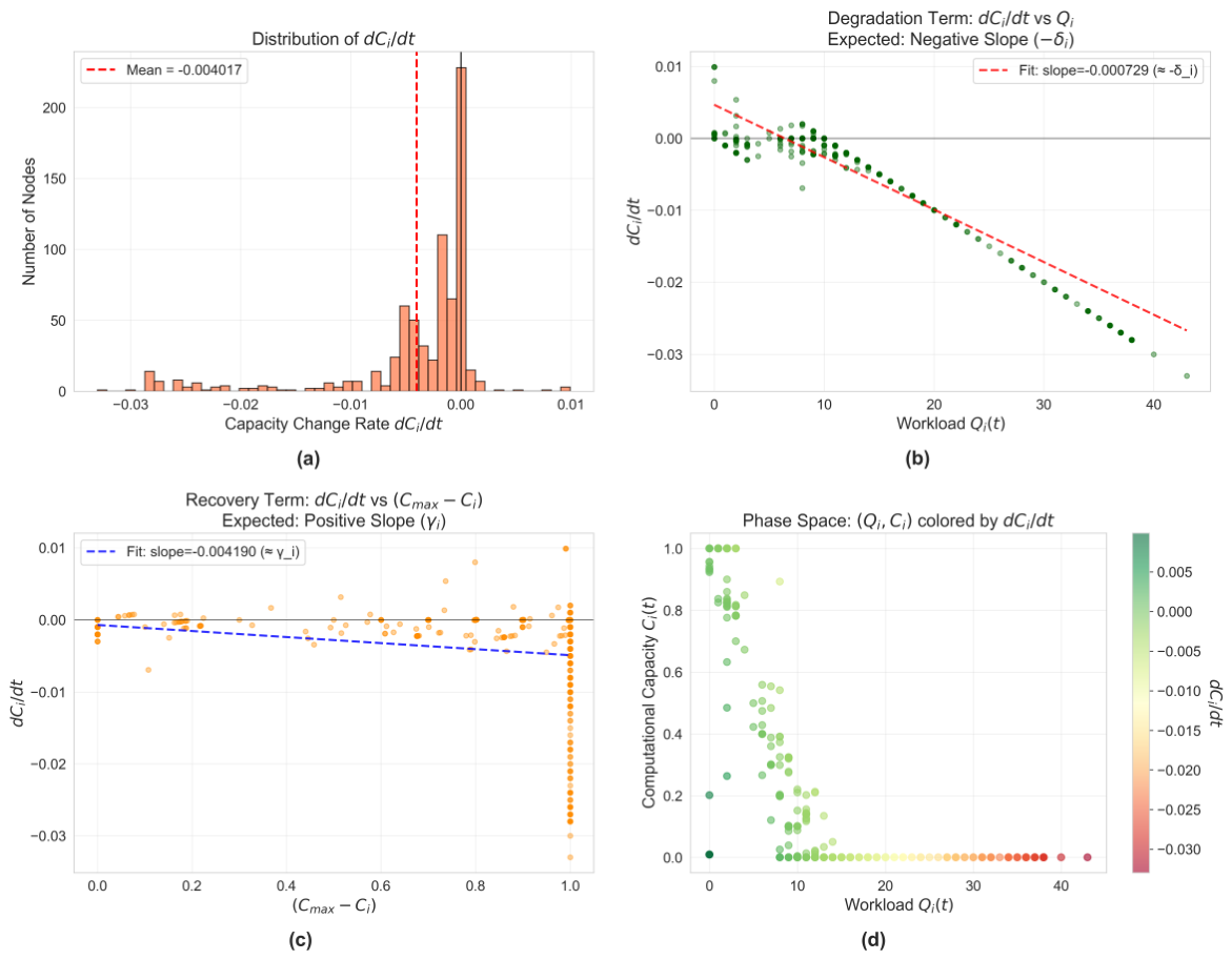
T Minimum waiting time across the active miners in one round.
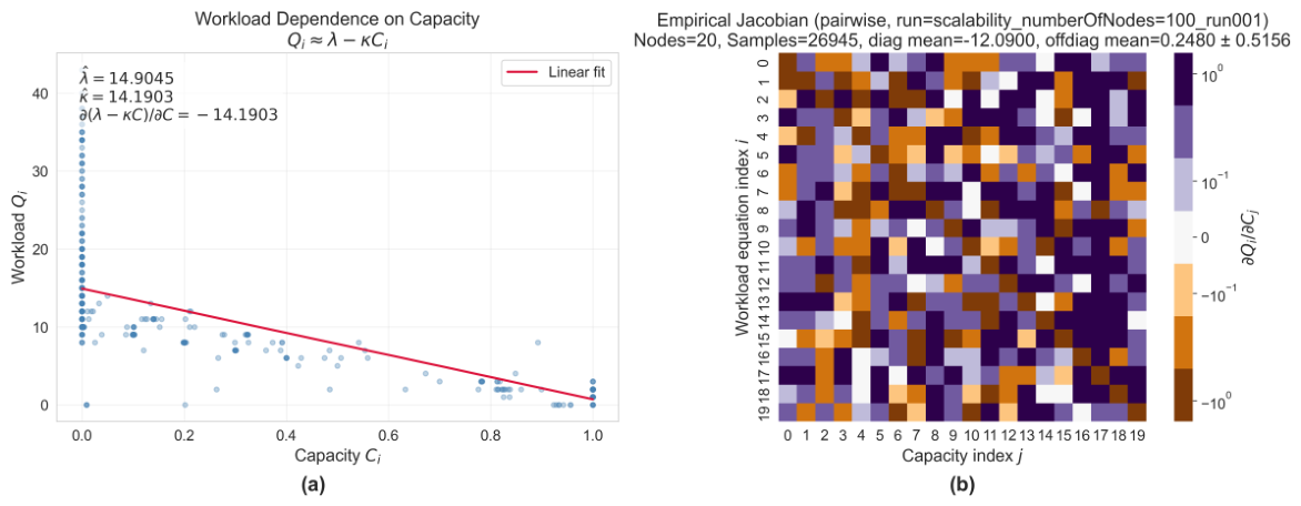
H r Set of active miners in round r.
ρ i Power consumption rate of node i while mining.
E r Total energy consumed during one mining round r.
δ prop Characteristic block propagation delay.
τ Target block interval of the protocol.
Table 4. Notation for the global stochastic layer.
SymbolMeaning
U t Size of the global UTXO population at time t.
Q i ( t ) Workload or pending-transaction state of node i in time t.
C i ( t ) Available computational capacity of node i in time t.
C max , i Maximum computational capacity of node i in time t.
g ( t ) Aggregate connectivity of the communication graph in time t.
P i ( t ) Instantaneous power consumption of node i in time t.
E Tot ( T ) Total network energy consumed over the horizon [ 0 , T ] .
λ i ( t ) Workload arrival rate at node i in time t.
𝓁 i Latent mining intensity at node i (Bayesian layer, Section 6); distinct from λ i ( t ) .
λ i , ± Jacobian eigenvalues of the workload-capacity subsystem (Section 8); distinct from λ i ( t ) .
λ Fiedler Second (Fiedler) eigenvalue of the graph Laplacian L t (Section 8.3.3); distinct from λ i ( t ) and λ i , ± .
κ i Service-rate parameter transforming capacity into workload processing.
δ i , γ i Capacity degradation and recovery coefficients.
η g , σ g Mean-reversion and volatility coefficients of aggregate connectivity.
Table 6. Illustrative action space for the node-level MDP.
ActionOperational Meaning
a mine Commit available capacity to full-intensity mining on the current candidate block.
a throttle Continue mining at reduced intensity to limit expected energy expenditure.
a validate Prioritize transaction or block verification over aggressive mining.
a relay Prioritize propagation of newly received valid data to neighbors.
a idle Remain online but temporarily abstain from energy-intensive participation.
Table 7. Interpretation of key parameter groups.
Parameter GroupInterpretationEmpirical Source
p, h i ( r ) , μ i Difficulty-governed local mining success and hash capabilityHash-rate records, difficulty data, hardware benchmarks
δ prop , τ , g ( t ) Communication quality, synchronization speed, and stale-work exposurePropagation measurements, topology studies, peer-to-peer traces
λ i , κ i , δ i , γ i Workload service, degradation, and recovery at the node levelNode logs, simulator traces, controlled performance experiments
P base , i , α comp , i , α comm , i Power baseline and sensitivity to computation and communicationHardware power profiles, facility measurements, laboratory calibration
Table 8. OLS regression Q i λ ^ κ ^ C i per network configuration. RESET: Ramsey RESET p-value for second-order non-linearity.
nN λ ^ κ ^ R 2 p ( F ) RESET p
1072913.19612.1690.482<0.0010.002
2521913.56412.5360.510<0.0010.006
5075913.62013.1530.445<0.0010.001
10067113.90613.3980.491<0.0010.005
Table 9. One-sample t-test of H 0 : E [ E r ] = e 0 / p for each network configuration. E ¯ r : observed mean round energy; μ 0 = e 0 / p : theoretical prediction under Proposition 1 with e 0 = 1 and p = 1 / n (homogeneous hash rate); α ^ : Gamma shape parameter fitted to the round-energy series.
nN E ¯ r μ 0 = e 0 / p tp-Value
107290.214410−13 113< 0.001
252190.145025−33 588< 0.001
507590.128350−142 160< 0.001
1006710.1153100−258 947< 0.001
Table 10. Overall simulation statistics (N = 18 runs).
MetricMeanStdMinMax
Number of Nodes40.2831.5510100
Actual TPS0.0170.0010.0150.018
Avg Block Time (s)650.1131.20582710
Total Energy (units)1347.22823.19558.382976.63
Avg Energy/Node40.2412.0428.9461.38
Propagation Time 50p (s)11.5610.172.041.0
Stale Blocks27.225.702041
Table 11. Scalability analysis by network size.
NodesTPSTotalEnergy/Prop.
EnergyNodeTime (s)
100.017 ± 0.001583.56 ± 22.3558.36 ± 2.2422.4 ± 12.54
250.016 ± 0.001936.07 ± 52.5937.44 ± 2.107.2 ± 4.82
500.016 ± 0.0011575.09 ± 48.8631.50 ± 0.986.4 ± 5.98
1000.017 ± 0.0002925.47 ± 44.7329.26 ± 0.459.3 ± 5.51
Disclaimer/Publisher’s Note: The statements, opinions and data contained in all publications are solely those of the individual author(s) and contributor(s) and not of MDPI and/or the editor(s). MDPI and/or the editor(s) disclaim responsibility for any injury to people or property resulting from any ideas, methods, instructions or products referred to in the content.