A Nonlinear Cross-Diffusion Model for Disease Spread: Turing Instability and Pattern Formation

Abstract

In this article, we propose a novel nonlinear cross-diffusion framework to model the distribution of susceptible and infected individuals within their habitat using a reduced SIR model that incorporates saturated incidence and treatment rates. The study investigates solution boundedness through the theory of parabolic partial differential equations, thereby validating the proposed spatio-temporal model. Through the implementation of the suggested cross-diffusion mechanism, the model reveals at least one non-constant positive equilibrium state within the susceptible–infected (SI) system. This work demonstrates the potential coexistence of susceptible and infected populations through cross-diffusion and unveils Turing instability within the system. By analyzing codimension-2 Turing–Hopf bifurcation, the study identifies the Turing space within the spatial context. In addition, we explore the results for Turing–Bogdanov–Takens bifurcation. To account for seasonal disease variations, novel perturbations are introduced. Comprehensive numerical simulations illustrate diverse emerging patterns in the Turing space, including holes, strips, and their mixtures. Additionally, the study identifies non-Turing and Turing–Bogdanov–Takens patterns for specific parameter selections. Spatial series and surfaces are graphed to enhance the clarity of the pattern results. This research provides theoretical insights into the implications of cross-diffusion in epidemic modeling, particularly in contexts characterized by localized mobility, clinically evident infections, and community-driven isolation behaviors.

1. Introduction

The theory of competing risks, which analyzes causes of death, was initially explored by Graunt in 1662. This theory has since gained firm footing among contemporary epidemiologists [1]. In 1760, Daniel Bernoulli examined the propagation of smallpox within a community using a mathematical model. In the early 20th century, William Hamer [2] and Ronald Ross [3] applied the law of mass action to elucidate the dissemination of epidemics among individuals. However, a groundbreaking advancement in the understanding of disease transmission emerged shortly after the introduction of the epidemic model proposed by Kermack and McKendrick in 1927 [4]. This model delineates the correlation between susceptible and infected individuals within a population.

The majority of researchers all around the world focus on the temporal development of epidemics with bilinear incidence rates, saturated types of incidence, and many other disease-generated interactions [5,6,7]. Additionally, researchers explore some control techniques, such as treatment and vaccines [8,9,10]. The model we consider is a SIR-type model in which the population is divided into three compartments: S (susceptible), individuals who can contract the disease; I (infected), individuals who have contracted the disease and can transmit it; and R (recovered/removed), individuals who have either recovered with immunity or died and hence do not participate in further disease transmission. Recently, Zhang et al. [7] performed a temporal analysis, including several bifurcations (backward and forward), of an SIR epidemic model, which is further explored by Gupta and Kumar [8] under the following three assumptions: (i) The susceptible and infected populations are homogeneously distributed in space; that is, these individuals are only time-dependent. (ii) The total recruitment in S-compartment is taken as constant and denoted as $\Lambda$, and (iii) both the incidence and the treatment rates are of saturated types. A flow chart for an SIR model with saturated treatment is given as follows Figure 1.

Thus, the proposed SIR model is given as follows:

$$\begin{array}{c}\hfill \left\{\begin{array}{c}{\displaystyle \frac{dS\left(t\right)}{dt}}=\Lambda -{\displaystyle \frac{\beta S\left(t\right)I\left(t\right)}{1+\mu I\left(t\right)}}-\delta S\left(t\right),\hfill \\ {\displaystyle \frac{dI\left(t\right)}{dt}}={\displaystyle \frac{\beta S\left(t\right)I\left(t\right)}{1+\mu I\left(t\right)}}-(\delta +\gamma +\sigma )I\left(t\right)-{\displaystyle \frac{\alpha I\left(t\right)}{1+\nu I\left(t\right)}},\hfill \\ {\displaystyle \frac{dR\left(t\right)}{dt}}=\gamma I\left(t\right)-\delta R\left(t\right)+{\displaystyle \frac{\alpha I\left(t\right)}{1+\nu I\left(t\right)}}\hfill \end{array}\right.\end{array}$$

(1)

with the initial condition $S\left(0\right)=S_0>0,I\left(0\right)=I_0\ge 0,R\left(0\right)=R_0>0.$ The epidemiologically meaning of the parameters used in the system (1) are given in the

Table 1. The parameters and their biological meaning.

Parameters	Biological Meaning
$\beta$	transmission rate
$\mu$	inhibitory factor
$\delta$	natural mortality rate
$\gamma$	natural recovery rate of an infected population
$\sigma$	disease-induced death rate
$\alpha$	medication rate
$\nu$	saturation factor

.

The saturated treatment rate comes into account due to the limitations of medical resources or the availability of the treatment for a particular disease. Here, it is notable that the parameter $\nu$ is the saturation factor, which quantifies the infected individual being delayed for treatment. When the number of infected individuals is low, i.e., $I\to 0$, the term approximates linear treatment, ${\displaystyle \frac{\alpha I}{1+\nu I}}\approx \alpha I$, and the healthcare system operates effectively. As the number of infectives increases, the denominator $1+\nu I$ grows, reducing the effective treatment rate per infected individual, which realistically reflects the situation when medical resources become inadequate or overloaded. The parameter $\nu$ thus regulates the decline in per-capita treatment efficacy as infection levels rise. A higher value of $\nu$ means faster saturation, indicating that even a moderate number of infections can overwhelm treatment capacity. This term is especially important when studying outbreaks in regions with limited healthcare infrastructure.

Due to biological constraints, all of these parameters are assumed to be non-negative. Gupta and Kumar [8] reduced the proposed system (1) by assuming that the third variable, R, is not present in the first two equations. They also introduced a new parameter, $ϵ=\delta +\gamma +\sigma$, that measures the disease-induced death rate after the recovery, which remains non-negative. Thus, the reduced model is given as follows:

$$\left\{\begin{array}{c}{\displaystyle \frac{dS\left(t\right)}{dt}}=\Lambda -{\displaystyle \frac{\beta S\left(t\right)I\left(t\right)}{1+\mu I\left(t\right)}}-\delta S\left(t\right),\hfill \\ {\displaystyle \frac{dI\left(t\right)}{dt}}={\displaystyle \frac{\beta S\left(t\right)I\left(t\right)}{1+\mu I\left(t\right)}}-ϵI\left(t\right)-{\displaystyle \frac{\alpha I\left(t\right)}{1+\nu I\left(t\right)}},\hfill \\ S\left(0\right)=S_0>0,I\left(0\right)=I_0\ge 0.\hfill \end{array}\right.$$

(2)

In the context of epidemiological modeling, spatial heterogeneity can play a significant role in understanding the dynamics of virus outbreaks. Spatial heterogeneity refers to variations in disease spread, population density, and other factors across different geographic regions [11,12]. If virus outbreaks were always spatially homogeneous, it would mean that the disease spreads uniformly and identically everywhere, which is rarely the case. A deterministic epidemic model in a constrained one-dimensional context, with self-diffusive spatial motion, was proposed by Webb in 1981 [13]. The author’s analysis revealed that, if the initial facts are positive, the solutions will always be well posed and positive. In order to forecast the spread of an infectious disease, the spatio-temporal dynamics of an epidemic model may be taken into account. As a result, time- and space-based mathematical models are useful to understand the spread of epidemics [12,14,15,16,17]. Thus, a reaction–diffusion process in disease dynamics deals with a disease spreading over space and time through the movement of individuals.

In particular, diffusion is known to seek an equilibrium solution in which populations are evenly dispersed [10,17,18,19]. The reaction–diffusion equations, on the other hand, may cause Turing instability and the Turing pattern [20], which is a non-equilibrium phenomenon. The authors of the articles [15,16,17,21] used epidemic models with saturated types of incidence rates and constant removal rates to study the cumulative behavior of the spatial distribution across space and time with self-diffusion. In particular, Sun et al. [15] explored an SI model with a nonlinear incidence rate and performed a Turing analysis to ensure the appearance of strip- and spot-type patterns via self-diffusion. Liu et al. [17] examined the dynamics of an epidemic model with a constant removal rate and studied how diffusion affects the emergence of spatial patterns. Further, Wang et al. [16] studied the SI model with logistic growth in susceptible individuals, using a bilinear incidence rate and diffusion to observe various types of patterns.

On the one hand, the susceptible populations always have a propensity to avoid the infected individuals in a natural setting, provided that they can recognize the infected ones due to symptoms. On the other hand, the gradient in population density of the infected compartment may cause a flux that affects the diffusion of a susceptible population. This indicates that the diffusion in one compartment affects the diffusion of the other. Cross-diffusion in mathematical models describes the effect on the motility of one species due to the presence of the other. Sun et al. [22] studied the influence of cross-diffusion on the spread of an epidemic with the help of a spatio-temporal model. According to Wang et al. [23], no Turing pattern emerges with self-diffusion for an epidemic SI model, whereas cross-diffusion develops such patterns. Even with the nonlinearity taken into account in cross-diffusive terms, its impact on various populations is still similar. In order to replicate this scenario in our study, we have created novel, nonlinear, complex cross-diffusion with both quadratic and rational factors for both the susceptible and infected classes.

In general, a vulnerable individual takes precautions to avoid getting into contact with a person infected with a communicable disease like COVID-19, AIDS, etc. Additionally, the mobility of people is impacted by media coverage and health ministry awareness, which cannot be captured through simple cross-diffusion. These elements cannot be disregarded if one wants to learn more about disease transmission. Though many researchers consider nonlinear cross-diffusion using the standard heat equation, very few researchers focus on disease dissemination in an environment with nonlinear cross-diffusion. Fortunately, some research studies have been suggested that have examined nonlinear cross-diffusion for a set of reaction–diffusion equations for various interacting population models [24,25,26,27,28,29]. In particular, cross-diffusion and self-diffusion models were originally proposed by Shigesada et al. [27] to model the spatial segregation of two competing species. The key characteristic of this model was to demonstrate that, if random diffusion alone is unable to result in the spatial segregation of two competing species, then perhaps a nonlinear dispersal approach can. Further, Ni et al. [30] proposed a non-linear cross-diffusion and analyzed the spike-layer equilibrium state. In the article [26], the authors also studied the effect of cross-diffusion in a second species and showed that the flux of the second species is directed towards the decreasing population density of the first species. Recently, Zhou et al. [29] analyzed a cooperative two-species Lotka–Volterra model to demonstrate that, if birth rates are high and cross-diffusions are suitably weak, the model has at least one coexisting state. This literature suggests that the proposed nonlinear cross-diffusion terms may be constituents that are quadratic [31], rational [24], or a combination of both [29].

A variety of diffusion rates across many decades of mathematical modeling have been utilized. Motivated by the above-cited works, we have proposed nonlinear cross-diffusion, on the basis of which the dissemination of susceptible and infected populations depends on the movement of each class, as follows:

$$F_1(S,I)=\left({\delta }_{11}+{\delta }_{12}S+{\displaystyle \frac{{\beta }_{11}I}{1+{\mu }_{11}I}}\right)S,F_2(S,I)=\left({\delta }_{21}+{\delta }_{22}I+{\displaystyle \frac{{\beta }_{22}S}{1+{\mu }_{22}S}}+{\displaystyle \frac{{\alpha }_{21}}{1+{\alpha }_{22}I}}\right)I.$$

Here, ${\delta }_{ij}$ (for $i,j=1,2$), ${\beta }_{11}$, ${\beta }_{22}$, ${\mu }_{11}$, ${\mu }_{22}$, ${\alpha }_{21}$, and ${\alpha }_{22}$ are the positive diffusive constants; due to these parameters, the influences on self- and cross-diffusion is affected. Also, we notice the following:

• For ${\alpha }_{21}={\delta }_{12}=0={\mu }_{11}={\mu }_{22}={\delta }_{22}$, cross-diffusion is similar to that described in the article [25];
• For ${\mu }_{11}=0={\alpha }_{21}={\mu }_{22}$, the diffusion is the same as in the article [31];
• For ${\delta }_{12}={\beta }_{11}=0={\delta }_{22}={\beta }_{22}={\alpha }_{21}$, the diffusion is of the self-type. Many researchers [15,16,17] studied the effect of self-diffusion in the distribution of various species in many branches of mathematical modeling. Here, it is notable that the roles of S and I will be changed according to the species of these models.

In the diffusion term $\Delta F_1(S,I)=\nabla ·\left\{\left({\delta }_{11}+2{\delta }_{12}S+{\displaystyle \frac{{\beta }_{11}I}{1+{\mu }_{11}I}}\right)\nabla S+{\displaystyle \frac{{\beta }_{11}S}{{(1+{\mu }_{11}I)}^2}}\nabla I\right\},$ the first term $\left({\delta }_{11}+2{\delta }_{12}S+{\displaystyle \frac{{\beta }_{11}I}{1+{\mu }_{11}I}}\right)$ represents self-diffusion, as it influences the term $\nabla S$ of the gradient. In an interacting environment, the self-diffusion for the movement of a susceptible population depends on the density of infected individuals and vice versa. The cross-diffusion term ${\displaystyle \frac{{\beta }_{11}S}{{(1+{\mu }_{11}I)}^2}}$ influences the interaction between susceptible and infected populations. Crowding’s hindrance of movement can be incorporated by introducing the current population density of infected individuals in the denominator of the fractional part of the cross-diffusion term [32]. Also, if the population density of either S or I increases, it will make movement difficult. The flux of $F_2(S,I)$ is $\Delta F_2(S,I)=\nabla ·\left\{{\displaystyle \frac{{\beta }_{22}I}{{(1+{\mu }_{22}S)}^2}}\nabla S+\left({\delta }_{21}+2{\delta }_{22}I+{\displaystyle \frac{{\beta }_{22}S}{1+{\mu }_{22}S}}+{\displaystyle \frac{{\alpha }_{21}}{{(1+{\alpha }_{22}I)}^2}}\right)\nabla I\right\}$, which is replicated the same as in the earlier case.

Quadratic terms ($2{\delta }_{12}S$, $2{\delta }_{22}I$): These account for density-dependent movement pressure. For example, the term $2{\delta }_{12}S\nabla S$ in the first equation suggests that the movement of susceptible individuals increases nonlinearly with their own density, possibly due to crowding, competition for resources, or social interaction.

Saturated terms (e.g., ${\displaystyle \frac{{\beta }_{11}I}{1+{\mu }_{11}I}}$, ${\displaystyle \frac{{\beta }_{22}S}{1+{\mu }_{22}S}}$, ${\displaystyle \frac{{\alpha }_{21}}{{(1+{\alpha }_{22}I)}^2}}$): These describe limited or saturating behavioral responses. For instance, the rate at which susceptible individuals respond to infected individuals (via the gradient of I) is modulated through ${\displaystyle \frac{{\beta }_{11}I}{1+{\mu }_{11}I}}$, implying that their reaction saturates as the infected population grows. This reflects realistic constraints such as a limited avoidance ability, immune fatigue, or bounded information processing.

Mixed-gradient terms (e.g., $\nabla I$ in $\Delta F_1$ and $\nabla S$ in $\Delta F_2$): These terms indicate the behavioral responses of one class to the spatial gradient of the other—for example, susceptible individuals moving in response to spatial variation in infected density. The saturated structure again ensures realistic movement bounds.

We have demonstrated, through flux calculations, that our cross-diffusion is an indication of the propensity of the vulnerable population to avoid the infected ones. As far as our knowledge goes, this form of cross-diffusion is not available in the literature.

As a result, the system (2) with described nonlinear cross-diffusive functions over $\Omega \times T$ ($\Omega \subset {\mathbb{R}}_{+}^2$) can be written as

$$\begin{array}{c}\hfill \left\{\begin{array}{c}{\displaystyle \frac{\partial S(x,t)}{\partial t}}=\Delta F_1\left(S,I\right)+\Lambda -{\displaystyle \frac{\beta S(x,t)I(x,t)}{1+\mu I(x,t)}}-\delta S(x,t),\hfill \\ {\displaystyle \frac{\partial I(x,t)}{\partial t}}=\Delta F_2\left(S,I\right)+{\displaystyle \frac{\beta S(x,t)I(x,t)}{1+\mu I(x,t)}}-ϵI(x,t)-{\displaystyle \frac{\alpha I(x,t)}{1+\nu I(x,t)}}\hfill \end{array}\right.\end{array}$$

(3)

with the following initial and boundary conditions:

$$\begin{array}{c}\hfill \left\{\begin{array}{c}{\displaystyle \frac{\partial S(x,t)}{\partial n}}={\displaystyle \frac{\partial I(x,t)}{\partial n}}=0,x\in \partial \Omega ,t>0,t\in [0,T],\hfill \\ S(x,0)=S_0\left(x\right)\ge 0,I(x,0)=I_0\left(x\right)\ge 0,x\in \Omega .\hfill \end{array}\right.\end{array}$$

(4)

Here, the boundary condition is taken as the Neumann type. The parameter n denotes the outward normal unit vector for the domain $\Omega$. In order to explore the system (3) for the effect of cross-diffusion between susceptible and infected populations due to their movement, the remaining part of this manuscript is arranged in the following order. Next, in Section 2, we analyze the boundedness of solutions to the system (3). The existence and non-existence of non-constant equilibrium states and constant equilibrium states are determined in Section 3.1 and Section 3.2, respectively. Through the existence of codimension-2 Turing–Hopf bifurcation, followed by a spatial analysis and Turing instability, we determine the Turing space in the spatial domain in Section 4. An extensive numerical simulation is performed in Section 5 to obtain the various patterns, such as Turing, non-Turing, Turing–Hopf, and Turing–Bogdanov–Takens patterns. In the last part of the manuscript, we discuss the main results in Section 6.

2. Boundedness of Solutions

Now, we determine the boundedness of solutions for the system (3) using Lemma 2.1 from [33].

Theorem 1.

For a constant ${\Lambda }_1>0$ (depends on initial data), the solution of the system (3) satisfies ${\parallel S(·,t)\parallel }_{L^1(\Omega )}+{\parallel I(·,t)\parallel }_{L^1(\Omega )}\le {\Lambda }_1,\forall t\ge 0.$ Additionally, for a sufficiently large T, there exists a constant, ${\Lambda }_2$ (independent of initial data), such that ${\parallel S(·,t)\parallel }_{L^{\infty }(\Omega )}+{\parallel I(·,t)\parallel }_{L^{\infty }(\Omega )}\le {\Lambda }_2,\forall t\ge T.$

Proof. 

Adding both equations of the system (3), we get

$$\begin{array}{cc}\hfill {\displaystyle \frac{\partial S}{\partial t}}+{\displaystyle \frac{\partial I}{\partial t}}=& \nabla ·\left\{\left({\delta }_{11}+2{\delta }_{12}S+{\displaystyle \frac{{\beta }_{11}I}{1+{\mu }_{11}I}}\right)\nabla S+{\displaystyle \frac{{\beta }_{11}S}{{(1+{\mu }_{11}I)}^2}}\nabla I\right\}+\Lambda -ϵI-\delta S-{\displaystyle \frac{\alpha I}{1+\nu I}}\hfill \\ & +\nabla ·\left\{{\displaystyle \frac{{\beta }_{22}I}{{(1+{\mu }_{22}S)}^2}}\nabla S+\left({\delta }_{21}+2{\delta }_{22}I+{\displaystyle \frac{{\beta }_{22}S}{1+{\mu }_{22}S}}+{\displaystyle \frac{{\alpha }_{21}}{{(1+{\alpha }_{22}I)}^2}}\right)\nabla I\right\}.\hfill \end{array}$$

(5)

On integrating Equation (5) over the region $\Omega$, we obtain

$$\begin{array}{cc}\hfill {\int }_{\Omega }\left({\displaystyle \frac{\partial S}{\partial t}}+{\displaystyle \frac{\partial I}{\partial t}}\right)dx=& {\int }_{\Omega }\left[\nabla ·\left\{\left({\delta }_{11}+2{\delta }_{12}S+{\displaystyle \frac{{\beta }_{11}I}{1+{\mu }_{11}I}}\right)\nabla S+{\displaystyle \frac{{\beta }_{11}S}{{(1+{\mu }_{11}I)}^2}}\nabla I\right\}-\delta S-{\displaystyle \frac{\alpha I}{1+\nu I}}\right.\hfill \\ & \left.+\Lambda -ϵI+\nabla ·\left\{{\displaystyle \frac{{\beta }_{22}I}{{(1+{\mu }_{22}S)}^2}}\nabla S+\left({\delta }_{21}+2{\delta }_{22}I+{\displaystyle \frac{{\beta }_{22}S}{1+{\mu }_{22}S}}+{\displaystyle \frac{{\alpha }_{21}}{{(1+{\alpha }_{22}I)}^2}}\right)\nabla I\right\}\right]dx.\hfill \end{array}$$

Let

$$U\left(t\right)={\int }_{\Omega }[S(x,t)+I(x,t)]dx,\forall t\ge 0,$$

differentiate it with respect to t, we get

$${\displaystyle \frac{dU\left(t\right)}{dt}}={\int }_{\Omega }\left({\displaystyle \frac{\partial S}{\partial t}}+{\displaystyle \frac{\partial I}{\partial t}}\right)dx.$$

Using the Gauss and Green’s identity as $\Delta \left(\overrightarrow{\mathbf{X}}\right)=\nabla ·(\nabla \overrightarrow{\mathbf{X}})$ and ${\int }_{\Omega }\nabla ·(\nabla \overrightarrow{\mathbf{X}})={\int }_{\partial \Omega }(\nabla \overrightarrow{\mathbf{X}})·\widehat{n}$, we conclude

$$\begin{array}{cc}\hfill {\displaystyle \frac{dU\left(t\right)}{dt}}=& {\int }_{\Omega }\left[\Lambda -ϵI-\delta S-{\displaystyle \frac{\alpha I}{1+\nu I}}\right]dx\hfill \\ & +{\int }_{\partial \Omega }\left[\left({\displaystyle \frac{{\beta }_{11}S}{{(1+{\mu }_{11}I)}^2}}+{\delta }_{21}+2{\delta }_{22}I+{\displaystyle \frac{{\beta }_{22}S}{1+{\mu }_{22}S}}+{\displaystyle \frac{{\alpha }_{21}}{{(1+{\alpha }_{22}I)}^2}}\right)\widehat{n}·(\nabla I)\right.\hfill \\ & \left.+\left({\displaystyle \frac{{\beta }_{11}I}{1+{\mu }_{11}I}}+{\delta }_{11}+2{\delta }_{12}S+{\displaystyle \frac{{\beta }_{22}I}{{(1+{\mu }_{22}S)}^2}}\right)\widehat{n}·(\nabla S)\right].\hfill \end{array}$$

(6)

Under the Neumann boundary condition (4), we have $\widehat{n}·(\nabla S)=0=\widehat{n}·(\nabla I)$. Set $\Psi =min(\delta ,ϵ)$, so that the above Equation (6) reduces to

$${\displaystyle \frac{dU\left(t\right)}{dt}}\le -\Psi U\left(t\right)+{\int }_{\Omega }\Lambda dx,\forall t\ge 0.$$

This is equivalent to

$$U\left(t\right)\le U\left(0\right)e^{-\Psi t}+{\displaystyle \frac{|\Omega |}{\Psi }}\Lambda (1-e^{-\Psi t}),\forall t\ge 0.$$

(7)

In the inequality (7) using Lemma 2.1 of [33] and positivity of S and I, we obtain

$${\parallel S(·,t)\parallel }_{L^1(\Omega )}+{\parallel I(·,t)\parallel }_{L^1(\Omega )}\le {\Lambda }_1,\forall t\ge 0.$$

Furthermore, from the inequality (7), we deduce that ${lim}_{\begin{array}{c}t\to \infty \end{array}}sup\left|U\left(t\right)\right|\le {\displaystyle \frac{|\Omega |}{\Psi }}\Lambda .$ Thus, we conclude that there exists a positive constant, ${\Lambda }_2$, such that ${\parallel S(·,t)\parallel }_{L^{\infty }(\Omega )}+{\parallel I(·,t)\parallel }_{L^{\infty }(\Omega )}\le {\Lambda }_2,\forall t\ge T,$ for a sufficiently large time, $T>0$. □

3. Analysis of Endemic State

In a reaction–diffusion system, two types of equilibrium states can exist: the first is a constant equilibrium state, which occurs when both the spatial and temporal derivatives vanish, and the second is a non-constant equilibrium state, which occurs when only the temporal derivative becomes zero, while spatial variations remain. In this section, we study both the constant and non-constant endemic equilibrium states for the system (3).

The system (3) transforms into a strongly coupled elliptic system when ${\displaystyle \frac{\partial S(x,t)}{\partial t}}=0={\displaystyle \frac{\partial I(x,t)}{\partial t}}$. Such equations have garnered significant attention in recent years [24,29,34,35,36]. Previous works [37,38] employed bifurcation theory to investigate the coexistence of equilibrium states in coupled elliptic systems. Notably, Ryu and Ahn [39] utilized fixed point indices to demonstrate the existence of positive solutions in a two-equation system with density-dependent diffusions. Pao [40] demonstrated that solutions to a broad class of coupled elliptic equations can be obtained through the method of upper and lower solutions and associated monotone iterations. Building upon this foundation, our research is motivated by the question of the existence of a solution for the coupled elliptic system. A comprehensive discussion is presented in Section 3.1.

3.1. Existence and Non-Existence of Non-Constant Endemic State

The coexistence of solutions in the elliptic differential system (3) signifies the persistent presence of both populations within a specific environmental habitat. The emergence of patterns relies on population coexistence. “In practice, boundary conditions simplify the mathematical representation of interactions. Dirichlet boundary conditions prescribe variable values at the domain boundary, useful in closed environments like nursing homes or hospitals, representing population density constraints. Neumann boundary conditions, allowing more flexibility, are suitable when specifying boundary values is impractical or irrelevant [41]. In our study, using Dirichlet’s boundary condition demonstrates the coexistence of populations, particularly relevant for closed environments.” Consequently, the coupled elliptic system corresponding to the model (3) with a Dirichlet boundary condition is given as

$$\begin{array}{c}\hfill \left\{\begin{array}{c}0=\Delta F_1\left(S,I\right)+\Lambda -{\displaystyle \frac{\beta S\left(x\right)I\left(x\right)}{1+\mu I\left(x\right)}}-\delta S\left(x\right),\hfill \\ 0=\Delta F_2\left(S,I\right)+{\displaystyle \frac{\beta S\left(x\right)I\left(x\right)}{1+\mu I\left(x\right)}}-ϵI\left(x\right)-{\displaystyle \frac{\alpha I\left(x\right)}{1+\nu I\left(x\right)}},\hfill \\ S\left(x\right)=0\mathrm{and}I\left(x\right)=0,x\in \partial \Omega .\hfill \end{array}\right.\end{array}$$

(8)

To obtain a sufficient condition for coexistence, rewrite the system (8) as follows:

$$\begin{array}{c}\hfill \left\{\begin{array}{c}-\Delta F_1\left(S,I\right)=G_1(S,I),x\in \Omega ,\hfill \\ -\Delta F_2\left(S,I\right)=G_2(S,I),x\in \Omega ,\hfill \\ S\left(x\right)=0\mathrm{and}I\left(x\right)=0,x\in \partial \Omega ,\hfill \end{array}\right.\end{array}$$

(9)

where $G_1(S,I)=\Lambda -{\displaystyle \frac{\beta S\left(x\right)I\left(x\right)}{1+\mu I\left(x\right)}}-\delta S\left(x\right)$ and $G_2(S,I)={\displaystyle \frac{\beta S\left(x\right)I\left(x\right)}{1+\mu I\left(x\right)}}-ϵI\left(x\right)-{\displaystyle \frac{\alpha I\left(x\right)}{1+\nu I\left(x\right)}}.$ Proceeding similarly to Pao [40], we investigate the existence of positive solutions for the coupled Equation (9) by defining $U=F_1\left(S,I\right)$ and $V=F_2\left(S,I\right)$. The determinant of the Jacobian of the transformations U and V is given by

$$\begin{array}{cc}\hfill \left|J\right|=& \left|{\displaystyle \frac{\partial (U,V)}{\partial (S,I)}}\right|=\left[\left({\delta }_{11}+{\displaystyle \frac{{\beta }_{11}I}{1+{\mu }_{11}I}}+2{\delta }_{12}S\right)\left(2{\delta }_{22}I+{\delta }_{21}+{\displaystyle \frac{{\alpha }_{21}}{{(1+{\alpha }_{22}I)}^2}}\right)\right.\hfill \\ & \left.+{\displaystyle \frac{{\beta }_{11}{\beta }_{22}SI({\mu }_{22}S+{\mu }_{11}I+{\mu }_{11}{\mu }_{22}SI)}{{(1+{\mu }_{22}S)}^2{(1+{\mu }_{11}I)}^2}}+{\displaystyle \frac{{\beta }_{22}S\left(2{\delta }_{22}I+{\delta }_{21}\right)}{1+{\mu }_{22}S}}\right]>0,\forall (S,I)\ge (0,0).\hfill \end{array}$$

Hence, from the inverse function theorem, there exist $S=H_1(U,V)$ and $I=H_2(U,V)$ for $(S,I)\ge (0,0)$. Thus, the system (9) can be written as

$$\begin{array}{c}\hfill \left\{\begin{array}{c}-\Delta U+K_{1}U={\tilde{G}}_1(S,I),x\in \Omega ,\hfill \\ -\Delta V+K_{2}V={\tilde{G}}_2(S,I),x\in \Omega ,\hfill \\ S=H_1(U,V)\mathrm{and}I=H_2(U,V),x\in \Omega ,\hfill \\ U\left(x\right)=0\mathrm{and}V\left(x\right)=0,x\in \partial \Omega ,\hfill \end{array}\right.\end{array}$$

where ${\tilde{G}}_i(S,I)=K_i{F}_i(S,I)+G_i(S,I)$ for $i=1,2$. We assume $K_1{\delta }_{11}-\delta >{\displaystyle \frac{\beta }{\mu }}$ and $K_2>{\displaystyle \frac{ϵ+\alpha }{{\delta }_{21}}}$ to get

$${\displaystyle \frac{\partial {\tilde{G}}_1(S,I)}{\partial S}}=K_1\left({\delta }_{11}+{\displaystyle \frac{{\beta }_{11}I}{1+{\mu }_{11}I}}+2{\delta }_{12}S\right)-{\displaystyle \frac{\beta I}{1+\mu I}}-\delta \ge 0,$$

$${\displaystyle \frac{\partial {\tilde{G}}_1(S,I)}{\partial I}}=K_1\left({\displaystyle \frac{{\beta }_{11}S}{{(1+{\mu }_{11}I)}^2}}\right)-{\displaystyle \frac{\beta S}{{(1+\mu I)}^2}},$$

$${\displaystyle \frac{\partial {\tilde{G}}_2(S,I)}{\partial S}}=K_2\left({\displaystyle \frac{{\beta }_{22}I}{{(1+{\mu }_{22}S)}^2}}\right)+{\displaystyle \frac{\beta I}{1+\mu I}}\ge 0\mathrm{and}$$

$${\displaystyle \frac{\partial {\tilde{G}}_2(S,I)}{\partial I}}=K_2\left(2{\delta }_{22}I+{\delta }_{21}+{\displaystyle \frac{{\beta }_{22}S}{1+{\mu }_{22}S}}+{\displaystyle \frac{{\alpha }_{21}}{{(1+{\alpha }_{22}I)}^2}}\right)+{\displaystyle \frac{\beta S}{{(1+\mu I)}^2}}-ϵ-{\displaystyle \frac{\alpha }{{(1+\nu I)}^2}}\ge 0.$$

It is clear that ${\tilde{G}}_1(S,I)$ is non-decreasing in S, and ${\tilde{G}}_2(S,I)$ is non-decreasing in S and I. The sign of ${\displaystyle \frac{\partial {\tilde{G}}_1(S,I)}{\partial I}}$ cannot be obtained easily. On the other hand, an elementary calculations yields

$${\displaystyle \frac{\partial S}{\partial U}}=\left(2{\delta }_{22}I+{\delta }_{21}+{\displaystyle \frac{{\beta }_{22}S}{1+{\mu }_{22}S}}+{\displaystyle \frac{{\alpha }_{21}}{{(1+{\alpha }_{22}I)}^2}}\right)/\left|J\right|,{\displaystyle \frac{\partial I}{\partial U}}=\left({\displaystyle \frac{{\beta }_{22}I}{{(1+{\mu }_{22}S)}^2}}\right)/\left|J\right|,$$

$${\displaystyle \frac{\partial S}{\partial V}}=\left({\displaystyle \frac{{\beta }_{11}S}{{(1+{\mu }_{11}I)}^2}}\right)/\left|J\right|,{\displaystyle \frac{\partial I}{\partial V}}=\left({\delta }_{11}+{\displaystyle \frac{{\beta }_{11}I}{1+{\mu }_{11}I}}+2{\delta }_{12}S\right)/\left|J\right|.$$

This shows that $H_i(U,V)$ for $i=1,2$ is non-decreasing in U and V, whenever $(U,V)>(0,0)$. We define two sets, $\overline{M}=\{P\in C^2\overline{(\Omega )}:\widehat{P}\le P\le \tilde{P}\}$ and $\underline{M}=\{Q\in C^2\overline{(\Omega )}:\widehat{Q}\le Q\le \tilde{Q}\}$, where $P=(S,I),\tilde{P}=(\tilde{S},\tilde{I}),\widehat{P}=(\widehat{S},\widehat{I})$, and $Q=(U,V),\tilde{Q}=(\tilde{U},\tilde{V}),\widehat{Q}=(\widehat{U},\widehat{V})$. For $x\in \Omega$, we call the pair $(\tilde{S},\tilde{I})$ and $(\widehat{S},\widehat{I})$ the coupled upper and lower solutions of the system (9) if they satisfy

$$\begin{array}{c}\hfill \left\{\begin{array}{c}-\Delta \left[F_1(\tilde{S},\widehat{I})\right]+K_1{F}_1(\tilde{S},\widehat{I})\ge {\tilde{G}}_1(\tilde{S},\tilde{I}),\hfill \\ -\Delta \left[F_2(\widehat{S},\tilde{I})\right]+K_2{F}_2(\widehat{S},\tilde{I})\ge {\tilde{G}}_2(\tilde{S},\tilde{I}),\hfill \\ -\Delta \left[F_1(\widehat{S},\tilde{I})\right]+K_1{F}_1(\widehat{S},\tilde{I})\le {\tilde{G}}_1(\widehat{S},\widehat{I}),\hfill \\ -\Delta \left[F_2(\tilde{S},\widehat{I})\right]+K_2{F}_2(\tilde{S},\widehat{I})\le {\tilde{G}}_2(\widehat{S},\widehat{I})\hfill \end{array}\right.\end{array}$$

(10)

with $\tilde{S}\left(x\right)\ge 0=\widehat{S}\left(x\right),\tilde{I}\left(x\right)\ge 0=\widehat{I}\left(x\right),x\in \partial \Omega$ and $(\tilde{S},\tilde{I})\ge (\widehat{S},\widehat{I})$. For a more precise definition of coupled upper and lower solutions, please see [42]. Now, we seek a pair of coupled upper solutions of (9) in the form $(\tilde{S},\tilde{I})=(M_1,M_2)$, where $M_1$ and $M_2$ are some positive constants. Further, we consider a lower solution of the system (9) as $(\widehat{S},\widehat{I})=(H_1({\theta }_1\varphi ,{\theta }_2\varphi ),H_2({\theta }_1\varphi ,{\theta }_2\varphi )),$ where ${\theta }_i$$(\mathrm{for}i=1,2)$ are sufficiently small positive constants, and $\varphi =\varphi \left(x\right)$ is the normalized positive eigenfunction corresponding to the smallest eigenvalue, ${\lambda }_0$, of the Laplacian $\Delta$ under the Dirichlet boundary condition. Indeed, $(M_1,M_2)$ and $({\theta }_1\varphi ,{\theta }_2\varphi )$ satisfy the first two conditions of system (10) if

$$\begin{array}{c}\hfill \left\{\begin{array}{c}-\Delta \left[F_1(M_1,{\theta }_2\varphi )\right]\ge G_1(M_1,M_2)+K_1\left({\displaystyle \frac{{\beta }_{11}{M}_2}{1+{\mu }_{11}{M}_2}}-{\displaystyle \frac{{\beta }_{11}{\theta }_2\varphi }{1+{\mu }_{11}{\theta }_2\varphi }}\right)M_1,\hfill \\ -\Delta \left[F_2({\theta }_1\varphi ,M_2)\right]\ge G_2(M_1,M_2)+K_2\left({\displaystyle \frac{{\beta }_{22}{M}_1}{1+{\mu }_{22}{M}_2}}-{\displaystyle \frac{{\beta }_{22}{\theta }_1\varphi }{1+{\mu }_{22}{\theta }_1\varphi }}\right)M_2.\hfill \end{array}\right.\end{array}$$

(11)

This is equivalent to

$$\begin{array}{c}\hfill \left\{\begin{array}{c}-\Delta \left[\left({\delta }_{11}+{\delta }_{12}{M}_1+{\displaystyle \frac{{\beta }_{11}{\theta }_2\varphi }{1+{\mu }_{11}{\theta }_2\varphi }}\right)M_1\right]\ge \Lambda -{\displaystyle \frac{\beta M_1{M}_2}{1+\mu M_2}}-\delta M_1+K_1\left({\displaystyle \frac{{\beta }_{11}{M}_2}{1+{\mu }_{11}{M}_2}}-{\displaystyle \frac{{\beta }_{11}}{{\mu }_{11}}}\right)M_1,\hfill \\ -\Delta \left[\left({\delta }_{21}+{\delta }_{22}{M}_2+{\displaystyle \frac{{\beta }_{22}{\theta }_1\varphi }{1+{\mu }_{22}{\theta }_1\varphi }}+{\displaystyle \frac{{\alpha }_{21}}{1+{\alpha }_{22}{M}_2}}\right)M_2\right]\ge {\displaystyle \frac{\beta M_1{M}_2}{1+\mu M_2}}-ϵM_2-{\displaystyle \frac{\alpha M_2}{1+\nu M_2}}\hfill \\ +K_2\left({\displaystyle \frac{{\beta }_{22}{M}_1}{1+{\mu }_{22}{M}_1}}-{\displaystyle \frac{{\beta }_{22}}{{\mu }_{22}}}\right)M_2.\hfill \end{array}\right.\end{array}$$

(12)

In fact, the inequalities of the system (12) hold if

$$\begin{array}{c}\hfill \left\{\begin{array}{c}0\ge \Lambda -\delta M_1-{\displaystyle \frac{\beta M_1}{\mu }}+K_1\left({\displaystyle \frac{{\beta }_{11}}{{\mu }_{11}}}-{\displaystyle \frac{{\beta }_{11}{M}_2}{1+{\mu }_{11}{M}_2}}\right)M_1,\hfill \\ 0\ge {\displaystyle \frac{\beta M_1}{1+\mu M_2}}-ϵ-{\displaystyle \frac{\alpha }{\nu }}+K_2\left({\displaystyle \frac{{\beta }_{22}}{{\mu }_{22}}}-{\displaystyle \frac{{\beta }_{22}{M}_1}{1+{\mu }_{22}{M}_1}}\right).\hfill \end{array}\right.\end{array}$$

(13)

Again, the upper and lower solutions $(M_1,M_2)$ and $({\theta }_1\varphi ,{\theta }_2\varphi )$ satisfy the last two conditions of system (10) if

$$\begin{array}{c}\hfill \left\{\begin{array}{c}-\Delta \left({\delta }_{11}+{\delta }_{12}{\theta }_1\varphi +{\displaystyle \frac{{\beta }_{11}{M}_2}{1+{\mu }_{11}{M}_2}}\right){\theta }_1\varphi \le \left[K_1{\theta }_1\varphi \left({\displaystyle \frac{{\beta }_{11}\widehat{I}}{1+{\mu }_{11}\widehat{I}}}-{\displaystyle \frac{{\beta }_{11}{M}_2}{1+{\mu }_{11}{M}_2}}\right)+\Lambda -{\displaystyle \frac{\beta {\theta }_1{\varphi }^2{\theta }_2}{1+\mu {\theta }_1\varphi }}-\delta {\theta }_1\varphi \right],\hfill \\ -\Delta \left({\delta }_{21}+{\delta }_{22}{\theta }_2\varphi +{\displaystyle \frac{{\beta }_{22}{M}_1}{1+{\mu }_{22}{M}_1}}+{\displaystyle \frac{{\alpha }_{21}}{1+{\alpha }_{22}{\theta }_2\varphi }}\right){\theta }_2\varphi \le \left[K_2\left({\displaystyle \frac{{\beta }_{22}{\theta }_1\varphi }{1+{\mu }_{22}{\theta }_1\varphi }}-{\displaystyle \frac{{\beta }_{22}{M}_1}{1+{\mu }_{22}{M}_1}}\right)-{\displaystyle \frac{\beta {\theta }_1\varphi }{1+\mu {\theta }_2\varphi }}-ϵ\right.\hfill \\ \left.-{\displaystyle \frac{\alpha }{1+\nu {\theta }_2\varphi }}\right]{\theta }_2\varphi .\hfill \end{array}\right.\end{array}$$

(14)

In other words, given the fact that $\Delta \varphi ={\lambda }_0\varphi$ and $\Delta {\varphi }^2={2(\varphi \Delta \varphi +|\nabla \varphi |}^2)\ge -2{\lambda }_0{\varphi }^2,$ it is easy to see that $({\theta }_1\varphi ,{\theta }_2\varphi )$ satisfies the inequality (14) for a sufficiently small ${\theta }_{1}and{\theta }_2$ if

$$\begin{array}{c}\hfill \left\{\begin{array}{c}{\lambda }_0\left({\delta }_{11}+{\displaystyle \frac{{\beta }_{11}}{{\mu }_{11}}}\right)-K_1\left({\displaystyle \frac{{\beta }_{11}}{{\mu }_{11}}}-{\displaystyle \frac{{\beta }_{11}{M}_2}{1+{\mu }_{11}{M}_2}}\right)\le \Lambda ,\hfill \\ {\lambda }_0\left({\delta }_{21}+{\displaystyle \frac{{\beta }_{22}}{{\mu }_{22}}}\right)-K_2\left({\displaystyle \frac{{\beta }_{22}}{{\mu }_{22}}}-{\displaystyle \frac{{\beta }_{22}{M}_1}{1+{\mu }_{22}{M}_1}}\right)\le {\displaystyle \frac{\alpha }{\nu }}.\hfill \end{array}\right.\end{array}$$

(15)

If we choose $K_1={\displaystyle \frac{-\delta +\frac{\beta }{\mu }}{{\delta }_{11}}}$ and $K_2={\displaystyle \frac{ϵ+\alpha }{{\delta }_{21}}}$, then (15) becomes

$$\begin{array}{c}\hfill \begin{array}{c}{\lambda }_0\left({\delta }_{11}+{\displaystyle \frac{{\beta }_{11}}{{\mu }_{11}}}\right)-{\displaystyle \frac{{\beta }_{11}}{{\mu }_{11}{\delta }_{11}}}\left(-\delta +{\displaystyle \frac{\beta }{\mu }}\right)\le \Lambda ,{\lambda }_0\left({\delta }_{21}+{\displaystyle \frac{{\beta }_{22}}{{\mu }_{22}}}\right)-{\displaystyle \frac{{\beta }_{22}(ϵ+\alpha )}{{\mu }_{22}{\delta }_{21}}}\le {\displaystyle \frac{\alpha }{\nu }}.\hfill \end{array}\end{array}$$

(16)

Hence, the inequalities (13) and (15) are fulfilled by constants $M_i$$(\mathrm{for}i=1,2)$, which satisfy

$$-{\displaystyle \frac{\Lambda }{M_1}}+\delta \ge {\displaystyle \frac{{\beta }_{11}}{{\mu }_{11}{\delta }_{11}}}\left(-\delta +{\displaystyle \frac{\beta }{\mu }}\right),{\displaystyle \frac{\beta M_1}{1+\mu M_2}}\le {\displaystyle \frac{{\beta }_{22}(ϵ+\alpha )}{{\mu }_{22}{\delta }_{21}}}.$$

Thus, under the condition (16), there exist positive constants, $M_i$, ${\theta }_i$ for $i=1,2$ and $\varphi$, such that the pair $(M_1,M_2)$, and $(g_1({\theta }_1\varphi ,{\theta }_2\varphi ),g_2({\theta }_1\varphi ,{\theta }_2\varphi ))$ are coupled upper and lower solutions of (8). Similar to Theorem 2.1 of [40], we have the following result.

Theorem 2.

The system (8) has at least one positive solution obtained via a vector pair of functions, $(P,Q)\in \overline{M}\times \underline{M}$, satisfying $(\widehat{P},\widehat{Q})\le (P,Q)\le (\tilde{P},\tilde{Q})$ if the assumptions in (16) hold.

Thus, from this result, we conclude that the susceptible and infected populations coexist in the given habitat. From inequalities (16), we present the following nonexistence result [29].

Theorem 3.

The system (8) has no positive solution if either of the conditions ${\lambda }_0\left({\delta }_{11}+{\displaystyle \frac{{\beta }_{11}}{{\mu }_{11}}}\right)>\Lambda$ or ${\lambda }_0\left({\delta }_{21}+{\displaystyle \frac{{\beta }_{22}}{{\mu }_{22}}}\right)>{\displaystyle \frac{\alpha }{\nu }}$ is satisfied.

An endemic state that remains independent of space and time is referred to as a constant endemic state. Recently, the authors of the articles [7,8] have analyzed these states and their stability for the system (2), the findings of which are summarized in the following subsection.

3.2. Constant Endemic States

The system (2) has two endemic states, $E^{*}(S^{*},I^{*})$ and $E_{*}(S_{*},I_{*})$, with first components as

$$S^{*}={\displaystyle \frac{\left(ϵ+\alpha +ϵ\nu I^{*}\right)\left(1+\mu I^{*}\right)}{\beta \left(1+\nu I^{*}\right)}}\mathrm{and}{S}_{*}={\displaystyle \frac{\left(ϵ+\alpha +ϵ\nu I_{*}\right)\left(1+\mu I_{*}\right)}{\beta \left(1+\nu I_{*}\right)}}.$$

The second components of these endemic states are the positive roots of the quadratic equation

$${\xi }_0{I}^2+{\xi }_{1}I+{\xi }_2=0,$$

where ${\xi }_0=ϵ\nu (\beta +\delta \mu ),{\xi }_1=\nu (\delta ϵ-\beta \Lambda )+(\beta +\delta \mu )(ϵ+\alpha )\mathrm{and}{\xi }_2=\delta (ϵ+\alpha )-\beta \Lambda$, with magnitude,

$$I_{*}={\displaystyle \frac{-{\xi }_1-\sqrt{{{\xi }_1}^2-4{\xi }_0{\xi }_2}}{2{\xi }_0}}\mathrm{and}{I}^{*}={\displaystyle \frac{-{\xi }_1+\sqrt{{{\xi }_1}^2-4{\xi }_0{\xi }_2}}{2{\xi }_0}}.$$

The existence of the equilibrium state and their local stability is discussed in [7,8] in detail. The stability results can be summarized as follows: $\left(a\right)$ The equilibrium state $E_{*}(S_{*},I_{*})$ is always a saddle. $\left(b\right)$ The equilibrium state $E^{*}(S^{*},I^{*})$ is stable if ${\displaystyle \frac{\Lambda }{S^{*}}}+{\displaystyle \frac{\beta \mu S^{*}{I}^{*}}{{(1+\mu I^{*})}^2}}>{\displaystyle \frac{\alpha \nu I^{*}}{{(1+\nu I^{*})}^2}}$ holds; otherwise, it is unstable.

In the next section, we analyze the impact of nonlinear cross-diffusion on the stability of these constant endemic states (Figure 2).

4. Spatial Analysis

The impacts of spatial influences, which are achieved through cross-diffusion, are directed towards the spatial system (3). For the system (2), the variational matrix at the endemic state $E(S^{*},I^{*})$ is obtained as follows:

$$J_0=\left(\begin{array}{cc}{G}_1^S& G_1^I\\ G_2^S& G_2^I\end{array}\right),$$

where $G_1^S=-{\displaystyle \frac{\Lambda }{S^{*}}}$, $G_1^I=-{\displaystyle \frac{\beta S^{*}}{{(1+\mu I^{*})}^2}}$, $G_2^S={\displaystyle \frac{\beta I^{*}}{1+\mu I^{*}}}$ and $G_2^I=-{\displaystyle \frac{\beta \mu S^{*}{I}^{*}}{{(1+\mu I^{*})}^2}}+{\displaystyle \frac{\alpha \nu I^{*}}{{(1+\nu I^{*})}^2}}$. We perturbed the system (3) around the constant endemic state $E(S^{*},I^{*})$ by considering the following perturbations:

$$S^{*}\equiv S^{*}+e_{1}exp((x{k}_x+y{k}_y)i+\lambda t)\mathrm{and}{I}^{*}\equiv I^{*}+e_{2}exp((x{k}_x+y{k}_y)i+\lambda t),$$

where $\lambda$ represents the growth rate of the perturbation and $0<e_1,e_2<1$. Additionally, $\mathbf{k}=(k_x,k_y)$ denotes the wave number vector, and $k=\left|\mathbf{k}\right|$ is the magnitude of the wave number. The variational matrix for the system (3) is

$$J_S=\left(\begin{array}{cc}{G}_1^S-F_1^S{k}^2& G_1^I-F_1^I{k}^2\\ G_2^S-F_2^S{k}^2& G_2^I-F_2^I{k}^2\end{array}\right),$$

where $F_1^S={\delta }_{11}+{\displaystyle \frac{{\beta }_{11}{I}^{*}}{1+{\mu }_{11}{I}^{*}}}+2{\delta }_{12}{S}^{*}$, $F_1^I={\displaystyle \frac{{\beta }_{11}{S}^{*}}{{(1+{\mu }_{11}{I}^{*})}^2}}$, $F_2^I={\delta }_{21}+2{\delta }_{22}{I}^{*}+{\displaystyle \frac{{\beta }_{22}{S}^{*}}{1+{\mu }_{22}{S}^{*}}}+{\displaystyle \frac{{\alpha }_{21}}{{(1+{\alpha }_{22}{I}^{*})}^2}}$ and $F_2^S={\displaystyle \frac{{\beta }_{22}{I}^{*}}{{(1+{\mu }_{22}{S}^{*})}^2}}$. The characteristic equation of matrix $J_S$ is

$${\lambda }^2-tr\left(J_S\right)\lambda +det\left(J_S\right)=0,$$

(17)

where $tr\left(J_S\left(k^2\right)\right)=tr\left(J_0\right)-(F_1^S+F_2^I)k^2\mathrm{with}tr\left(J_0\right)=-{\displaystyle \frac{\Lambda }{S^{*}}}-{\displaystyle \frac{\beta \mu S^{*}{I}^{*}}{{(1+\mu I^{*})}^2}}+{\displaystyle \frac{\alpha \nu I^{*}}{{(1+\nu I^{*})}^2}}$ and $det\left(J_S\left(k^2\right)\right)=det\left(J_0\right)+(G_1^I{F}_2^S+G_2^S{F}_1^I-G_2^I{F}_1^S-G_1^S{F}_2^I)k^2+(F_1^S{F}_2^I-F_1^I{F}_2^S)k^4$ with $det\left(J_0\right)={\displaystyle \frac{\Lambda }{S^{*}}}\left({\displaystyle \frac{\beta \mu S^{*}{I}^{*}}{{(1+\mu I^{*})}^2}}-{\displaystyle \frac{\alpha \nu I^{*}}{{(1+\nu I^{*})}^2}}\right)+{\displaystyle \frac{{\beta }^2{S}^{*}{I}^{*}}{{(1+\mu I^{*})}^3}}$.

Also, it is notable that, at the disease-free state $E_{DFE}({\displaystyle \frac{\Lambda }{\delta }},0)$ the characteristic equation is given by

$$\left[-\delta -\left({\delta }_{11}+{\displaystyle \frac{2{\delta }_{12}\Lambda }{\delta }}\right)k^2-\lambda \right]\left[-\left({\delta }_{21}+{\displaystyle \frac{{\beta }_{22}\delta }{\delta +{\mu }_{22}\Lambda }}\right)k^2-\lambda \right]=0.$$

We obtained two negative eigenvalues, $-\delta -\left({\delta }_{11}+{\displaystyle \frac{2{\delta }_{12}\Lambda }{\delta }}\right)k^2$ and $-\left({\delta }_{21}+{\displaystyle \frac{{\beta }_{22}\delta }{\delta +{\mu }_{22}\Lambda }}\right)k^2$. This results in the system (3) being stable at disease-free state $E_{DFE}({\displaystyle \frac{\Lambda }{\delta }},0)$ for any value of diffusion coefficients.

The upcoming subsection delves deeper into Turing instability. This phenomenon arises within a specific reaction–diffusion system, giving rise to a spontaneous stationary configuration when the parameters are suitably specified.

4.1. Turing Instability

Previously, in Section 3.2, it was established that a stable and constant endemic state exists under specific parametric restrictions. The current investigation is focused on understanding the emergence of cross-diffusion-driven instability in the system (3) centered around the stable endemic state $E^{*}(S^{*},I^{*})$. This instability arises when at least one of the conditions $tr\left(J_S\right)<0$ and $det\left(J_S\right)>0$ fails to hold. From the stability of the system (2) around the endemic state $E^{*}(S^{*},I^{*})$, it follows that $tr\left(J_0\right)<0$, thereby ensuring the non-violation of $tr\left(J_S\right)<0$. Consequently, in order to induce Turing instabilities, it is imperative that the determinant of the variational matrix $J_S$ remains negative. We denote

$$det\left(J_S\right)=det\left(J_0\right)-D_A{k}^2+D_B{k}^4\equiv G\left(k^2\right),$$

(18)

where $D_A=-G_1^I{F}_2^S-G_2^S{F}_1^I+G_2^I{F}_1^S+G_1^S{F}_2^I$ and $D_B=(F_1^S{F}_2^I-F_1^I{F}_2^S)$.

It is easy to examine that $G\left(k^2\right)$ is minimized at $k=k_c=\sqrt{{\displaystyle \frac{D_A}{2D_B}}}$ which is obtained from ${\displaystyle \frac{dG\left(k^2\right)}{d{k}^2}}=0$, if $D_A>0$ or ${\displaystyle \frac{D_A^2}{4D_B}}>det\left(J_0\right)$ holds. In particular, from the condition $D_A>0$, we get

$$G_1^S{F}_2^I+G_2^I{F}_1^S>G_1^I{F}_2^S+G_2^S{F}_1^I,\mathrm{equivalently}{\displaystyle \frac{|G_1^I|F_2^S+G_2^I{F}_1^S}{|G_1^S|F_2^I+G_2^S{F}_1^I}}>1\mathrm{as}{G}_1^S=-|G_1^S|,G_1^I=-\left|G_1^I\right|.$$

Thus, we can say that a change of sign in $G\left(k^2\right)$ occurs when $k^2$ enters or leaves the interval $(k_{-}^2,k_{+}^2)$, where

$$k_{\mp }^2={\displaystyle \frac{D_A\mp \sqrt{D_A^2-4\left(D_B\right)det\left(J_0\right)}}{2D_B}}.$$

Hence, for $k_{-}^2<k^2<k_{+}^2$, we have the following result for the Turing instability.

Theorem 4.

The spatio-temporal system (3) possesses Turing instability at the stable endemic state $E_{*}(S_{*},I_{*})$, provided that either of the following conditions is satisfied: ${\displaystyle \frac{|G_1^I|F_2^S+G_2^I{F}_1^S}{|G_1^S|F_2^I+G_2^S{F}_1^I}}>1$ or ${\displaystyle \frac{D_A^2}{4D_B}}>det\left(J_o\right)$.

4.2. Turing Bifurcation

Turing bifurcation is a mechanism through which diffusion destabilizes a spatially homogeneous steady state and leads to the formation of stable spatial patterns. Turing bifurcation plays an important role in explaining biological pattern formation, such as animal coat patterns and other natural structures. We noticed that Turing bifurcation takes place at the threshold ${\alpha }_{21}={\alpha }_{21}^{\left[c\right]}$, obtained from $G\left(k^2\right)=0$, if the transversallity condition

$${\displaystyle \frac{d}{d{\alpha }_{21}}}\left\{G\left(k^2\right)\right\}\ne 0\mathrm{holds}.$$

Differentiating Equation (18) with respect to ${\alpha }_{21}$, we get

$$\begin{array}{c}\hfill {\displaystyle \frac{d}{d{\alpha }_{21}}}\left\{G\left(k^2\right)\right\}={\displaystyle \frac{d}{d{\alpha }_{21}}}\left\{-D_A{k}^2\right\}+{\displaystyle \frac{d}{d{\alpha }_{21}}}\left\{D_B{k}^4\right\},\\ & =\left(-G_1^S{k}^2+F_1^S{k}^4\right){\displaystyle \frac{d}{d{\alpha }_{21}}}\left\{F_2^I\right\},\hfill \\ & ={\displaystyle \frac{k^2}{{(1+{\alpha }_{22}{I}^{*})}^2}}\left[-G_1^S{k}^2+F_1^S{k}^4\right],\hfill \end{array}$$

$${\displaystyle \frac{d}{d{\alpha }_{21}}}\left\{G\left(k^2\right)\right\}={\displaystyle \frac{k^2}{{(1+{\alpha }_{22}{I}^{*})}^2}}\left[{\displaystyle \frac{\Lambda }{S^{*}}}{k}^2+k^4\left({\delta }_{11}+{\displaystyle \frac{{\beta }_{11}{I}^{*}}{1+{\mu }_{11}}}+2{\delta }_{12}{S}^{*}\right)\right].$$

Clearly, ${\displaystyle \frac{d}{d{\alpha }_{21}}}\left\{G\left(k^2\right)\right\}\ne 0$ except $k=0.$ In the next part, we will discuss the Turing–Hopf bifurcation for the system (3).

4.3. Turing-Hopf Bifurcation

This bifurcation occurs at the point where the Turing bifurcation and Hopf bifurcation curves intersect [43,44]. For a nonnegative wave number, denoted as $k_1$, the trace of the variational matrix $J_S\left(k^2\right)$ becomes zero, i.e., $tr\left(J_S\left(k_1^2\right)\right)=0$. The occurrence of Hopf bifurcation is possible for the system (3) near the endemic state $E^{*}(S^{*},I^{*})$ at the threshold $\nu ={\nu }^{\left[c\right]}$. The authors of the article [8] investigated the Hopf bifurcation (HB) for the system (2). Hence, in the case of the system (3), at $k_1=0$, the Hopf bifurcation exists, leading us to conclude that $tr\left(J_S\left(0\right)\right)=0$ yields a straight line in the $\nu -{\alpha }_{21}$ plane, signifying $\nu ={\nu }^{\left[c\right]}$.

Further, for a positive wave number, say $k_2\ne 0$, if the det($J_S)$ becomes zero, then the Turing bifurcation (TB) takes place for the system (3) at the threshold ${\alpha }_{21}={\alpha }_{21}^{\left[c\right]}$ around an endemic state, when ${\displaystyle \frac{d}{d{\alpha }_{21}}}\left\{det\left(J_S\left(k_2^2\right)\right)\right\}\ne 0$ holds. Thus, Turing–Hopf bifurcation occurs, and we will verify it through the following numerical example.

Example 1.

For a set of parameters, $\Lambda =0.5, \delta =0.1, \beta =0.2, \mu =0.07, ϵ=0.4, and$$\alpha =0.9,$$\nu =10.33894743$, and diffusion coefficients, ${\delta }_{11}=0.6026, {\delta }_{12}=1.376, {\beta }_{11}=0.068, {\mu }_{11}=0.015, {ϵ}_{22}=0.014, {\delta }_{22}=0.08523, {\beta }_{22}=0.087, {\mu }_{22}=0.181, {\alpha }_{22}=0.145$, we obtained ${\displaystyle \frac{d}{d{\alpha }_{21}}}\left\{det\left(J_S\left(k_2^2\right)\right)\right\}=0.006239>0$ at the thresholds $k=k_2$ and ${\alpha }_{21}={\alpha }_{21}^{\left[c\right]}=2.754624877$. This indicates that the Turing curve determined via $det\left(J_S\left(k_2^2\right)\right)=0$ moves in $\nu -{\alpha }_{21}$ plane with a non-zero speed. Thus, TB exists for the system (3) at $k_2=k_c$.

The intersection of these two bifurcation curves, that is,

$$HBcurve:tr\left(J_S\left(0\right)\right)=0\mathrm{and}TBcurve:det\left(J_S\left(k_2^2\right)\right)=0,$$

gives rise to bifurcation in the $\nu -{\alpha }_{21}$ plane of codimension-2, named $(0,k_c)$-mode Turing–Hopf bifurcation. This intersection divides the $\nu -{\alpha }_{21}$ plane into four regions [Figure 3a], in which region $R1$ denotes the Hopf region, $R2$ is the region of non-Turing patterns, $R3$ is the Turing space, and $R4$ represents the stable region. We will obtain the patterns in these regions in the upcoming Section 5.

Remark 1.

Turing–Bogdanov–Takens bifurcation.  If the trace ($tr\left(J_0\right)$) and determinant ($det\left(J_0\right)$) of the Jacobian matrix $J_0$ vanish at the endemic equilibrium state $\overline{E}(\overline{S},\overline{I})$, then Bogdanov–Takens bifurcation can potentially occur in the system (2) [8]. Under these assumptions, for the instability of the system (3), either of the conditions $tr\left(J_S\right)<0$ or $det\left(J_S\right)>0$ must be violated. It is evident that $tr\left(J_S\right)<0$ remains unaffected, and $det\left(J_S\right)>0$ is violated only if $D_B{k}^2\le D_A$. In particular, the determinant $det\left(J_S\right)$ vanishes when $D_B{k}^2=D_A$. As a result, the patterns obtained in such scenarios are termed Turing–Bogdanov–Takens patterns [45]. These patterns will be elaborated in Section 5.3. For the given parameters, $\Lambda =0.4$, $\delta =0.1$, $\beta =0.2$, $\mu =0.07$, $ϵ=0.15$, $\alpha =1.07981265$, and $\nu =6.860708986$, the authors of the article [8] investigated the Bogdanov–Takens bifurcation in the system (2). With these parameters, we set the diffusion coefficients as ${\delta }_{11}=0.6026$, ${\delta }_{12}=1.376$, ${\beta }_{11}=0.068$, ${\mu }_{11}=0.015$, ${ϵ}_{22}=0.014$, ${\delta }_{22}=0.08523$, ${\beta }_{22}=0.087$, ${\mu }_{22}=0.181$, ${\alpha }_{22}=0.05$, and we obtain ${\alpha }_{21}=6.552764828$, leading to $det\left(J_S\right)=0$. For this specific parameter set, we conclude that $tr\left(J_0\right)=0$, $det\left(J_0\right)=0$, and $det\left(J_S\right)=0$ defines the Hopf, saddle-node, and Turing curves [Figure 3b]. Thus, at the intersection of these curves, Turing–Bogdanov–Takens bifurcation could manifest within the system (3) (Figure 3).

5. Pattern Formation

For a boundary value problem, the Dirichlet boundary condition prescribes the value of a variable at the domain boundary, while the Neumann boundary condition necessitates the value of the variable’s derivative at the domain boundary. In practice, populations often interact with their surroundings in more complex ways, and boundary conditions are used to simplify the mathematical representation of these interactions. Therefore, Neumann conditions allow for more flexibility in terms of boundary behavior and may be used in situations where specifying values on the boundary is not feasible or meaningful. Therefore, we employ the numerical simulations for the system (3) to comprehend the phenomenon of pattern development through cross-diffusion in a two-dimensional space.

The diffusion part of the system (3) is numerically solved using the semi-implicit finite difference technique [46], and for the temporal part, we used finite difference technique. All numerical simulations incorporate non-zero initial conditions and zero-flux boundary conditions within a closed habitat measuring $200\times 200$ units. The habitat discretization is performed around the stationary state $(S_{*},I_{*})$, utilizing spatial coordinates $x⟶(x_0,x_1,x_2,...x_N)$ and $y⟶(y_0,y_1,y_2,...y_N)$, where $N=200$, with a time step size of $0.025$. In recent years, numerous researchers [18,32,35,47] have explored random perturbations inspired by diverse natural phenomena (such as disease seasonality) to uncover novel patterns and underscore the significance of perturbation effects. Building upon these insights, a perturbation of magnitude $3\times {10}^{-4}$ is introduced as follows:

$$\begin{array}{c}\hfill {\mathbf{P}}_{\mathbf{1}}:\left\{\begin{array}{c}S(x,y)=S^{*}+3\times {10}^{-4}\times sin\left({\displaystyle \frac{\pi x}{50}}\right)cos\left({\displaystyle \frac{\pi y}{50}}\right),\hfill \\ I(x,y)=I^{*}+3\times {10}^{-4}\times sin\left({\displaystyle \frac{\pi x}{50}}\right)cos\left({\displaystyle \frac{\pi y}{50}}\right).\hfill \end{array}\right.\end{array}$$

Here, the terms $sin\left({\displaystyle \frac{\pi x}{50}}\right)$ and $cos\left({\displaystyle \frac{\pi x}{50}}\right)$ describe sinusoidal and cosinusoidal variations along the $x-$axis and $y-axis$, with a wavelength of 100 units in the $x-$ and $y-$direction (since the period of the sine function is $2\pi$). Physically, the perturbation represents localized fluctuations in the population densities due to external or internal factors, such as population clustering or environmental influences.

We aim to illustrate the significant impact of the cross-diffusion coefficients ${\alpha }_{21}$ and ${\alpha }_{22}$ on pattern formation through extensive numerical simulations involving perturbation ${\mathbf{P}}_{\mathbf{1}}$. The distribution of S and I individuals in the SI-plane gives rise to a variety of intriguing patterns, including “holes,” “strips,” and “labyrinthine,” as evidenced in the findings of several researchers [18,23,32,38,47]. We select appropriate diffusion coefficients to satisfy the conditions for Turing instability around unstable and stable endemic states, resulting in the emergence of non-Turing and Turing patterns, respectively [16,32]. In the subsequent subsection, we expand this discussion.

5.1. Non-Turing Patterns

The term non-Turing patterns refers to patterns derived within the vicinity of an unstable equilibrium state concerning the associated ordinary system of a diffusive model. To determine such a type of pattern for the system (3), we choose the parameters $\Lambda =0.5,\delta =0.1,\beta =0.2,\mu =0.07,ϵ=0.4,\alpha =0.9$. If we take $\nu \in (9.645,10.3389)$, the equilibrium state $E^{*}$ is unstable. 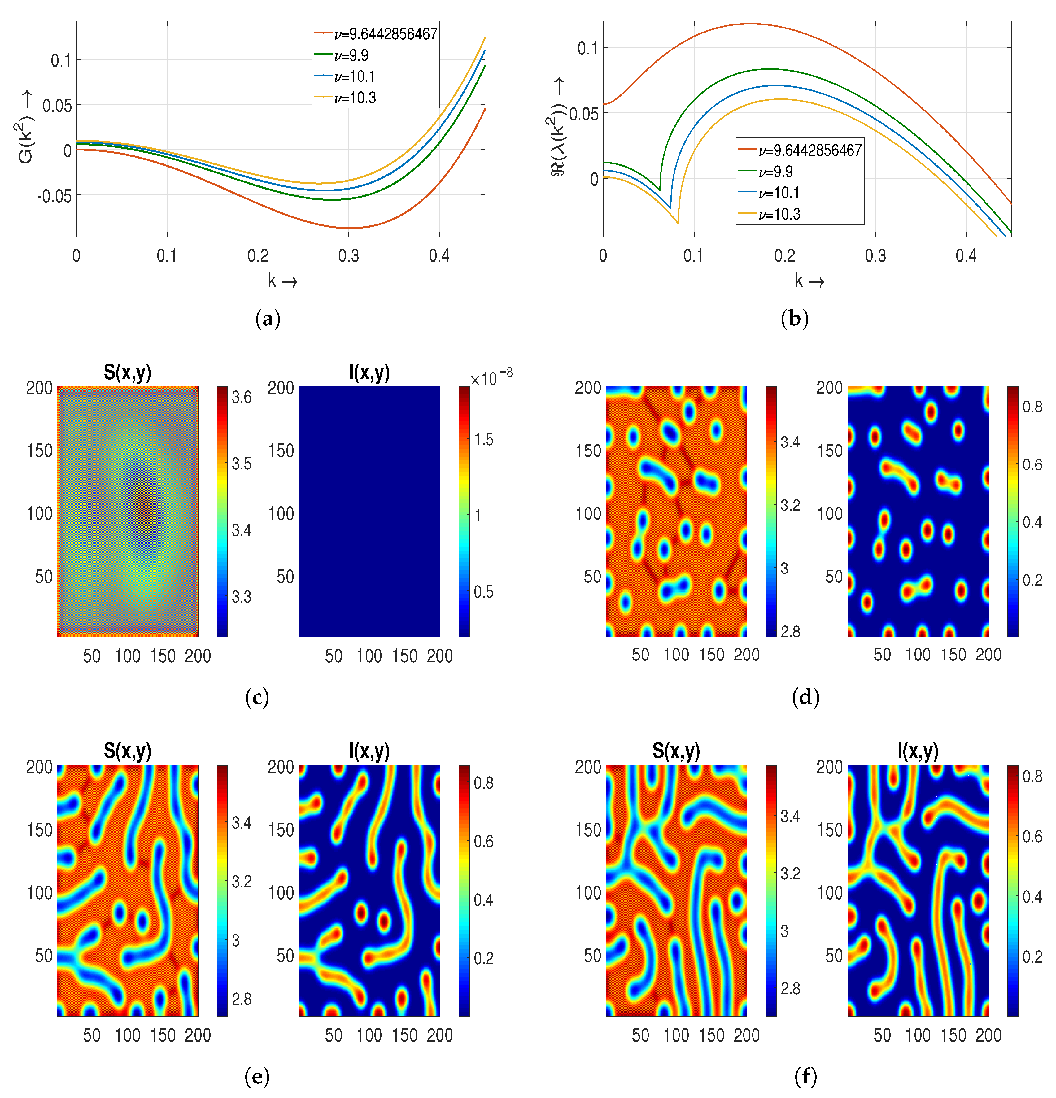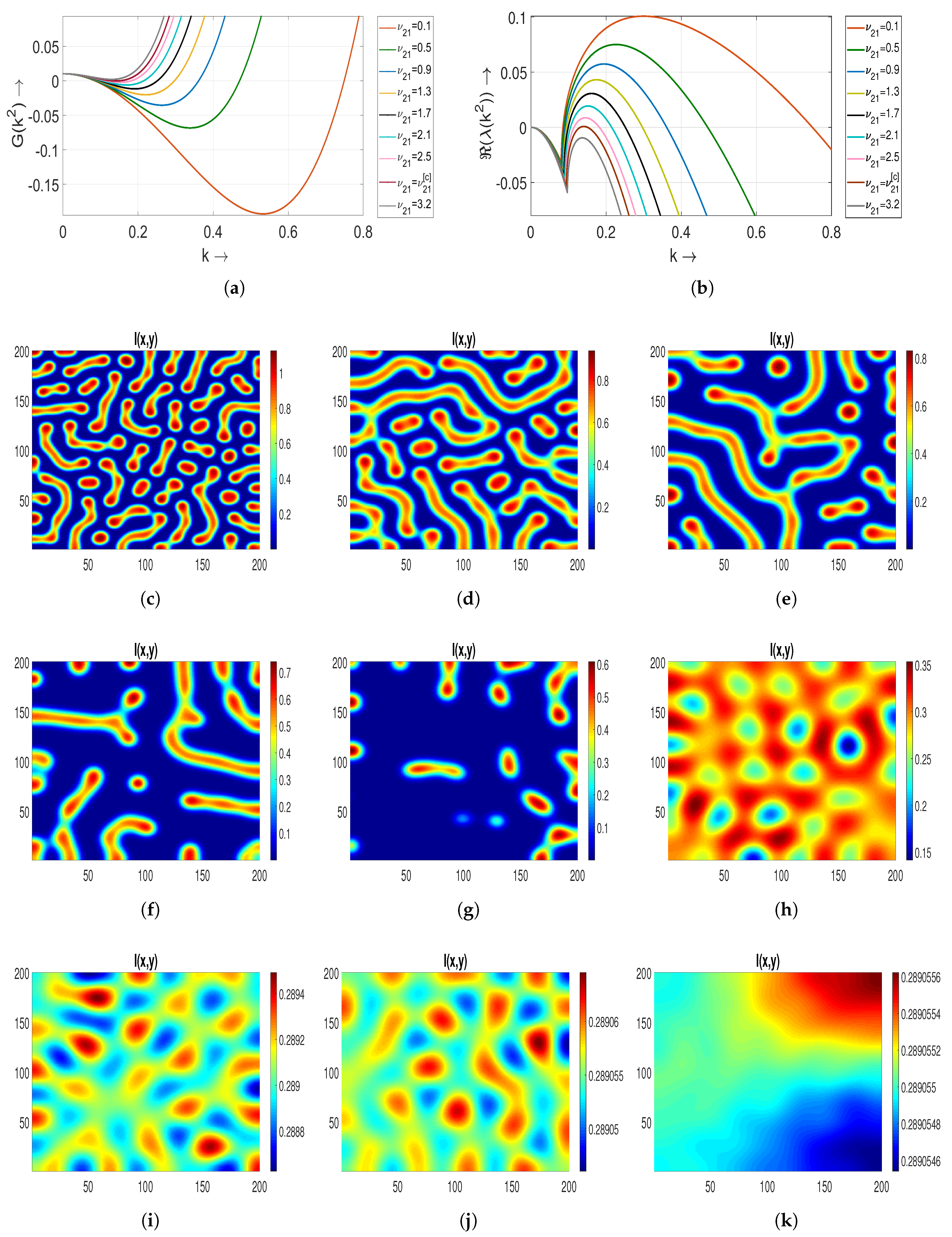For the diffusion coefficients mentioned in Table 2, it is clear from Figure 4a that the determinant of $J_S$ at the endemic state $E^{*}$ is negative. Also, the interval of wave number k, that is, $(-k^2,k^2)$ decreases as we increase $\nu$ in $(9.645,10.3389)$. In Figure 4b, we notice that the interval of a positive real part of the eigenvalues of $J_S$ also decreases with an increasing value of $\nu$. In Figure 4, we illustrated non-Turing patterns within the $R2$ region at time $t=500$. 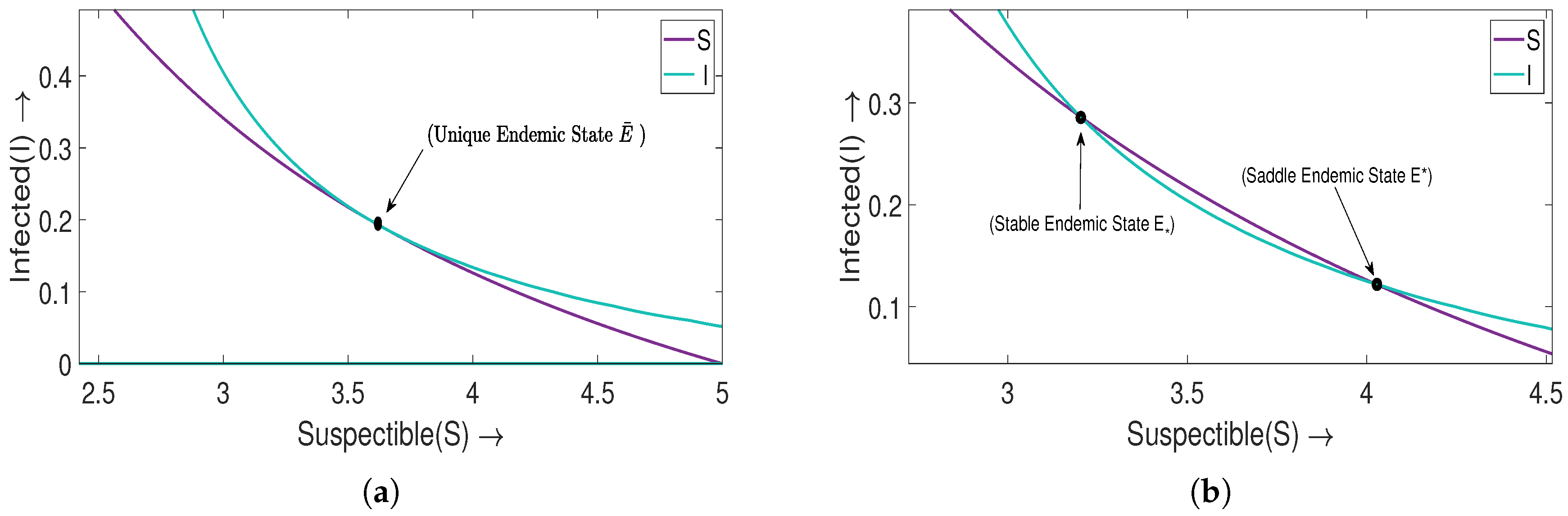In Figure 4c, a non-Turing pattern is observed for $\nu =9.6442856467$, where the two endemic states, $E^{*}$ and $E_{*}$, merge to form $\overline{E}$.

For $\nu =9.9$, high-density regions in the distribution of susceptible population manifest as blue holes against a reddish brown background of low density. Similarly, in the distribution of an infected population, red holes indicative of low density appear within a blue background, signifying a situation of heightened transmission [Figure 4d]. Moreover, as $\nu$ increases from $\nu =9.9$ to $10.1$, these individual holes coalesce, gradually giving rise to stripes. Consequently, a novel category of non-Turing patterns, characterized by a combination of strips and holes, emerges, as depicted in Figure 4e. Lastly, for $\nu =10.3$, Figure 4f portrays predominant strip-like non-Turing patterns. It is observed that, for the system (2), Hopf bifurcation occurs at $\nu =10.33894743$, and the equilibrium state $E^{*}$ starts to stabilize with further increments in the value of $\nu$. In the following subsection, we will proceed to investigate the Turing patterns.

5.2. Turing Patterns

Continuing from the preceding Section 5.1, we ascertain that the equilibrium state $E_{*}$ remains stable for $\nu \ge 10.33894743$. Furthermore, the condition for Turing instability persists within the same range of diffusion coefficients. Consequently, the resulting patterns in this scenario are classified as Turing patterns. We meticulously investigate these patterns across diverse values of the treatment parameter $\nu$ and the diffusion coefficient ${\alpha }_{21}$.

5.2.1. Effect of Treatment Parameter $\nu$ on Turing Patterns

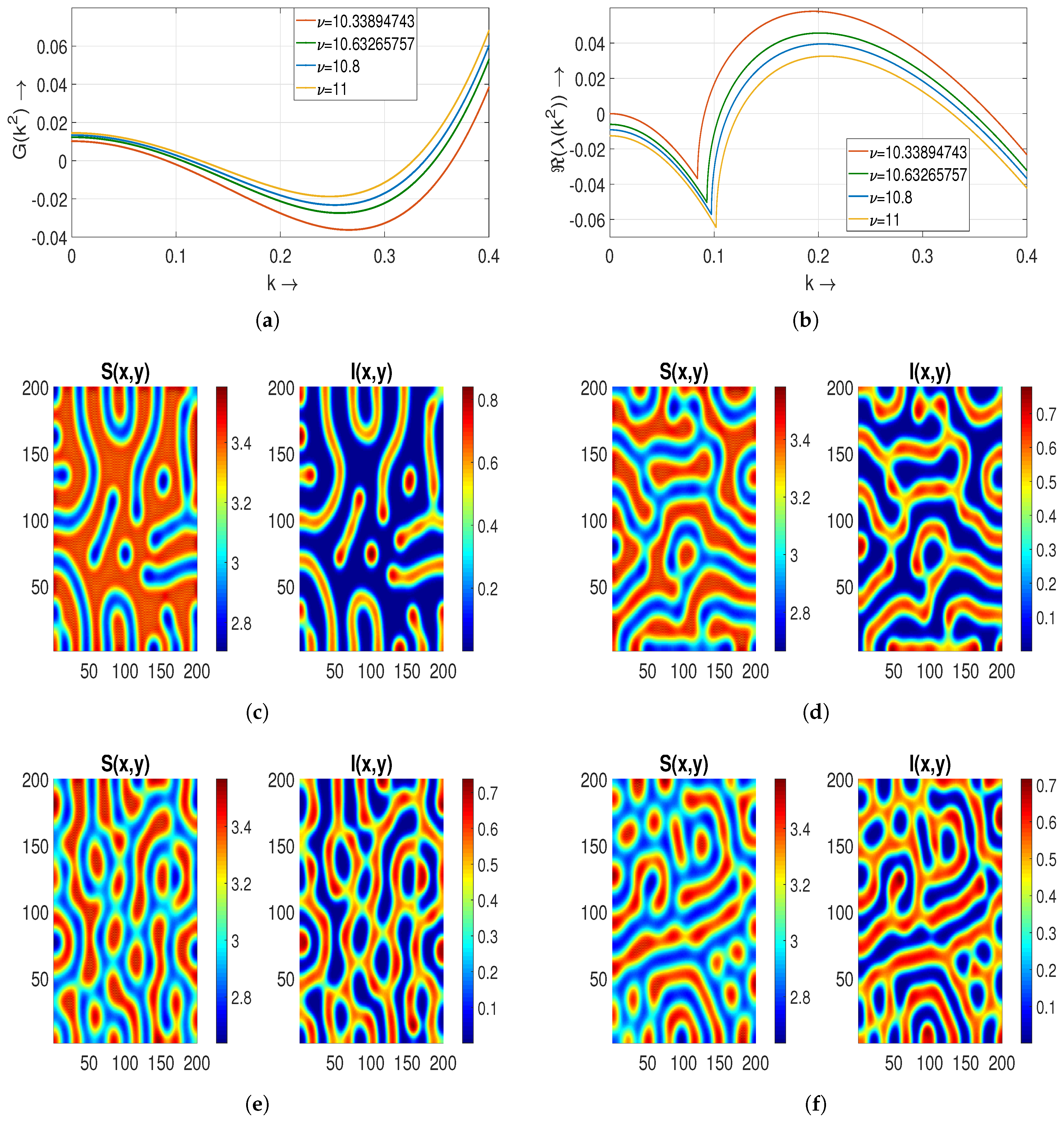
In Figure 5a,b, we plot $G\left(k^2\right)$ and $\Re \left(\lambda \left(k^2\right)\right)$ with respect to the wave number k to determine the Turing patterns at time $t=500$. It shows that the interval of $(-k^2,k^2)$ decreases as $\nu$ increases. As the equilibrium state $E^{*}$ is now stable and the conditions of Turing instability also hold, we obtain Turing patterns. Strips emerge with a blue color into the red background in Figure 5c,d for $\nu =10.33894743$ (corresponding to the Hopf bifurcation threshold) and $\nu =10.63265757$ in the distribution of the S individual. Meanwhile, in the distribution of I, we notice that red strips come out in the blue background. Hence, we conclude that the spread of a disease is high in this case. In order to determine the effect of saturation parameter $\nu$, we further choose two more values of $\nu$ as $\nu =10.8$ and $\nu =11$. For both the values of $\nu$, the roles of strips are now interchangeable in both cases compared to the above case. This results in the appearance of blue strips with a high-density region in a red background [Figure 5e,f].

5.2.2. Effect of Diffusion Coefficient ${\alpha }_{21}$ on Turing Patterns

For the numerical values of parameters given in Table 2, we determine the effect of the diffusion coefficient ${\alpha }_{21}$ on Turing patterns. Figure 6a,b show that the instability conditions hold. We observe that some holes are merging to form small strips, indicating a hole–strip mixed type pattern for ${\alpha }_{21}=0.1$ [Figure 6c].

For ${\alpha }_{21}=0.5$ and ${\alpha }_{21}=0.9$, in Figure 6d,e, it can be seen that these strips extend their size by mixing with holes, as well as strips. Thus, we obtain stripe-type patterns in which red strips with low-density regions appear in the blue background with high-density regions. Next, for ${\alpha }_{21}=1.3$, $1.7$, and $2.1$, we notice that these strips start disappearing in the form of a blue background and then come with dull holes in a red background. These dull blue holes with a high-density region come into the red background [Figure 6f–h]. This concludes that the region is safe for a certain time as the high-density region is small. Furthermore, for ${\alpha }_{21}=2.5$ and ${\alpha }_{21}={\alpha }_{21}^{\left[c\right]}=2.754624877$ (the numerical value of the Turing bifurcation threshold), these Turing patterns start to disappear as we get closer to the non-Turing patterns that we plot for ${\alpha }_{21}=3.2$ in Figure 6i–k. Here, Figure 6j represents a Turing–Hopf pattern.

5.3. Turing–Bogdanov–Takens Patterns

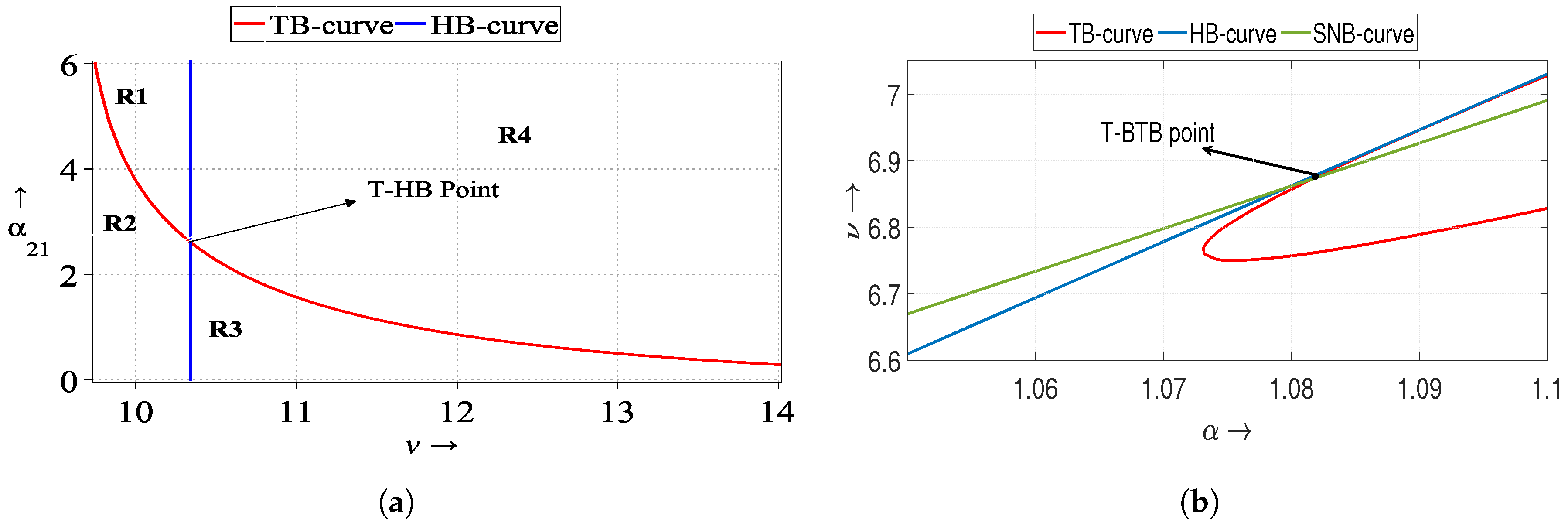
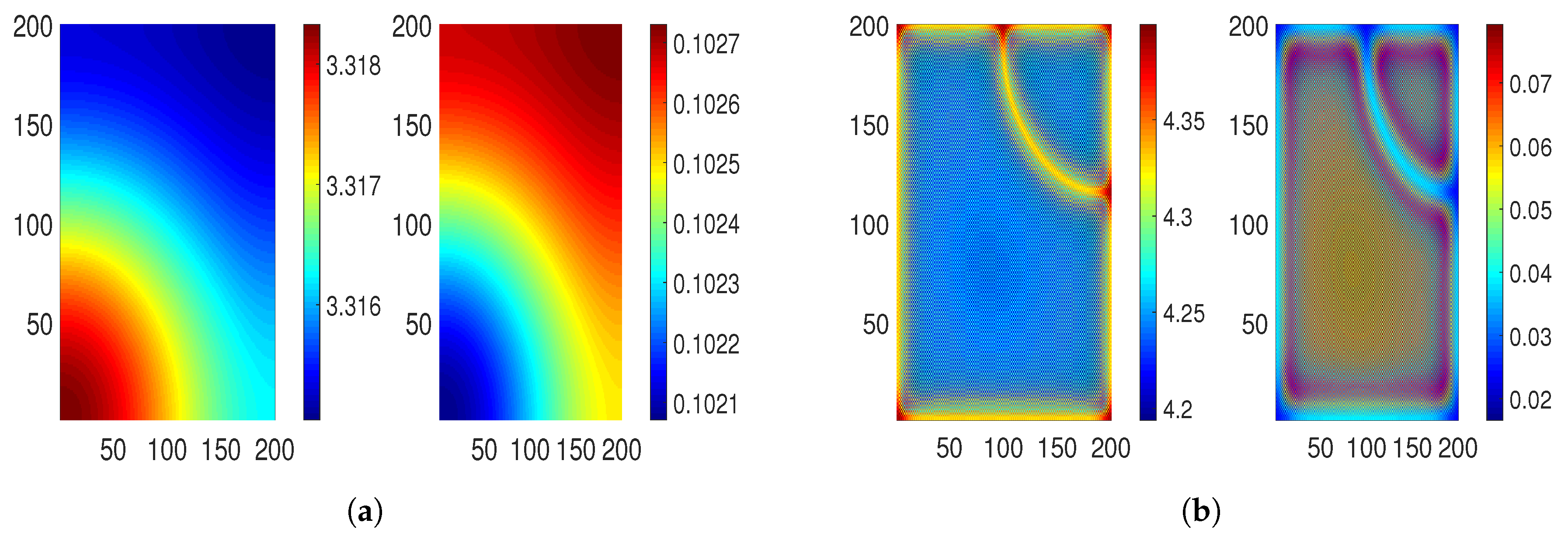
In the article [8], the authors explored the system (2) with parameter values $\Lambda =0.4$, $\delta =0.1$, $\beta =0.2$, $\mu =0.07$, and $ϵ=0.15$; the threshold values are $\alpha =0.66406412521$, $\nu =2.941192012$. Upon selecting specific diffusion coefficients in Table 3, the threshold value of the parameter ${\alpha }_{21}=9.327090512$, satisfied the conditions outlined in Remark 1 for the system (3). At the Turing–BT bifurcation, we obtained the pattern given in Figure 7a.

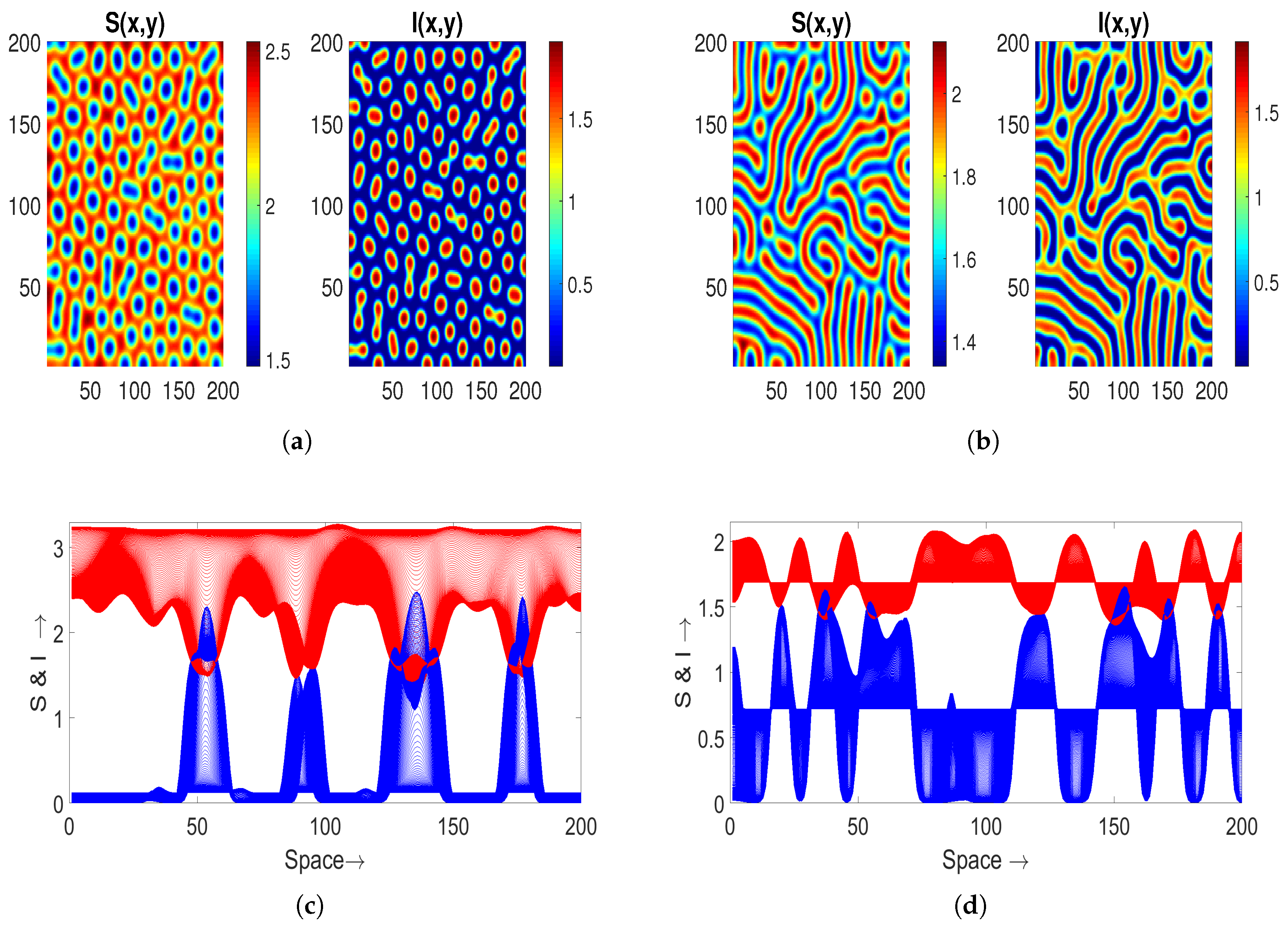
Further, with ${\alpha }_{21}=0.1,$ we observe Turing–Bogdanov–Takens patterns in Figure 8a. To examine the impact of treatment on the results, we increase the saturation factor $\nu$ in both cases: from $\nu =2.941192012$ to $\nu =4$. Notably, hole-type patterns manifest in Figure 8a, which subsequently converge into strips within the Turing space for $\nu =4$ (depicted in Figure 8b). The corresponding spatial series for both populations S (depicted in blue) and I (depicted in red), as illustrated in Figure 8c,d. These spatial series represent the associated 1D patterns.

To explore more about Turing–Bogdanov–Takens patterns, we take an alternative parameter set as $\Lambda =0.5$, $\delta =0.1$, $\beta =0.2$, $\mu =0.07$, $ϵ=0.4$, $\alpha =0.6230466144$, and $\nu =4.507073976$. 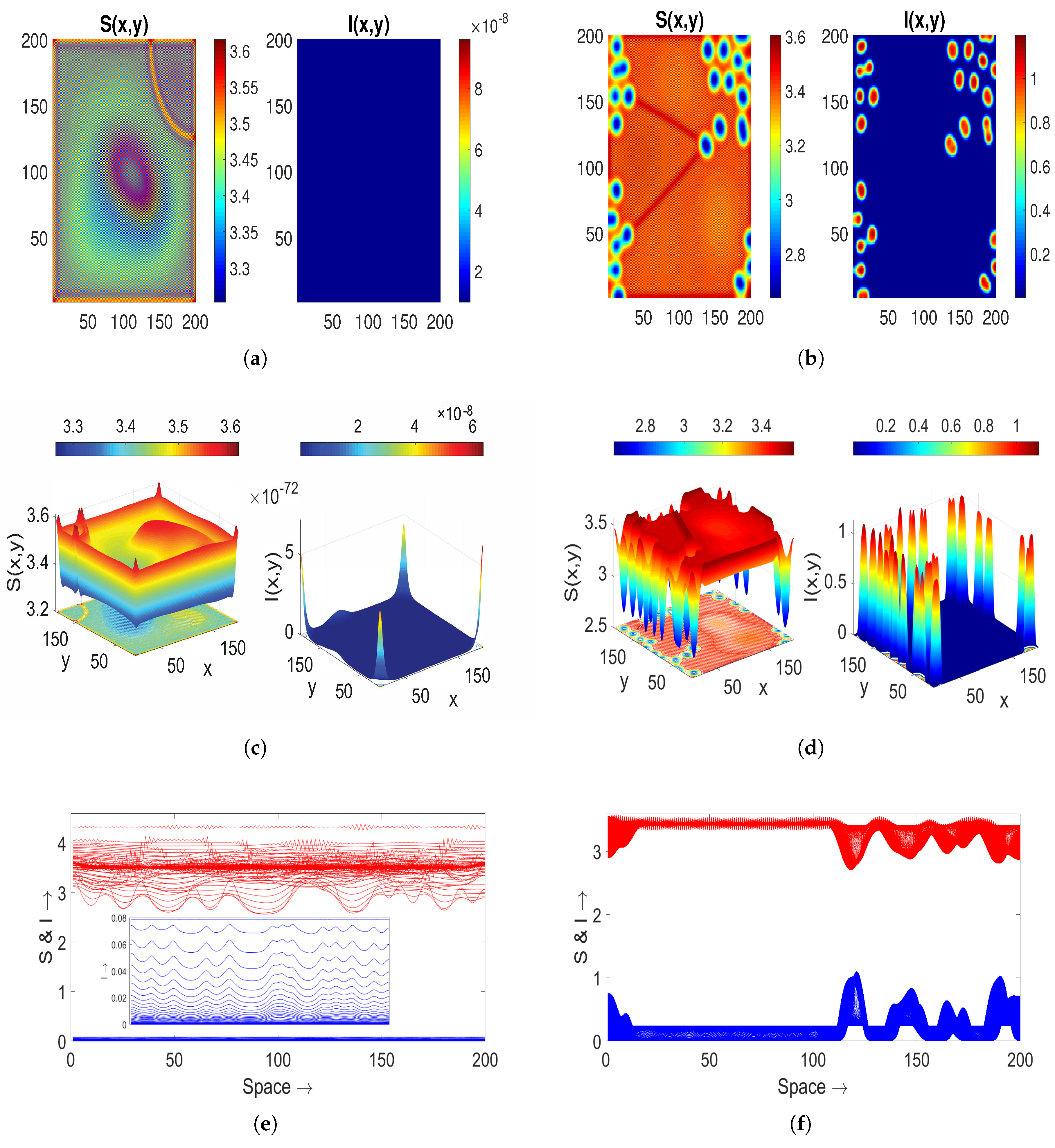With the diffusion coefficients mentioned in Table 3, we get the threshold value as ${\alpha }_{21}=12.34091682.$ Again, these parametric values verify the fulfillment of the Turing–Bogdanov–Takens condition discussed in Remark 1 around the endemic state $\overline{E}$, resulting in the jaggy pattern Figure 7b. If we choose the value of ${\alpha }_{21}=0.1$, then the disappearance of patterns is observed in Figure 9a. The extinction indicates the decline of the infected population, aligning with the outcomes of the corresponding ODE model (2), where solutions converge to the disease-free equilibrium state. In the scenario of increased saturation factor, $\nu =5.484$, hole-type Turing patterns reemerge in the distribution of both populations [Figure 9b]. Corresponding surfaces are depicted in Figure 9c,d, while spatial series are shown in Figure 9e,f.

5.4. Effect of Perturbation on the Evolution of Patterns

The dynamics of an epidemiological reaction–diffusion model are profoundly shaped by the initial values. Consequently, the emergence of patterns is substantially governed via the influence of perturbations. Recent works [41,47] portrayed patterns depicting the spread of a specific disease originating from a central focal point, highlighting the crucial role of the point of origin. 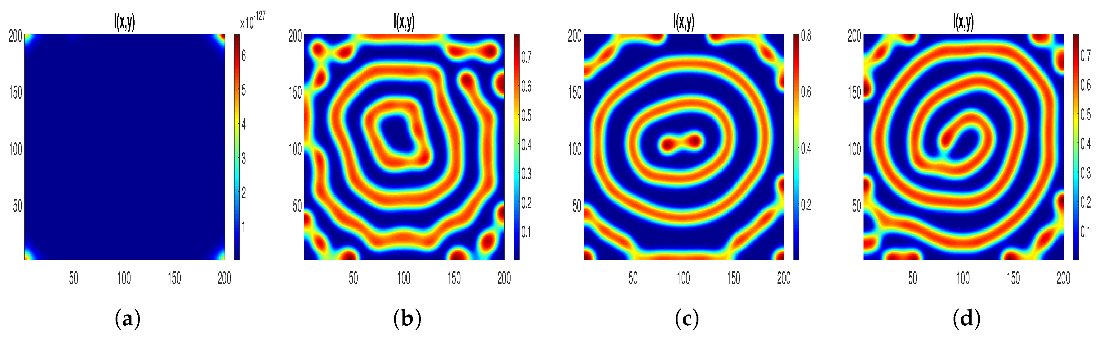In alignment with this observation, we are motivated to investigate the behavior of the system (3) under the same numerical parameter set as in the preceding scenarios. We aim to explore this behavior in the context of the introduced perturbation:

$$\begin{array}{c}\hfill {\mathbf{P}}_{\mathbf{2}}:\left\{\begin{array}{c}S(x,y)=S^{*}+3\times {10}^{-4}[{(x-100)}^2+{(y-100)}^2<200]\times randn,\hfill \\ I(x,y)=I^{*}+3\times {10}^{-4}[{(x-100)}^2+{(y-100)}^2<200]\times randn.\hfill \end{array}\right.\end{array}$$

For the parameters mentioned in Table 3, we present patterns with the ${\mathbf{P}}_{\mathbf{2}}$ perturbation in Figure 10. In order to comprehend the disease spread, our focus lies solely on the distribution of infected individuals. Notably, it is observed that low-density infected individuals are uniformly dispersed across the habitat, exhibiting blue coloration for $\nu =9.446$. This aligns with the extinction of the infected population, as indicated by the stability analysis of the disease-free state in the corresponding ODE system (2).

Furthermore, with increasing values of $\nu$, a noteworthy transition unfolds: regions with a high-density infected population (depicted in blue) start to emerge within different circles, while areas with a low-density infected population (depicted in red) begin to manifest against a blue background.

In Section 5.3, Turing–Bogdanov–Takens patterns were generated using three distinct sets of numerical parameters, along with the ${\mathbf{P}}_{\mathbf{1}}$ perturbation. In this section, we assess the resulting patterns under the same diffusion coefficient values for these parameter sets, this time introducing the ${\mathbf{P}}_{\mathbf{2}}$ perturbation. For the parameters $\Lambda =0.5$, $\delta =0.1$, $\beta =0.2$, $\mu =0.07$, $ϵ=0.4$, and $\alpha =0.62304661440$, we examine two values of the treatment parameter $\nu$ = $4.507073976$ and $\nu =5.484$. The resulting patterns are illustrated in Figure 11 at time $t=500$. These patterns indicate the formation of rings with varying radii in regions of low density. When the treatment parameter $\nu$ is altered, a disease initiates from the center of the disk and spreads across the entire area. Our analysis reveals that the distribution exhibits distinct zones of low and high infection, forming a striped pattern within a circular configuration. In conclusion, we infer that disease transmission is expected to be limited within this geographical area.

Table 2. Summary of patterns of Figure 4, Figure 5, Figure 6 and Figure 10. For biological parameters $\Lambda =0.5, ϵ=0.4, \alpha =0.9$ and $\delta =0.1, \beta =0.2, \mu =0.07$ and diffusion coefficients ${\delta }_{11}=0.6026, {\delta }_{12}=1.376, {\beta }_{11}=0.068, {\mu }_{11}=0.015, {ϵ}_{22}=0.014, {\delta }_{22}=0.08523, {\beta }_{22}=0.087, {\mu }_{22}=0.181, {\alpha }_{22}=0.145$.

Sr. No.	Parameter Values	Nature of ${\mathit{E}}^{*}$	Type of Patterns	Figure
$1\left(i\right)$	${\alpha }_{21}=0.884$, $\nu =9.6442856467,$ and $\nu =9.9$	Unstable	Non-Turing	With ${\mathbf{P}}_{\mathbf{1}}$-Figure 4c,d and with ${\mathbf{P}}_{\mathbf{2}}$-Figure 10a,b
$1\left(ii\right)$	${\alpha }_{21}=0.884$, $\nu =10.1$ and $\nu =10.3$	Unstable	Non-Turing	With ${\mathbf{P}}_{\mathbf{1}}$-Figure 4e,f
$1\left(iii\right)$	${\alpha }_{21}=0.884$, $\nu =10.33894743,$$\nu =10.63$	Stable	Turing	With ${\mathbf{P}}_{\mathbf{1}}$-Figure 5c,d and with ${\mathbf{P}}_{\mathbf{2}}$-Figure 10c,d
$1\left(iv\right)$	${\alpha }_{21}=0.884$, $\nu =10.8$ and $\nu =11$	Stable	Turing	With ${\mathbf{P}}_{\mathbf{1}}$-Figure 5e,f
$2\left(i\right)$	$\nu =10.33894743$, ${\alpha }_{21}=0.1,0.5,0.9,1.3,1.7,2.1,2.5$	Stable	Turing	With ${\mathbf{P}}_{\mathbf{1}}$-Figure 6c–i
$2\left(ii\right)$	$\nu =10.33894743$, ${\alpha }_{21}^{\left[c\right]}=2.754624877$	Non-hyperbolic	Turing–Hopf	With ${\mathbf{P}}_{\mathbf{1}}$-Figure 6j
$2\left(iii\right)$	$\nu =10.33894743$, ${\alpha }_{21}=3.2$	Stable	Non-Turing	With ${\mathbf{P}}_{\mathbf{1}}$-Figure 6k

Table 2. Summary of patterns of Figure 4, Figure 5, Figure 6 and Figure 10. For biological parameters $\Lambda =0.5, ϵ=0.4, \alpha =0.9$ and $\delta =0.1, \beta =0.2, \mu =0.07$ and diffusion coefficients ${\delta }_{11}=0.6026, {\delta }_{12}=1.376, {\beta }_{11}=0.068, {\mu }_{11}=0.015, {ϵ}_{22}=0.014, {\delta }_{22}=0.08523, {\beta }_{22}=0.087, {\mu }_{22}=0.181, {\alpha }_{22}=0.145$.

Sr. No.	Parameter Values	Nature of ${\mathit{E}}^{*}$	Type of Patterns	Figure
$1\left(i\right)$	${\alpha }_{21}=0.884$, $\nu =9.6442856467,$ and $\nu =9.9$	Unstable	Non-Turing	With ${\mathbf{P}}_{\mathbf{1}}$-Figure 4c,d and with ${\mathbf{P}}_{\mathbf{2}}$-Figure 10a,b
$1\left(ii\right)$	${\alpha }_{21}=0.884$, $\nu =10.1$ and $\nu =10.3$	Unstable	Non-Turing	With ${\mathbf{P}}_{\mathbf{1}}$-Figure 4e,f
$1\left(iii\right)$	${\alpha }_{21}=0.884$, $\nu =10.33894743,$$\nu =10.63$	Stable	Turing	With ${\mathbf{P}}_{\mathbf{1}}$-Figure 5c,d and with ${\mathbf{P}}_{\mathbf{2}}$-Figure 10c,d
$1\left(iv\right)$	${\alpha }_{21}=0.884$, $\nu =10.8$ and $\nu =11$	Stable	Turing	With ${\mathbf{P}}_{\mathbf{1}}$-Figure 5e,f
$2\left(i\right)$	$\nu =10.33894743$, ${\alpha }_{21}=0.1,0.5,0.9,1.3,1.7,2.1,2.5$	Stable	Turing	With ${\mathbf{P}}_{\mathbf{1}}$-Figure 6c–i
$2\left(ii\right)$	$\nu =10.33894743$, ${\alpha }_{21}^{\left[c\right]}=2.754624877$	Non-hyperbolic	Turing–Hopf	With ${\mathbf{P}}_{\mathbf{1}}$-Figure 6j
$2\left(iii\right)$	$\nu =10.33894743$, ${\alpha }_{21}=3.2$	Stable	Non-Turing	With ${\mathbf{P}}_{\mathbf{1}}$-Figure 6k

Table 3. Summary of patterns of Figure 8, Figure 9 and Figure 11. We fixed biological constants as $\delta =0.1, \beta =0.2, \mu =0.07$ and the diffusion coefficients as ${\delta }_{11}=0.6026, {\delta }_{12}=1.376, {\beta }_{11}=0.068, {\mu }_{11}=0.015, {ϵ}_{22}=0.014, {\delta }_{22}=0.08523, {\beta }_{22}=0.087$, ${\mu }_{22}=0.181, {\alpha }_{21}=0.01, {\alpha }_{22}=0.05$. Here, BT = Bogdanov–Takens, and ${\mathbf{P}}_{\mathbf{1}}$, ${\mathbf{P}}_{\mathbf{2}}$ = perturbation.

Sr. No.	Parameter Values	Nature of ${\mathit{E}}^{*}$	Type of Patterns	Figure
$1\left(i\right)$	$\Lambda =0.4, ϵ=0.15, \alpha =0.66406412521,$$\nu =2.941192012$	double-zero equilibrium	Turing-B-T	With ${\mathbf{P}}_{\mathbf{1}}$-Figure 8a,c
$1\left(ii\right)$	$\Lambda =0.4, ϵ=0.15, \alpha =0.66406412521,$$\nu =4$	Stable	Turing	With ${\mathbf{P}}_{\mathbf{1}}$-Figure 8b,d
$2\left(i\right)$	$\Lambda =0.5, ϵ=0.4, \alpha =0.6230466144,$$\nu =4.507073976$	double-zero equilibrium	Turing-B-T	With ${\mathbf{P}}_{\mathbf{1}}$-Figure 9c,e and with ${\mathbf{P}}_{\mathbf{2}}$-Figure 11a
$2\left(ii\right)$	$\Lambda =0.5, ϵ=0.4, \alpha =0.6230466144,$$\nu =5.484$	Stable	Turing	With ${\mathbf{P}}_{\mathbf{1}}$-Figure 9d,f and with ${\mathbf{P}}_{\mathbf{2}}$-Figure 11c

Table 3. Summary of patterns of Figure 8, Figure 9 and Figure 11. We fixed biological constants as $\delta =0.1, \beta =0.2, \mu =0.07$ and the diffusion coefficients as ${\delta }_{11}=0.6026, {\delta }_{12}=1.376, {\beta }_{11}=0.068, {\mu }_{11}=0.015, {ϵ}_{22}=0.014, {\delta }_{22}=0.08523, {\beta }_{22}=0.087$, ${\mu }_{22}=0.181, {\alpha }_{21}=0.01, {\alpha }_{22}=0.05$. Here, BT = Bogdanov–Takens, and ${\mathbf{P}}_{\mathbf{1}}$, ${\mathbf{P}}_{\mathbf{2}}$ = perturbation.

Sr. No.	Parameter Values	Nature of ${\mathit{E}}^{*}$	Type of Patterns	Figure
$1\left(i\right)$	$\Lambda =0.4, ϵ=0.15, \alpha =0.66406412521,$$\nu =2.941192012$	double-zero equilibrium	Turing-B-T	With ${\mathbf{P}}_{\mathbf{1}}$-Figure 8a,c
$1\left(ii\right)$	$\Lambda =0.4, ϵ=0.15, \alpha =0.66406412521,$$\nu =4$	Stable	Turing	With ${\mathbf{P}}_{\mathbf{1}}$-Figure 8b,d
$2\left(i\right)$	$\Lambda =0.5, ϵ=0.4, \alpha =0.6230466144,$$\nu =4.507073976$	double-zero equilibrium	Turing-B-T	With ${\mathbf{P}}_{\mathbf{1}}$-Figure 9c,e and with ${\mathbf{P}}_{\mathbf{2}}$-Figure 11a
$2\left(ii\right)$	$\Lambda =0.5, ϵ=0.4, \alpha =0.6230466144,$$\nu =5.484$	Stable	Turing	With ${\mathbf{P}}_{\mathbf{1}}$-Figure 9d,f and with ${\mathbf{P}}_{\mathbf{2}}$-Figure 11c

6. Conclusions

In reality, an individual’s movement is influenced by a multitude of factors, including their disease-related precautions, access to medical care, and various other considerations. In light of these factors, we propose and employ a novel nonlinear cross-diffusion approach to investigate an SIR epidemic model featuring saturated-type treatment. Our proposed cross-diffusion mechanism, characterized by a combination of quadratic and rational components, offers enhanced realism compared to existing formulations in the literature. Importantly, the accuracy of this cross-diffusion representation is demonstrated concerning the populations’ mobility capacity through flux calculations. Utilizing coupled upper and lower solutions for elliptic partial differential equations, we establish the admissibility of at least one non-constant endemic state within the reduced SIR model augmented with the proposed cross-diffusion. This finding underscores the potential coexistence of susceptible and infected populations within their environment. To illustrate potential pattern formation scenarios driven by Turing instability, we numerically simulate the proposed model in a square environment of dimensions $200\times 200$.

We modulate the treatment parameter $\nu$ to assess the impact of delaying treatment for infected individuals. We acknowledge the potential for a significant influence on pattern evolution based on variations in the initial disturbance. Therefore, in this study, we propose two novel perturbations, denoted as ${\mathbf{P}}_{\mathbf{1}}$ and ${\mathbf{P}}_{\mathbf{2}}$, to explore diverse pattern types. We observe that, when the parameters associated with temporal models and diffusion coefficients are modified using the first perturbation ${\mathbf{P}}_{\mathbf{1}}$, patterns such as holes, strips, and mixture-type patterns emerge. However, it is noteworthy that patterns obtained with the ${\mathbf{P}}_{\mathbf{1}}$ perturbation transition into circular strips under ${\mathbf{P}}_{\mathbf{2}}$. This observation illustrates how a disease can propagate in the form of concentric stripe rings of varying radii when originating from a specific point, the disease’s center of origin. Additionally, through the identification of codimension-2 Turing–Hopf bifurcation, we determine the Turing space.

The authors [8] investigate the existence of two pairs of Bogdanov–Takens bifurcation thresholds in the corresponding temporal model. For these parameter sets, a specific combination of diffusion coefficients is selected to observe Turing–Bogdanov–Takens patterns with both perturbations. It is observed that distinct patterns emerge for these parameter sets, and contrary to temporal predictions, the infection persists within the system. Consequently, a new set of relevant parameters is considered. It is concluded that, for lower values of $\nu$ (which measures the delay in treatment for the infected population), the infected population becomes extinct due to the absence of a stable endemic state in the corresponding ODE model. This aligns with equilibrium stability results, where solutions converge towards the disease-free equilibrium state. Additionally, various non-Turing patterns around the unstable equilibrium state are plotted, meeting the criteria for Turing instability for different $\nu$ values. When two endemic states are present, directed patterns suffer more significant disruption than in the case of a single endemic state. This implies that disease transmission worsens with increasing $\nu$ values. The impact of the diffusion coefficient ${\alpha }_{21}$ is examined through numerical simulations to understand the influence of the suggested cross-diffusion. This work represents a modest advancement in comprehending the role of movement for both susceptible and infected populations in infectious disease modeling.

Model Limitations and Applicability: While this study highlights the influence of cross-diffusion and spatial heterogeneity under movement-restricted settings, its applicability to highly mobile populations—such as during the COVID-19 pandemic—is limited. The zero-flux boundary assumption does not reflect real-world mobility enabled by transportation networks like airports and highways. Moreover, the model assumes symptomatic transmission, which fails to capture diseases with significant asymptomatic or pre-symptomatic spread, such as COVID-19. In such cases, avoidance behavior is ineffective since infected individuals are not easily identifiable. To address these limitations, future work could incorporate nonlocal dispersal, mobility networks, and additional compartments for asymptomatic or undetected carriers to better reflect real-world transmission dynamics.