Reducing the Primary Resonance Vibrations of a Cantilever Beam Using a Proportional Fractional-Order Derivative Controller

Abstract

Many studies aim to suppress vibrations in vibrating dynamic systems, such as bridges, highways, and aircraft. In this study, we scrutinize the primary resonance of a cantilever beam excited by an external force via a proportional fractional-order derivative controller (PFD). The average method is used to obtain the approximate solution of the vibrating system. The stability of the control system is illustrated using the Routh–Hurwitz criterion. We investigate the performance of some chosen parameters of the studied system to generate response curves. The performance of the linear fractional feedback control is studied at different values of the fractional order.

1. Introduction

Many types of controllers are used for suppressing the vibrations of different nonlinear dynamic systems, such as negative linear velocity feedback, negative cubic velocity feedback, nonlinear saturation controllers (NSCs), nonlinear integral positive position feedback controllers (NIPPFs), integral resonant controllers (IRCs), negative derivative feedback controllers (NDFs), and time delay control. Multiple time scales have been used to investigate microbeams’ nonlinear vibrations for two different resonance cases (super-harmonic and harmonic resonances). From this investigation, it was found that the boundary conditions affect the microbeams’ vibrations [1]. Recently, the vibrations of many vibrating systems [2,3,4,5,6,7,8] have been suppressed using different types of control. Fractional calculus is one of the most important research areas in this field, attracting many researchers in science and engineering [9,10,11]. A proportional–derivative (PD) controller is often employed to regulate oscillations by adjusting the system’s response to disturbances. Refs. [12,13,14,15] presented a new control strategy combining PD controllers, IRCs, and PPF controllers to reduce vibrations in eight- and twelve-pole electromagnetic suspension systems. The systems’ dynamics were framed as a nonlinear four-degree-of-freedom system, and the effectiveness of different control strategies was scrutinized. The results clarified that the combined PD + IRC + PPF controller successfully eliminated vibrations under various conditions, offering the benefits of the individual controllers without their drawbacks. Abd El-Salam et al. [16] examined and solved a system of nonlinear differential equations constituting the oscillations of a cantilever beam, using PD and NDF controllers to reduce vibrations. Their study scrutinized the frequency response curves, comparing the controllers and evaluating their effects on the stability and response curves under different resonance cases. Ibrahim [17] focused on tuning PI-PD controllers, an extension of PID controllers, to stabilize open-loop unstable processes by using a PD controller in an inner feedback loop. He derived the tuning parameters using analytical rules based on the integral of the squared time-cubed error (IST3E) criterion, and simulations demonstrated the effectiveness and superiority of the proposed approach. In the field of control, fractional order has been used as a tool for suppressing the vibrations of many dynamic systems. A linear single-degree-of-freedom oscillator was investigated by Wang, Hu, and Du [18,19] with a fractional-order derivative. Leung et al. [20] proposed a generalized Duffing–van der Pol oscillator:

$$u^{″}-\hspace{0.17em}{D}_t^{\lambda }\hspace{0.17em}\left(\alpha \hspace{0.17em}u-\beta \hspace{0.17em}{u}^3\right)+k_0\hspace{0.17em}u+k_3\hspace{0.17em}{u}^3=0$$

(1)

where the cubic displacement involved in the fractional operator is used to describe the nonlinear damping of order $\lambda$ ($0<\lambda <1$). To solve the fractional van der Pol oscillator analytically, the residue harmonic balance method was proposed by Leung et al. in [21,22]. Xie and Lin [23] used the two-scale expansion method to illustrate the dynamic behavior of a small-damped fractional system. The unforced fractional van der Pol oscillator, presented as

$$\hspace{0.17em}{D}_t^{1+\lambda }\hspace{0.17em}u-\epsilon \left(1-u^2\right)D_t^{\lambda }\hspace{0.17em}u+\hspace{0.17em}u=0,$$

(2)

was studied by Barbosa et al. [24]. They stated that the fractional order can act as a modulation parameter that may be useful for a better understanding and control of the standard van der Pol oscillator. Zhoujin [25] investigated the primary resonance and feedback control of the fractional Duffing–van der Pol oscillator with a quantic nonlinear restoring force, which is given by a second-order non-autonomous differential equation, as follows:

$$\ddot{x}-\mu \left(1-x^2\right)D_t^{q}x+\alpha x+\lambda x^3+\beta x^5=f\hspace{0.17em}\cos \omega t0<q\le 1$$

(3)

He stated that larger fractional orders and larger damping coefficients can reduce the effective amplitude of resonance and change the resonance frequency. The fractional derivative has been used to improve the performance of many dynamic systems [26,27,28,29,30].

This article will explore the use of a proportional fractional-order derivative controller to control the primary resonance of a cantilever beam excited by an external force. Through theoretical analysis and simulation, the effectiveness of the PFD controller in handling two types of oscillators is evaluated, providing insights into its application in real-world systems.

2. Mathematical Treatment

In mechanics, a cantilever beam is a structural element that is fixed at one end and free at the other, as shown in Figure 1.

The equation of motion of a cantilever beam is given by a one-degree-of-freedom second-order differential equation, as follows:

$$\ddot{x}+{\omega }^2\hspace{0.17em}x+{\gamma }_1\hspace{0.17em}{x}^3+\zeta \hspace{0.17em}\dot{\mathrm{x}}+{\gamma }_2\hspace{0.17em}{\dot{x}}^3+\beta \hspace{0.17em}\left(x\hspace{0.17em}{\dot{x}}^2+x^2\hspace{0.17em}\ddot{x}\right)=f\hspace{0.17em}\cos (\mathrm{\Omega }\hspace{0.17em}\mathrm{t})+F_c(t)$$

(4)

where $x$ is the displacement of the cantilever beam and its natural frequency is $\omega$; the damping coefficient is $\zeta$; the coefficients of the nonlinearity terms are $\beta$ and ${\gamma }_j\hspace{0.17em}(j=1,2)$; and the excitation frequency and amplitude are $\mathrm{\Omega }$ and $f$. To suppress the vibrations of the cantilever beam, we utilized proportional fractional-order derivative feedback control, as shown in the closed loop in Figure 2. The control feedback signal $F_c(t)$ takes the form

$$F_c(t)=-K_1\hspace{0.17em}x(t)-K_2\hspace{0.17em}{D}_t^{\alpha }\left\{x(t)\right\}$$

(5)

where $0\le \alpha \le 1$, $K_1$ is the proportional feedback gain, and $K_2$ is the fractional-order derivative controller feedback gain. According to Caputo’s definition [26],

$$D_t^{\alpha }\left\{x(t)\right\}=\left\{\begin{array}{l}{\displaystyle \frac{1}{\mathsf{\Gamma }(1-\alpha )}}\hspace{0.17em}{\displaystyle \underset{0}{\overset{t}{\int }}\frac{x^{\prime }(\tau )}{{(t-\tau )}^{\alpha }}}\hspace{0.17em}d\tau \\ {\displaystyle \frac{dx}{dt}},\hspace{0.17em}\hspace{0.17em}\hspace{0.17em}\hspace{0.17em}\hspace{0.17em}\hspace{0.17em}\hspace{0.17em}\hspace{0.17em}for\hspace{0.17em}\hspace{0.17em}\hspace{0.17em}\hspace{0.17em}\alpha =1\end{array}\right.$$

(6)

For the primary resonance case, we use the average method, as follows:

$${\mathsf{\Omega }}^2={\omega }^2+\sigma$$

(7)

Relying on the average method, the approximate solution for the cantilever beam equation of motion can be written as follows [27]:

$$x(\mathrm{t})=\mathrm{a}\hspace{0.17em}\cos \varphi ;\hspace{0.17em}\hspace{0.17em}\hspace{0.17em}\hspace{0.17em}\hspace{0.17em}\hspace{0.17em}\hspace{0.17em}\hspace{0.17em}\hspace{0.17em}\hspace{0.17em}\hspace{0.17em}\hspace{0.17em}\varphi =\mathsf{\Omega }\mathrm{t}+\theta$$

(8a)

$$\dot{x}(\mathrm{t})=-\mathrm{a}\mathsf{\Omega }\hspace{0.17em}\sin \varphi$$

(8b)

$$\ddot{x}(\mathrm{t})=-\mathrm{a}{\mathsf{\Omega }}^2\hspace{0.17em}\cos \varphi$$

(8c)

where $a,\hspace{0.17em}\hspace{0.17em}\hspace{0.17em}\varphi$ are the amplitude and the generalized phase. Now, by differentiating Equation (8a) with respect to t,

$$\dot{x}(\mathrm{t})=\dot{a}\hspace{0.17em}\cos \varphi -a\dot{\theta }\sin \varphi -\mathrm{a}\mathsf{\Omega }\sin \varphi$$

(9)

Comparing Equations (8b) and (9), we get

$$\dot{a}\hspace{0.17em}\cos \varphi -a\dot{\theta }\sin \varphi =0$$

(10)

The second derivative of $x(t)$ from Equation (8b) concerning t is given by

$$\ddot{x}(\mathrm{t})=-\mathsf{\Omega }\dot{a}\hspace{0.17em}\sin \varphi -a\mathsf{\Omega }\dot{\theta }\cos \varphi -\mathrm{a}{\mathsf{\Omega }}^2\cos \varphi$$

(11)

$$\ddot{x}(\mathrm{t})+{\mathsf{\Omega }}^{2}x=-\mathsf{\Omega }\left(\dot{a}\hspace{0.17em}\sin \varphi +a\dot{\theta }\cos \varphi \right)$$

(12)

From Equation (4), we get the following:

$$\ddot{x}(\mathrm{t})+{\mathsf{\Omega }}^{2}x=f\hspace{0.17em}\cos (\mathsf{\Omega }\hspace{0.17em}\mathrm{t})+\mathrm{\sigma }\hspace{0.17em}\mathrm{x}-{\gamma }_1\hspace{0.17em}{x}^3-\zeta \hspace{0.17em}\dot{\mathrm{x}}-{\gamma }_2\hspace{0.17em}{\dot{x}}^3-\beta \hspace{0.17em}\left(x\hspace{0.17em}{\dot{x}}^2+x^2\hspace{0.17em}\ddot{x}\right)-K_1\hspace{0.17em}x-K_2\hspace{0.17em}{D}_t^{\alpha }\left\{x(t)\right\}$$

(13)

From Equations (12) and (13), we get the following equation:

$$\dot{a}\hspace{0.17em}\sin \varphi +a\dot{\theta }\cos \varphi =-{\displaystyle \frac{1}{\mathsf{\Omega }}}\left(f\hspace{0.17em}\cos (\mathsf{\Omega }\hspace{0.17em}\mathrm{t})+\mathsf{\sigma }\hspace{0.17em}\mathrm{x}-{\gamma }_1\hspace{0.17em}{x}^3-\zeta \mathsf{\hspace{0.17em}}\dot{x}-{\gamma }_2\hspace{0.17em}{\dot{x}}^3-\beta \hspace{0.17em}\left(x\hspace{0.17em}{\dot{x}}^2+x^2\hspace{0.17em}\ddot{x}\right)-K_1\hspace{0.17em}x-K_2\hspace{0.17em}{D}_t^{\alpha }\left\{x(t)\right\}\right)$$

(14)

To simplify Equation (14), we will write it as

$$\dot{a}\hspace{0.17em}\sin \varphi +a\dot{\theta }\cos \varphi =-{\displaystyle \frac{1}{\mathsf{\Omega }}}\left(P_1(a,\theta )+P_2(a,\theta )\right)$$

(15)

where

$P_1(a,\theta )=f\hspace{0.17em}\cos (\mathsf{\Omega }\hspace{0.17em}\mathrm{t})+\mathsf{\sigma }\hspace{0.17em}\mathrm{x}-{\gamma }_1\hspace{0.17em}{x}^3-\zeta \mathsf{\hspace{0.17em}}\dot{\mathrm{x}}-{\gamma }_2\hspace{0.17em}{\dot{x}}^3-\beta \hspace{0.17em}\left(x\hspace{0.17em}{\dot{x}}^2+x^2\hspace{0.17em}\ddot{x}\right)-K_1\hspace{0.17em}x$ and $P_2(a,\theta )=-k_2\hspace{0.17em}{D}_t^{\alpha }\left\{x(t)\right\}$. The use of Equation (8) leads to

$$\begin{array}{l}{P}_1(a,\theta )=f\hspace{0.17em}\cos (\varphi -\theta )+\mathsf{\sigma }\hspace{0.17em}a\hspace{0.17em}\cos \varphi -{\gamma }_1\hspace{0.17em}{(a\cos \varphi )}^3+\mathsf{\Omega }\hspace{0.17em}\zeta \hspace{0.17em}a\sin \varphi +{\gamma }_2{\mathsf{\Omega }}^3\hspace{0.17em}{(a\sin \varphi )}^3-\beta \hspace{0.17em}{\mathsf{\Omega }}^2{a}^3{(\sin \varphi )}^2\cos \varphi \\ \hspace{0.17em}\hspace{0.17em}\hspace{0.17em}\hspace{0.17em}\hspace{0.17em}\hspace{0.17em}\hspace{0.17em}\hspace{0.17em}\hspace{0.17em}\hspace{0.17em}\hspace{0.17em}\hspace{0.17em}\hspace{0.17em}\hspace{0.17em}\hspace{0.17em}\hspace{0.17em}\hspace{0.17em}\hspace{0.17em}\hspace{0.17em}+\beta \hspace{0.17em}{\mathsf{\Omega }}^2{a}^3{(\cos \varphi )}^3-K_1\hspace{0.17em}a\hspace{0.17em}\cos \varphi \end{array}$$

(16)

From Equations (10) and (15),

$$\dot{a}\hspace{0.17em}=-{\displaystyle \frac{1}{\mathsf{\Omega }}}\left(P_1(a,\theta )+P_2(a,\theta )\right)\hspace{0.17em}\sin \varphi$$

(17)

$$a\dot{\theta }=-{\displaystyle \frac{1}{\mathsf{\Omega }}}\left(P_1(a,\theta )+P_2(a,\theta )\right)\hspace{0.17em}\cos \varphi$$

(18)

Moreover, one could apply the standard averaging method for Equations (17) and (18) in the interval [0, T].

$$\dot{a}\hspace{0.17em}=-{\displaystyle \frac{1}{\mathsf{\Omega }\hspace{0.17em}T}}{\displaystyle \underset{0}{\overset{T}{\int }}\left(P_1(a,\theta )+P_2(a,\theta )\right)\hspace{0.17em}sin\varphi \hspace{0.17em}d\varphi }$$

(19)

$$a\dot{\theta }=-{\displaystyle \frac{1}{\mathsf{\Omega }\hspace{0.17em}T}}{\displaystyle \underset{0}{\overset{T}{\int }}\left(P_1(a,\theta )+P_2(a,\theta )\right)\hspace{0.17em}\cos \varphi }\hspace{0.17em}d\varphi$$

(20)

For $P_1(a,\theta )$, we apply the standard averaging method in the interval [0, 2π].

$${\dot{a}}_1\hspace{0.17em}=-{\displaystyle \frac{1}{2\hspace{0.17em}\pi \hspace{0.17em}\mathsf{\Omega }\hspace{0.17em}}}{\displaystyle \underset{0}{\overset{2\hspace{0.17em}\pi }{\int }}{P}_1(a,\theta )\hspace{0.17em}sin\varphi \hspace{0.17em}d\varphi }$$

(21)

$$a{\dot{\theta }}_1=-{\displaystyle \frac{1}{2\hspace{0.17em}\pi \hspace{0.17em}\mathsf{\Omega }\hspace{0.17em}}}{\displaystyle \underset{0}{\overset{2\hspace{0.17em}\pi }{\int }}{P}_1(a,\theta )\hspace{0.17em}\cos \varphi }\hspace{0.17em}d\varphi$$

(22)

$${\dot{a}}_1\hspace{0.17em}=-{\displaystyle \frac{1}{2\hspace{0.17em}\pi \hspace{0.17em}\mathsf{\Omega }\hspace{0.17em}}}\left\{\begin{array}{l}f{\displaystyle \underset{0}{\overset{2\hspace{0.17em}\pi }{\int }}\hspace{0.17em}\cos (\varphi -\theta )\hspace{0.17em}\sin \varphi \hspace{0.17em}d\varphi }+\sigma \hspace{0.17em}a{\displaystyle \underset{0}{\overset{2\hspace{0.17em}\pi }{\int }}\hspace{0.17em}\cos \varphi \hspace{0.17em}\sin \varphi \hspace{0.17em}d\varphi }-{\gamma }_1\hspace{0.17em}{a}^3{\displaystyle \underset{0}{\overset{2\hspace{0.17em}\pi }{\int }}\hspace{0.17em}{(\hspace{0.17em}\cos \varphi )}^3\hspace{0.17em}\sin \varphi \hspace{0.17em}d\varphi }\\ \mathsf{\Omega }\hspace{0.17em}\zeta \hspace{0.17em}a{\displaystyle \underset{0}{\overset{2\hspace{0.17em}\pi }{\int }}{(\sin \varphi )}^{2}d\varphi }+{\gamma }_2{\mathsf{\Omega }}^3\hspace{0.17em}{a}^3{\displaystyle \underset{0}{\overset{2\hspace{0.17em}\pi }{\int }}{(\sin \varphi )}^4\hspace{0.17em}d\varphi -\beta \hspace{0.17em}{\mathsf{\Omega }}^2{a}^3{\displaystyle \underset{0}{\overset{2\hspace{0.17em}\pi }{\int }}{(\sin \varphi )}^3\cos \varphi \hspace{0.17em}d\varphi }}\\ +\beta \hspace{0.17em}{\mathsf{\Omega }}^2{a}^3{\displaystyle \underset{0}{\overset{2\hspace{0.17em}\pi }{\int }}{(\cos \varphi )}^3\hspace{0.17em}\sin \varphi \hspace{0.17em}d\varphi }\hspace{0.17em}-K_1\hspace{0.17em}a{\displaystyle \underset{0}{\overset{2\hspace{0.17em}\pi }{\int }}\hspace{0.17em}\cos \varphi \hspace{0.17em}\sin \varphi \hspace{0.17em}d\varphi }\end{array}\right\}$$

(23)

$$a\hspace{0.17em}{\dot{\theta }}_1\hspace{0.17em}=-{\displaystyle \frac{1}{2\hspace{0.17em}\pi \hspace{0.17em}\mathsf{\Omega }\hspace{0.17em}}}\left\{\begin{array}{l}f{\displaystyle \underset{0}{\overset{2\hspace{0.17em}\pi }{\int }}\hspace{0.17em}\cos (\varphi -\theta )\hspace{0.17em}\cos \varphi \hspace{0.17em}d\varphi }+\sigma \hspace{0.17em}a{\displaystyle \underset{0}{\overset{2\hspace{0.17em}\pi }{\int }}\hspace{0.17em}{(\cos \varphi \hspace{0.17em})}^{2}d\varphi }-{\gamma }_1\hspace{0.17em}{a}^3{\displaystyle \underset{0}{\overset{2\hspace{0.17em}\pi }{\int }}\hspace{0.17em}{(\hspace{0.17em}\cos \varphi )}^4\hspace{0.17em}d\varphi }\\ \mathsf{\Omega }\hspace{0.17em}\zeta \hspace{0.17em}a{\displaystyle \underset{0}{\overset{2\hspace{0.17em}\pi }{\int }}\sin \varphi \hspace{0.17em}\cos \varphi \hspace{0.17em}d\varphi }+{\gamma }_2{\mathsf{\Omega }}^3\hspace{0.17em}{a}^3{\displaystyle \underset{0}{\overset{2\hspace{0.17em}\pi }{\int }}{(\sin \varphi )}^3\cos \varphi \hspace{0.17em}d\varphi -\beta \hspace{0.17em}{\mathsf{\Omega }}^2{a}^3{\displaystyle \underset{0}{\overset{2\hspace{0.17em}\pi }{\int }}{(\sin \varphi )}^2{(\cos \varphi )}^2\hspace{0.17em}d\varphi }}\\ +\beta \hspace{0.17em}{\mathsf{\Omega }}^2{a}^3{\displaystyle \underset{0}{\overset{2\hspace{0.17em}\pi }{\int }}{(\cos \varphi )}^4\hspace{0.17em}d\varphi }\hspace{0.17em}-K_1\hspace{0.17em}a{\displaystyle \underset{0}{\overset{2\hspace{0.17em}\pi }{\int }}\hspace{0.17em}{(\cos \varphi \hspace{0.17em})}^{2}d\varphi }\end{array}\right\}$$

(24)

After evaluating all integrals in Equations (23) and (24), we get the following:

$${\dot{a}}_1\hspace{0.17em}=-{\displaystyle \frac{f}{2\hspace{0.17em}\mathsf{\Omega }}}\hspace{0.17em}\sin \theta -{\displaystyle \frac{1}{2}}\hspace{0.17em}\zeta \hspace{0.17em}a-{\displaystyle \frac{3}{8}}\hspace{0.17em}{\mathsf{\Omega }}^2\hspace{0.17em}{\gamma }_2\hspace{0.17em}{a}^3$$

(25)

$$a{\dot{\theta }}_1=-{\displaystyle \frac{f}{2\hspace{0.17em}\mathsf{\Omega }}}\hspace{0.17em}\cos \theta -{\displaystyle \frac{\sigma }{2\hspace{0.17em}\mathsf{\Omega }}}\hspace{0.17em}a+{\displaystyle \frac{3\hspace{0.17em}{\gamma }_1}{8\hspace{0.17em}\mathsf{\Omega }}}\hspace{0.17em}{a}^3-{\displaystyle \frac{1}{4}}\hspace{0.17em}\beta \hspace{0.17em}\mathsf{\Omega }\hspace{0.17em}{a}^3+{\displaystyle \frac{K_1}{2\hspace{0.17em}\mathsf{\Omega }}}\hspace{0.17em}a$$

(26)

However, it is found that, owing to the fact that the fractional-order derivative is a periodic function, it must be averaged over an infinite interval T ($T\to \infty$). So, for $P_2(a,\theta )$, we apply the standard averaging method at $T\to \infty$.

$${\dot{a}}_2\hspace{0.17em}={\displaystyle \frac{K_2}{\hspace{0.17em}\mathsf{\Omega }\hspace{0.17em}}}\underset{T\to \infty }{{\displaystyle \lim }}\left\{{\displaystyle \frac{1}{T}}{\displaystyle \underset{0}{\overset{T}{\int }}{D}_t^{\alpha }(a\hspace{0.17em}\cos \varphi )\hspace{0.17em}\sin \varphi \hspace{0.17em}d\varphi }\right\}$$

(27)

According to Caputo’s definition,

$$D_t^{\alpha }(a\hspace{0.17em}\cos \varphi )={\displaystyle \frac{-\mathsf{\Omega }\hspace{0.17em}}{\mathsf{\Gamma }(1-\alpha )}}\hspace{0.17em}{\displaystyle \underset{0}{\overset{t}{\int }}\frac{\sin (\mathsf{\Omega }\hspace{0.17em}\tau +\theta )}{{(t-\tau )}^{\alpha }}}\hspace{0.17em}d\tau$$

(28)

To simplify the integration in Equation (28), we set $s=t-\tau$; then,

$${\displaystyle \underset{0}{\overset{t}{\int }}\frac{\sin (\mathsf{\Omega }\hspace{0.17em}\tau +\theta )}{{(t-\tau )}^{\alpha }}}\hspace{0.17em}d\tau =\sin \varphi \hspace{0.17em}{\displaystyle \underset{0}{\overset{t}{\int }}\frac{\cos \mathsf{\Omega }\hspace{0.17em}s}{s^{\alpha }}}\hspace{0.17em}ds-\cos \varphi \hspace{0.17em}{\displaystyle \underset{0}{\overset{t}{\int }}\frac{\sin \mathsf{\Omega }\hspace{0.17em}s}{s^{\alpha }}}\hspace{0.17em}ds$$

(29)

By substituting Equations (28) and (29) into Equation (24),

$${\dot{a}}_2\hspace{0.17em}={\displaystyle \frac{K_2\hspace{0.17em}a}{\hspace{0.17em}\mathsf{\Gamma }(1-\alpha )\hspace{0.17em}}}\underset{T\to \infty }{{\displaystyle \lim }}\left\{{\displaystyle \frac{1}{T}}{\displaystyle \underset{0}{\overset{T}{\int }}\left[\hspace{0.17em}\cos \varphi \hspace{0.17em}\sin \varphi \hspace{0.17em}{\displaystyle \underset{0}{\overset{t}{\int }}\frac{\sin \mathsf{\Omega }\hspace{0.17em}s}{s^{\alpha }}}\hspace{0.17em}ds\right]\hspace{0.17em}d\varphi }\right\}-{\displaystyle \frac{K_2\hspace{0.17em}a}{\hspace{0.17em}\mathsf{\Gamma }(1-\alpha )\hspace{0.17em}}}\underset{T\to \infty }{{\displaystyle \lim }}\left\{{\displaystyle \frac{1}{T}}{\displaystyle \underset{0}{\overset{T}{\int }}\left[\hspace{0.17em}\hspace{0.17em}{(\sin \varphi )}^2\hspace{0.17em}{\displaystyle \underset{0}{\overset{t}{\int }}\frac{\cos \mathsf{\Omega }\hspace{0.17em}s}{s^{\alpha }}}\hspace{0.17em}ds\right]\hspace{0.17em}d\varphi }\right\}\hspace{0.17em}\hspace{0.17em}$$

(30)

After using the integration by parts, Equation (30) takes the following form:

$${\dot{a}}_2\hspace{0.17em}=-{\displaystyle \frac{K_2\hspace{0.17em}a}{\hspace{0.17em}2\hspace{0.17em}\mathsf{\Gamma }(1-\alpha )\hspace{0.17em}}}\hspace{0.17em}{\displaystyle \underset{0}{\overset{\infty }{\int }}\frac{cos\mathsf{\Omega }\hspace{0.17em}s}{s^{\alpha }}\hspace{0.17em}ds\hspace{0.17em}}$$

(31)

Using the same method, we can get

$$a\hspace{0.17em}{\dot{\theta }}_2\hspace{0.17em}={\displaystyle \frac{K_2\hspace{0.17em}a}{\hspace{0.17em}2\hspace{0.17em}\mathsf{\Gamma }(1-\alpha )\hspace{0.17em}}}\hspace{0.17em}{\displaystyle \underset{0}{\overset{\infty }{\int }}\frac{\sin \mathsf{\Omega }\hspace{0.17em}s}{s^{\alpha }}\hspace{0.17em}ds\hspace{0.17em}}$$

(32)

We use the residue and contour theorem to evaluate the integrals in Equations (31) and (32), so we get the following:

$${\displaystyle \underset{0}{\overset{\infty }{\int }}\frac{\cos \mathsf{\Omega }\hspace{0.17em}s}{s^{\alpha }}\hspace{0.17em}ds\hspace{0.17em}}={\mathsf{\Omega }}^{\alpha -1}\hspace{0.17em}\mathsf{\Gamma }(1-\alpha )\hspace{0.17em}\sin \left({\displaystyle \frac{\alpha \hspace{0.17em}\pi }{2}}\right)$$

(33)

$${\displaystyle \underset{0}{\overset{\infty }{\int }}\frac{\sin \mathsf{\Omega }\hspace{0.17em}s}{s^{\alpha }}\hspace{0.17em}ds\hspace{0.17em}}={\mathsf{\Omega }}^{\alpha -1}\hspace{0.17em}\mathsf{\Gamma }(1-\alpha )\hspace{0.17em}\cos \left({\displaystyle \frac{\alpha \hspace{0.17em}\pi }{2}}\right)$$

(34)

By using Equations (33) and (34) in Equations (31) and (32),

$${\dot{a}}_2\hspace{0.17em}=-{\displaystyle \frac{1}{2}}\hspace{0.17em}{K}_2\hspace{0.17em}a\hspace{0.17em}\hspace{0.17em}{\mathsf{\Omega }}^{\alpha -1}\hspace{0.17em}\sin \left({\displaystyle \frac{\alpha \hspace{0.17em}\pi }{2}}\right)$$

(35)

$$a\hspace{0.17em}{\dot{\theta }}_2\hspace{0.17em}={\displaystyle \frac{1}{2}}\hspace{0.17em}{K}_2\hspace{0.17em}a\hspace{0.17em}\hspace{0.17em}{\mathsf{\Omega }}^{\alpha -1}\hspace{0.17em}\cos \left({\displaystyle \frac{\alpha \hspace{0.17em}\pi }{2}}\right)$$

(36)

From Equations (25), (26), (35), and (36),

$$\dot{a}\hspace{0.17em}=-{\displaystyle \frac{f}{2\hspace{0.17em}\mathsf{\Omega }}}\hspace{0.17em}\sin \theta -{\displaystyle \frac{1}{2}}\hspace{0.17em}\zeta \hspace{0.17em}a-{\displaystyle \frac{3}{8}}\hspace{0.17em}{\mathsf{\Omega }}^2\hspace{0.17em}{\gamma }_2\hspace{0.17em}{a}^3-{\displaystyle \frac{1}{2}}\hspace{0.17em}{K}_2\hspace{0.17em}a\hspace{0.17em}\hspace{0.17em}{\mathsf{\Omega }}^{\alpha -1}\hspace{0.17em}\sin \left({\displaystyle \frac{\alpha \hspace{0.17em}\pi }{2}}\right)$$

(37)

$$a\dot{\theta }=-{\displaystyle \frac{f}{2\hspace{0.17em}\mathsf{\Omega }}}\hspace{0.17em}\cos \theta -{\displaystyle \frac{\sigma }{2\hspace{0.17em}\mathsf{\Omega }}}\hspace{0.17em}a+{\displaystyle \frac{K_1}{2\hspace{0.17em}\mathsf{\Omega }}}\hspace{0.17em}a+{\displaystyle \frac{3\hspace{0.17em}{\gamma }_1}{8\hspace{0.17em}\mathsf{\Omega }}}\hspace{0.17em}{a}^3-{\displaystyle \frac{1}{4}}\hspace{0.17em}\beta \hspace{0.17em}\mathsf{\Omega }\hspace{0.17em}{a}^3+{\displaystyle \frac{1}{2}}\hspace{0.17em}{K}_2\hspace{0.17em}a\hspace{0.17em}\hspace{0.17em}{\mathsf{\Omega }}^{\alpha -1}\hspace{0.17em}\cos \left({\displaystyle \frac{\alpha \hspace{0.17em}\pi }{2}}\right)$$

(38)

If $\alpha =1$, we return to the PD-Controller, and Equations (37) and (38) take the following forms:

$$\dot{a}\hspace{0.17em}=-{\displaystyle \frac{f}{2\hspace{0.17em}\mathsf{\Omega }}}\hspace{0.17em}\sin \theta -{\displaystyle \frac{1}{2}}\hspace{0.17em}\zeta \hspace{0.17em}a-{\displaystyle \frac{3}{8}}\hspace{0.17em}{\mathsf{\Omega }}^2\hspace{0.17em}{\gamma }_2\hspace{0.17em}{a}^3-{\displaystyle \frac{1}{2}}\hspace{0.17em}{K}_2\hspace{0.17em}a\hspace{0.17em}\hspace{0.17em}$$

(39)

$$a\dot{\theta }=-{\displaystyle \frac{f}{2\hspace{0.17em}\mathsf{\Omega }}}\hspace{0.17em}\cos \theta -{\displaystyle \frac{\sigma }{2\hspace{0.17em}\mathsf{\Omega }}}\hspace{0.17em}a+{\displaystyle \frac{K_1}{2\hspace{0.17em}\mathsf{\Omega }}}\hspace{0.17em}a+{\displaystyle \frac{3\hspace{0.17em}{\gamma }_1}{8\hspace{0.17em}\mathsf{\Omega }}}\hspace{0.17em}{a}^3-{\displaystyle \frac{1}{4}}\hspace{0.17em}\beta \hspace{0.17em}\mathsf{\Omega }\hspace{0.17em}{a}^3$$

(40)

3. Fixed-Point Solution

For a steady-state solution, we may find the fixed point of Equations (37) and (38) using $\dot{a}=\dot{\theta }=0$, so

$${\displaystyle \frac{f}{2\hspace{0.17em}\mathsf{\Omega }}}\hspace{0.17em}\sin \theta =-{\displaystyle \frac{1}{2}}\hspace{0.17em}\zeta \hspace{0.17em}a-{\displaystyle \frac{3}{8}}\hspace{0.17em}{\mathsf{\Omega }}^2\hspace{0.17em}{\gamma }_2\hspace{0.17em}{a}^3-{\displaystyle \frac{1}{2}}\hspace{0.17em}{K}_2\hspace{0.17em}a\hspace{0.17em}\hspace{0.17em}{\mathsf{\Omega }}^{\alpha -1}\hspace{0.17em}\sin \left({\displaystyle \frac{\alpha \hspace{0.17em}\pi }{2}}\right)$$

(41)

$${\displaystyle \frac{f}{2\hspace{0.17em}\mathsf{\Omega }}}\hspace{0.17em}\cos \theta ={\displaystyle \frac{K_1}{2\hspace{0.17em}\mathsf{\Omega }}}\hspace{0.17em}a-{\displaystyle \frac{\sigma }{2\hspace{0.17em}\mathsf{\Omega }}}\hspace{0.17em}a+{\displaystyle \frac{3\hspace{0.17em}{\gamma }_1}{8\hspace{0.17em}\mathsf{\Omega }}}\hspace{0.17em}{a}^3-{\displaystyle \frac{1}{4}}\hspace{0.17em}\beta \hspace{0.17em}\mathsf{\Omega }\hspace{0.17em}{a}^3+{\displaystyle \frac{1}{2}}\hspace{0.17em}{K}_2\hspace{0.17em}a\hspace{0.17em}\hspace{0.17em}{\mathsf{\Omega }}^{\alpha -1}\hspace{0.17em}\cos \left({\displaystyle \frac{\alpha \hspace{0.17em}\pi }{2}}\right)$$

(42)

From the preceding system, the trigonometric functions can be written as

$$\sin \theta ={\displaystyle \frac{2\hspace{0.17em}\mathsf{\Omega }}{f}}\left\{-{\displaystyle \frac{1}{2}}\hspace{0.17em}\zeta \hspace{0.17em}a-{\displaystyle \frac{3}{8}}\hspace{0.17em}{\mathsf{\Omega }}^2\hspace{0.17em}{\gamma }_2\hspace{0.17em}{a}^3-{\displaystyle \frac{1}{2}}\hspace{0.17em}{K}_2\hspace{0.17em}a\hspace{0.17em}\hspace{0.17em}{\mathsf{\Omega }}^{\alpha -1}\hspace{0.17em}\sin \left({\displaystyle \frac{\alpha \hspace{0.17em}\pi }{2}}\right)\right\}$$

(43)

$$\cos \theta ={\displaystyle \frac{2\hspace{0.17em}\mathsf{\Omega }}{f}}\left\{{\displaystyle \frac{K_1}{2\hspace{0.17em}\mathsf{\Omega }}}\hspace{0.17em}a-{\displaystyle \frac{\sigma }{2\hspace{0.17em}\mathsf{\Omega }}}\hspace{0.17em}a+{\displaystyle \frac{3\hspace{0.17em}{\gamma }_1}{8\hspace{0.17em}\mathsf{\Omega }}}\hspace{0.17em}{a}^3-{\displaystyle \frac{1}{4}}\hspace{0.17em}\beta \hspace{0.17em}\mathsf{\Omega }\hspace{0.17em}{a}^3+{\displaystyle \frac{1}{2}}\hspace{0.17em}{K}_2\hspace{0.17em}a\hspace{0.17em}\hspace{0.17em}{\mathsf{\Omega }}^{\alpha -1}\hspace{0.17em}\cos \left({\displaystyle \frac{\alpha \hspace{0.17em}\pi }{2}}\right)\right\}$$

(44)

Both sides of Equations (43) and (44) can be squared and then added to obtain the following equation:

$$\begin{array}{l}{\left\{-{\displaystyle \frac{1}{2}}\hspace{0.17em}\zeta \hspace{0.17em}a-{\displaystyle \frac{3}{8}}\hspace{0.17em}{\mathsf{\Omega }}^2\hspace{0.17em}{\gamma }_2\hspace{0.17em}{a}^3-{\displaystyle \frac{1}{2}}\hspace{0.17em}{K}_2\hspace{0.17em}a\hspace{0.17em}\hspace{0.17em}{\mathsf{\Omega }}^{\alpha -1}\hspace{0.17em}\sin \left({\displaystyle \frac{\alpha \hspace{0.17em}\pi }{2}}\right)\right\}}^2+{\left\{{\displaystyle \frac{K_1}{2\hspace{0.17em}\mathsf{\Omega }}}\hspace{0.17em}a-{\displaystyle \frac{\sigma }{2\hspace{0.17em}\mathsf{\Omega }}}\hspace{0.17em}a+{\displaystyle \frac{3\hspace{0.17em}{\gamma }_1}{8\hspace{0.17em}\mathsf{\Omega }}}\hspace{0.17em}{a}^3-{\displaystyle \frac{1}{4}}\hspace{0.17em}\beta \hspace{0.17em}\mathsf{\Omega }\hspace{0.17em}{a}^3+{\displaystyle \frac{1}{2}}\hspace{0.17em}{K}_2\hspace{0.17em}a\hspace{0.17em}\hspace{0.17em}{\mathsf{\Omega }}^{\alpha -1}\hspace{0.17em}\cos \left({\displaystyle \frac{\alpha \hspace{0.17em}\pi }{2}}\right)\right\}}^2\\ \hspace{0.17em}\hspace{0.17em}\hspace{0.17em}\hspace{0.17em}\hspace{0.17em}\hspace{0.17em}={\left\{{\displaystyle \frac{f}{2\hspace{0.17em}\mathsf{\Omega }}}\hspace{0.17em}\right\}}^2\end{array}$$

(45)

If $\alpha =1$, the response equation of the PD-Controller takes the following form:

$${\left\{-{\displaystyle \frac{1}{2}}\hspace{0.17em}\zeta \hspace{0.17em}a-{\displaystyle \frac{3}{8}}\hspace{0.17em}{\mathsf{\Omega }}^2\hspace{0.17em}{\gamma }_2\hspace{0.17em}{a}^3-{\displaystyle \frac{1}{2}}\hspace{0.17em}{K}_2\hspace{0.17em}a\hspace{0.17em}\hspace{0.17em}\right\}}^2+{\left\{{\displaystyle \frac{K_1}{2\hspace{0.17em}\mathsf{\Omega }}}\hspace{0.17em}a-{\displaystyle \frac{\sigma }{2\hspace{0.17em}\mathsf{\Omega }}}\hspace{0.17em}a+{\displaystyle \frac{3\hspace{0.17em}{\gamma }_1}{8\hspace{0.17em}\mathsf{\Omega }}}\hspace{0.17em}{a}^3-{\displaystyle \frac{1}{4}}\hspace{0.17em}\beta \hspace{0.17em}\mathsf{\Omega }\hspace{0.17em}{a}^3\right\}}^2={\left\{{\displaystyle \frac{f}{2\hspace{0.17em}\mathsf{\Omega }}}\hspace{0.17em}\right\}}^2$$

(46)

4. Nonlinear Solution

While in motion, to evolve the steady-state solution’s stability, we start with the following procedures:

$$a=a_0+a_1,\hspace{0.17em}\hspace{0.17em}\hspace{0.17em}\hspace{0.17em}\hspace{0.17em}\hspace{0.17em}\theta ={\theta }_0+{\theta }_1$$

(47)

where $a_0$ and ${\theta }_0$ are the solutions of Equations (41) and (42). The perturbations $a_1$ and ${\theta }_1$ are very small compared with $a_0$ and ${\theta }_0$, so after substituting Equation (47) into Equations (37) and (38), we keep only the linear terms of $a_1$ and ${\theta }_1$. From this procedure, we get the following system:

$${\dot{a}}_1\hspace{0.17em}=r_{11}\hspace{0.17em}{a}_1+r_{12}{\theta }_1$$

(48)

$${\dot{\theta }}_1\hspace{0.17em}=r_{21}\hspace{0.17em}{a}_1+r_{22}{\theta }_1$$

(49)

where $r_{11}=-{\displaystyle \frac{1}{2}}\hspace{0.17em}\zeta \hspace{0.17em}-{\displaystyle \frac{9}{8}}\hspace{0.17em}{\mathsf{\Omega }}^2\hspace{0.17em}{\gamma }_2\hspace{0.17em}{a}_0^2-{\displaystyle \frac{1}{2}}\hspace{0.17em}{K}_2\hspace{0.17em}\hspace{0.17em}\hspace{0.17em}{\mathsf{\Omega }}^{\alpha -1}\hspace{0.17em}\sin \left({\displaystyle \frac{\alpha \hspace{0.17em}\pi }{2}}\right)$, $r_{12}=-{\displaystyle \frac{f}{2\hspace{0.17em}\mathsf{\Omega }}}\hspace{0.17em}\cos {\theta }_0$,

$r_{21}={\displaystyle \frac{K_1}{2\hspace{0.17em}\mathsf{\Omega }\hspace{0.17em}{a}_0}}-{\displaystyle \frac{\sigma }{2\hspace{0.17em}\mathsf{\Omega }\hspace{0.17em}{a}_0}}\hspace{0.17em}+{\displaystyle \frac{9\hspace{0.17em}{\gamma }_1}{8\hspace{0.17em}\mathsf{\Omega }}}\hspace{0.17em}{a}_0-{\displaystyle \frac{3}{4}}\hspace{0.17em}\beta \hspace{0.17em}\mathsf{\Omega }\hspace{0.17em}{a}_0+{\displaystyle \frac{1}{2\hspace{0.17em}{a}_0}}\hspace{0.17em}{K}_2\hspace{0.17em}\hspace{0.17em}\hspace{0.17em}{\mathsf{\Omega }}^{\alpha -1}\hspace{0.17em}\cos \left({\displaystyle \frac{\alpha \hspace{0.17em}\pi }{2}}\right)$, and $r_{22}={\displaystyle \frac{f}{2\hspace{0.17em}\mathsf{\Omega }\hspace{0.17em}{a}_0}}\hspace{0.17em}\sin {\theta }_0$.

To study the stability of the system in Equations (48) and (49), we must solve the following equation to obtain its eigenvalues $\lambda$:

$$\left|\begin{array}{cc}{r}_{11}-\lambda & r_{12}\\ r_{21}& r_{22}-\lambda \end{array}\right|=0$$

(50)

By resolving Equation (50), we get a polynomial of the second degree in $\lambda$ as

$${\lambda }^2-\left(r_{11}+r_{22}\right)\lambda +r_{11}{r}_{22}-r_{21}{r}_{12}=0$$

(51)

According to the Routh–Hurwitz criterion, the stability criteria might be written as

$$r_{11}+r_{22}>0,\hspace{0.17em}\hspace{0.17em}\hspace{0.17em}\hspace{0.17em}\hspace{0.17em}\hspace{0.17em}\hspace{0.17em}\hspace{0.17em}\hspace{0.17em}\hspace{0.17em}\hspace{0.17em}\hspace{0.17em}\hspace{0.17em}\hspace{0.17em}\hspace{0.17em}{r}_{11}{r}_{22}-r_{21}{r}_{12}>0,$$

(52)

The following section will present the numerical investigation of the theoretical results discussed earlier.

5. Numerical Investigation

In this section, the numerical solutions and approximate solutions for the cantilever beam will be illustrated before and after using the proportional fractional-order derivative controller at the primary resonance condition ($\mathsf{\Omega }=\mathsf{\omega }+\mathsf{\sigma }$). The effects of different parameters on the cantilever beam’s steady-state amplitudes will be investigated at the following values: $\omega =0.8, \zeta =0.08, \beta =0.01, \alpha =5, f=0.5$. The force–response curves and the uncontrolled cantilever beam peak displacements are outlined in Figure 2. Figure 3a presents a numerical investigation of the $x\left(t\right)$ peak before using any type of control strategy at $\sigma =0$ (i.e., when $\mathsf{\Omega }=\omega$) for three different levels of the external force $f$. In this figure, the $x\left(t\right)$ peak increases with increasing force $f$ until a stated time value, and then it shows steady behavior. The frequency response curves for the three considered values of $f$ according to Equation (45) are illustrated in Figure 3b. The response amplitude is associated with the external force $f$ and the detuning parameter $\sigma$. As the external force value increases, the amplitudes of these curves increase. They reach their absolute maximum values (their peaks) at $\sigma =0$.

To suppress the vibrations of the cantilever beam, we use the proportional controller (P-Controller), the fractional derivative controller (FD-Controller), and the proportional fractional derivative controller (PFD-Controller). The P-Controller can stabilize a first-order system, give a near-zero error, and improve the setting time by increasing the bandwidth. For high-order systems, it is not sufficient for controlling vibrations, as shown clearly in Figure 4. From Figure 4a, the time response of the cantilever beam peak displacement establishes the effectiveness of the P-Controller in the primary resonance case at different values of the external force. By increasing the external force, the vibrations increase at the beginning of the P-Controller’s operation, and the time to reach the stable state increases. The presence of the P-Controller modifies the natural frequency $\omega$ to (${\omega }^2+k_1$), so the symmetric axis of the response curves shifts away from the vertical axis $\sigma =0$ to the vertical axis $\sigma =k_1$, as shown in Figure 4b. For more damping, we use the FD-Controller at various levels of the external force. The presence of the FD-Controller successfully eliminates the vibrations from the beginning with increasing external force values and adds more damping from $\zeta$ to $\zeta +k_2$, as shown in Figure 5a. The amplitude of the vibrating beam is reduced, and the symmetric axis of the response curves shifts away from the vertical axis $\sigma =0$ because of the use of the fractional order in the derivation, as presented in Figure 5b. To modulate the natural frequency $\omega$ to (${\omega }^2+k_1$) and achieve more damping from $\zeta$ to $\zeta +k_2$, the PFD-Controller can be used, as shown in Figure 6a,b. The fractional-order derivative $\alpha$ has a small effect on the cantilever beam peak displacement, as shown in Figure 7a. From this figure, for $0\le \alpha \le 1$, the $x$ peak ranges between 0.02 and 0.03, and these results are consistent with the outcomes shown in Figure 7b. The impact of the fractional-order derivative $\alpha$ on the PFD-Controller’s behavior at three different values of its gain $k_2$ is summarized in

Table 1. The values of the $x$ peak after using the PFD-Controller at different values of the fractional-order derivative for $k_2=1, 2.5$ and $k_2=5$.

$\mathbf{Values} \mathbf{of} \mathit{\alpha }$	Amplitude Before the Controller	$\mathbf{The} \mathit{x}$  $\mathbf{Peak} \mathbf{After} \mathbf{PFD}-\mathbf{Controller} \mathbf{at} {\mathit{k}}_2=1$	$\mathbf{The} \mathit{x}$  $\mathbf{Peak} \mathbf{After} \mathbf{PFD}-\mathbf{Controller} \mathbf{at} {\mathit{k}}_2=2.5$	$\mathbf{The} \mathit{x}$  $\mathbf{Peak} \mathbf{After} \mathbf{PFD}-\mathbf{Controller} \mathbf{at} {\mathit{k}}_2=5$
0.1	0.6	0.02863	0.02005	0.01336
0.2	0.6	0.02883	0.02022	0.01347
0.3	0.6	0.02918	0.02053	0.01365
0.4	0.6	0.02969	0.02097	0.01391
0.5	0.6	0.03037	0.02158	0.01425
0.6	0.6	0.03123	0.02235	0.0147
0.7	0.6	0.03228	0.02334	0.01526
0.8	0.6	0.03357	0.02458	0.01594
0.9	0.6	0.03511	0.02612	0.01677
1	0.6	0.03693	0.02806	0.01777

. From this table, we can see that as we get closer to the total derivative ($\alpha =1$), the displacement increases by a very small amount, but the presence of the fractional derivative shifts the symmetric axis of the response curves away from the vertical axis $\sigma =0$ (from the resonance case), as shown in Figure 5b. Figure 8 presents the time response of the cantilever beam peak displacement in the case where $f=0.1, \mathsf{\sigma }=0$, where the uncontrolled cantilever beam peak displacement is about 0.6. In Figure 8a, the FD-Controller is OFF and the P-Controller is ON ($k_1=1, k_2=0$), so the controlled cantilever beam peak displacement jumps down to 0.1, which means that it has been suppressed by about 83% of its uncontrolled value. When the FD-Controller is ON and the P-Controller is OFF ($k_1=0, k_2=1$), the controlled cantilever beam peak displacement is suppressed by about 85% of its uncontrolled value, as shown in Figure 8b. The PFD-Controller successfully suppresses the amplitude by about 92% of its uncontrolled state, as shown in Figure 8c.

Figure 9 shows a comparison between the PD-Controller and the PFD-Controller. This figure illustrates the superiority of the PFD-Controller over the PD-Controller in reducing the vibrations of the main system. The effectiveness of the PFD-Controller $E_a$ is equal to 12, but the effectiveness of the PD-Controller $E_a$ is equal to 8, where $E_a={\displaystyle \frac{amplitude before controller}{amplitude after controller}}$. These results are shown in

Table 2. Time performance of the PD-Controller ($\alpha =1$) and the PFD-Controller ($\alpha =0.1$) for the numerical and approximate solutions of the control system.

Time	Approximate Solution After PFD (α = 0.1) (Average Method)	Numerical Solution After PFD (α = 0.1) (Runge–Kutta Method)	Approximate Solution After PD (α = 1) (Average Method)	Numerical Solution After PD (α = 1) (Runge–Kutta Method)
80.45	0.02863	0.02863	0.03693	0.03693
100.3	0.02863	0.02863	0.03693	0.03693
115.3	0.02863	0.02863	0.03693	0.03693
145.9	0.02863	0.02863	0.03693	0.03693
170	0.02863	0.02863	0.03693	0.03693
200	0.02863	0.02863	0.03693	0.03693

at different time values.

6. Conclusions

We investigated the behavior of a cantilever beam excited by an external force in a primary resonance case before and after using any control. In this study, a PFD controller was used to control a vibrating system. The approximate solution and the response equation were obtained using the average method. The stability of the control system was illustrated using the Routh–Hurwitz criterion. We investigated the performance of some chosen parameters of the studied system using the time response of the cantilever beam peak displacement and response curves. The following can be concluded:

• A smaller order of fractional derivative leads to greater control efficiency in reducing system vibrations, as illustrated in Table 1.
• There is good agreement between the approximate and numerical results, as shown in Table 2.
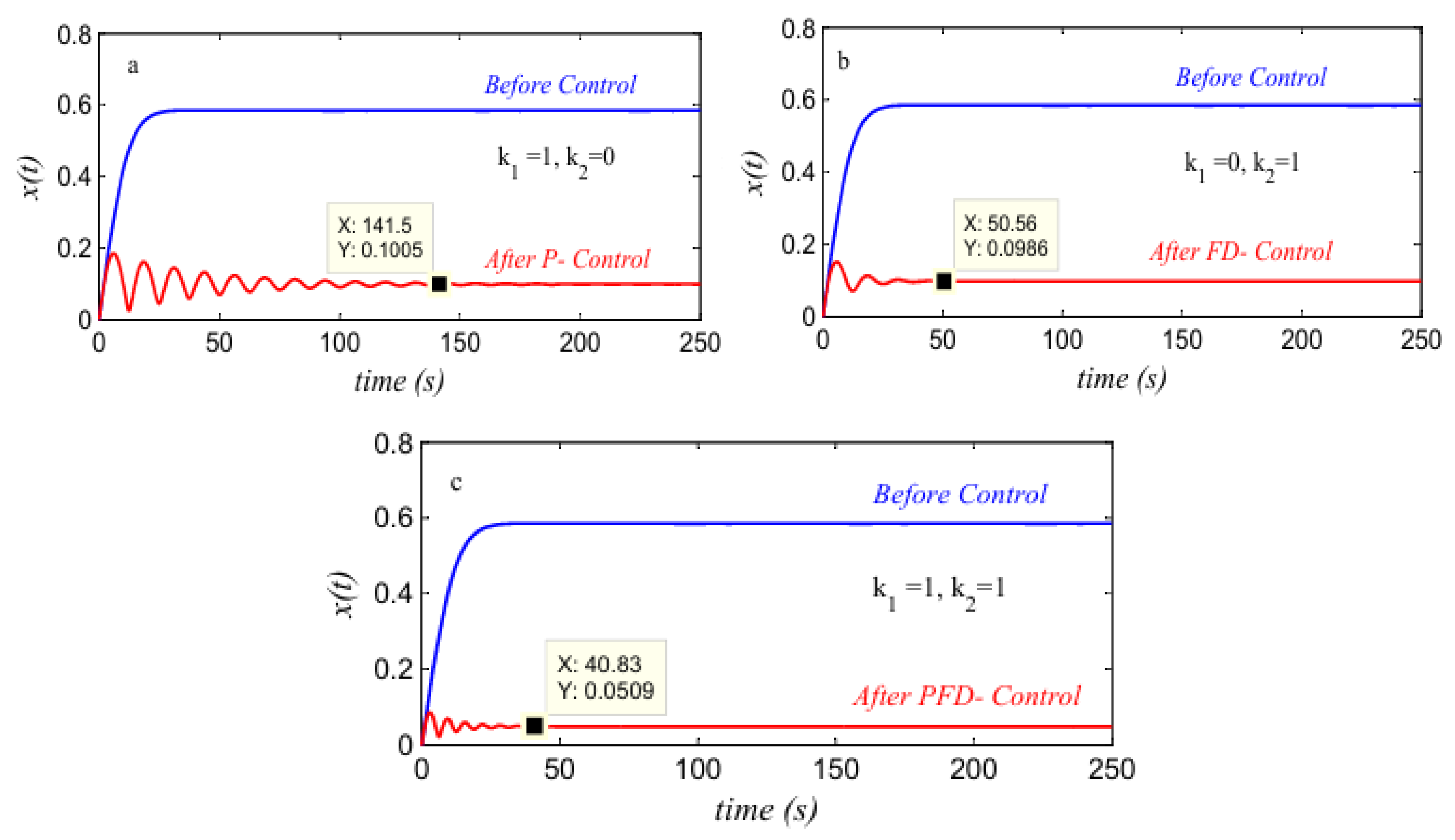
• The efficiency of the PD-Controller is equal to 8.
• The efficiency of the PFD-Controller is equal to 12.
• Adding the fractional derivative increases the efficiency of the PD-Controller in the primary resonance case ($\mathsf{\Omega }=\mathsf{\omega }$), i.e., at $\mathsf{\sigma }=0$.

References

1. Onur Ekici, H.; Boyaci, H. Effects of non-ideal boundary conditions on vibrations of microbeams. J. Vib. Control 2007, 13, 1369–1378. [Google Scholar] [CrossRef]
2. Kuang, J.H.; Chen, C.J. Dynamic characteristics of shaped micro-actuators solved using the differential quadrature method. J. Micromech. Microeng. 2004, 14, 647–655. [Google Scholar] [CrossRef]
3. Abdel-Rahman, E.M.; Younis, M.I.; Nayfeh, A.H. Characterization of the mechanical behavior of an electrically actuated microbeam. J. Micromech. Microeng. 2002, 12, 759–766. [Google Scholar] [CrossRef]
4. Younis, M.I.; Nayfeh, A.H. A study of the nonlinear response of a resonant microbeam to an electric actuation. Nonlinear Dyn. 2003, 31, 91–117. [Google Scholar] [CrossRef]
5. Amer, Y.A.; EL-Sayed, A.T.; EL-Salam, M.A. Non-linear Saturation Controller to Reduce the Vibrations of Vertical Conveyor Subjected to External Excitation. Asian Res. J. Math. 2018, 11, 1–26. [Google Scholar] [CrossRef]
6. Eftekhari, M.; Ziaei-Rad, S.; Mahzoon, M. Vibration suppression of a symmetrically cantilever composite beam using internal resonance under chordwise base excitation. Int. J. Non-Linear Mech. 2013, 48, 86–100. [Google Scholar] [CrossRef]
7. Amer, Y.A.; Abd EL-Salam, M.N.; EL-Sayed, M.A. Behavior of a Hybrid Rayleigh-Van der Pol-Duffing Oscillator with a PD Controller. J. Appl. Res. Technol. 2022, 20, 58–67. [Google Scholar]
8. Amer, Y.A.; Abdullah, R.E.; Khaled, O.M.; Mahdy AM, S.; El-Salam, M.N. Vibration Control of Smooth and Discontinuous Oscillator via Negative Derivative Feedback. J. Vib. Eng. Technol. 2024, 12, 2351–2363. [Google Scholar] [CrossRef]
9. Baleanu, D.; Diethelm, K.; Scalas, E.; Trujillo, J.J. Fractional Calculus: Models and Numerical Methods; World Scientific: Singapore, 2012; Volume 3. [Google Scholar]
10. Monje, C.A.; Chen, Y.; Vinagre, B.M.; Xue, D.; Feliu-Batlle, V. Fractional-Order Systems and Controls: Fundamentals and Applications; Springer: London, UK, 2010. [Google Scholar]
11. Mainardi, F. Fractional Calculus and Waves in Linear Viscoelasticity: An Introduction to Mathematical Models; World Scientific: Singapore, 2010. [Google Scholar]
12. El-Shourbagy, S.M.; Saeed, N.A.; Kamel, M.; Raslan, K.R.; Nasr, E.A.; Awrejcewicz, J. On the Performance of a Nonlinear Position-Velocity Controller to Stabilize Rotor-Active Magnetic-Bearings System. Symmetry 2021, 13, 2069. [Google Scholar] [CrossRef]
13. El-Shourbagy, S.M.; Saeed, N.A.; Kamel, M.; Raslan, K.R.; Aboudaif, M.K.; Awrejcewicz, J. Control Performance, Stability Conditions, and Bifurcation Analysis of the Twelve-Pole Active Magnetic Bearings System. Appl. Sci. 2021, 11, 10839. [Google Scholar] [CrossRef]
14. Saeed, N.A.; El-Shourbagy, S.M.; Kamel, M.; Raslan, K.R.; Aboudaif, M.K. Nonlinear dynamics and static biforcations control of the 12-pole magnetic bearings system utilizing the integral resonant control strategy. J. Low Freq. Noise Vib. Act. Control 2022, 13, 2069. [Google Scholar] [CrossRef]
15. Saeed, N.A.; El-Shourbagy, S.M.; Kamel, M.; Raslan, K.R.; Awrejcewicz, J.; Gepreel, K.A. Suppressing the resonant vibrations and eliminating the nonlinear bifurcation of a twelve-poles electro-magnetic rotor system using a novel control algorithm. Appl. Sci. 2022, 12, 8300. [Google Scholar] [CrossRef]
16. El-Salam, M.N.A.; Amer, Y.A.; Darwesh, F.O. Effect of negative velocity feedback control on the vibration of a nonlinear dynamical system. Int. J. Dyn. Control 2023, 11, 2842–2855. [Google Scholar] [CrossRef]
17. Ibrahim, K. Optimal PI–PD Controller Design for Pure Integrating Processes with Time Delay. J. Control Autom. Electr. Syst. 2021, 32, 563–572. [Google Scholar] [CrossRef]
18. Wang, Z.; Hu, H. Stability of a linear oscillator with damping force of the fractional-order derivative. Sci. China Phys. Mech. Astron. 2010, 53, 345–352. [Google Scholar] [CrossRef]
19. Wang, Z.H.; Du, M.L. Asymptotical behavior of the solution of a SDOF linear fractionally damped vibration system. Shock Vib. 2011, 18, 257–268. [Google Scholar] [CrossRef]
20. Leung AY, T.; Yang, H.X.; Zhu, P. Neimark bifurcations of a generalized Duffing–van der Pol oscillator with nonlinear fractional order damping. Int. J. Bifurc. Chaos 2013, 23, 1350177. [Google Scholar] [CrossRef]
21. Leung, A.Y.; Guo, Z. Forward residue harmonic balance for autonomous and non-autonomous systems with fractional derivative damping. Commun. Nonlinear Sci. Numer. Simul. 2011, 16, 2169–2183. [Google Scholar] [CrossRef]
22. Leung AY, T.; Yang, H.X.; Guo, Z.J. The residue harmonic balance for fractional order van der Pol like oscillators. J. Sound Vib. 2012, 331, 1115–1126. [Google Scholar] [CrossRef]
23. Xie, F.; Lin, X. Asymptotic solution of the van der Pol oscillator with small fractional damping. Phys. Scr. 2009, 2009, 1–4. [Google Scholar] [CrossRef]
24. Barbosa, R.S.; Machado, J.T.; Vinagre, B.M.; Calderon, A.J. Analysis of the Van der Pol oscillator containing derivatives of fractional order. J. Vib. Control 2007, 13, 1291–1301. [Google Scholar] [CrossRef]
25. Cui, Z. Primary resonance and feedback control of the fractional Duffing-van der Pol oscillator with quintic nonlinear-restoring force. AIMS Math. 2023, 8, 24929–24946. [Google Scholar] [CrossRef]
26. Podlubny, I. Fractional Differential Equations, Mathematics in Science and Engineering; Elsevier: Amsterdam, The Netherlands, 1999. [Google Scholar]
27. Nayfeh, A.H. Problems in perturbation. Appl. Opt. 1986, 25, 3145. [Google Scholar]
28. Han, R. A memory-free formulation for determining the non-stationary response of fractional nonlinear oscillators subjected to combined deterministic and stochastic excitations. Nonlinear Dyn. 2023, 111, 22363–22379. [Google Scholar] [CrossRef]
29. Wang, G.; Ma, L. A Dynamic Behavior Analysis of a Rolling Mill’s Main Drive System with Fractional Derivative and Stochastic Disturbance. Symmetry 2023, 15, 1509. [Google Scholar] [CrossRef]
30. Zhang, Y.; Han, R.; Zhang, P. Stochastic response of chain-like hysteretic MDOF systems endowed with fractional derivative elements and subjected to combined stochastic and periodic excitation. Acta Mech. 2024, 235, 5019–5039. [Google Scholar] [CrossRef]
Figure 1. Cantilever beam structure.
Mathematics 13 01886 g001
Figure 2. Closed-loop control system.
Mathematics 13 01886 g002
Figure 3. (a) Response of the cantilever beam to time t without control ( k 1 = k 2 = 0 ) at three different levels of the external force; (b) σ –response curves corresponding to (a) f = 0.05 , 0.1, and f = 0.2 .
Mathematics 13 01886 g003
Figure 4. (a) Response of the cantilever beam to time t when the P-Controller is ON ( k 1 = 2.5 ) and the FD-Controller is OFF ( k 2 = 0 ) at three different levels of the external force; (b) σ –response curves corresponding to (a) f = 0.05 , 0.1, and f = 0.2 .
Mathematics 13 01886 g004
Figure 5. (a) Response of the cantilever beam to time t when the P-Controller is OFF ( k 1 = 0 ) and the FD-Controller is ON ( k 2 = 2.5 ) at three different levels of the external force; (b) σ –response curves corresponding to (a) f = 0.05 , 0.1, and f = 0.2 .
Mathematics 13 01886 g005
Figure 6. (a) Response of the cantilever beam to time t when the PFD-Controller is ON ( k 1 = k 2 = 2.5 ) at three different levels of the external force; (b) σ –response curves corresponding to (a) f = 0.05 , 0.1, and f = 0.2 .
Mathematics 13 01886 g006
Figure 7. (a) Response of the cantilever beam to time t when the PFD-Controller is ON at three different levels of the fractional-order derivative; (b) α –response curves at f = 0.1 .
Mathematics 13 01886 g007
Figure 8. Response of the cantilever beam’s peak to time t when (a) the P-Controller is ON and the FD-Controller is OFF, (b) the P-Controller is OFF and the FD-Controller is ON, and (c) the PFD-Controller is ON at f = 0.1 and α = 0.5 .
Mathematics 13 01886 g008
Figure 9. Comparison between the PD-Controller ( α = 1 ) and the PFD-Controller ( α = 0.1 ).
Mathematics 13 01886 g009