1. Introduction
Let G be a simple undirected graph of order n with vertex set and edge set . The cardinality of a set S is denoted by . For let and denote the set of neighbors of vertex u and , respectively. The degree of the vertex u is .
The multiset of the eigenvalues of a symmetric square matrix M is called the spectrum of M and is denoted by .
If
is an
complex matrix and
is an
non-negative matrix such that
(
for all
), then
M is said to dominate
C. For more properties of matrix, see [
1,
2].
The distance between the vertices
and
in a connected graph
G is denoted by
, and the diameter of
G is defined as
The maximum degree matrix
of
G, as defined in [
3], is the square matrix of order
n whose
-entry is equal to
if the vertices
and
are adjacent, and 0 otherwise.
Let
be the characteristic polynomial of
, that is,
In [
3], Adiga et al. established the coefficients
of
for
in
.
The eigenvalues of are called the maximum degree eigenvalues of G. To develop our results, we denote the spectral radius of by .
We use the summation symbol to add numbers, as is commonly done, and also to sum or subtract edges in a graph.
In a graph
G without isolated vertices, the maximum degree matrix
is a non-negative irreducible matrix. By the Perron–Frobenius Theorem, there exists an eigenvector of
associated with the spectral radius
with strictly positive entries. We denote this eigenvector as
or simply
, and it is called the principal eigenvector of
. Any other eigenvector associated with
is a scalar multiple of
. For more properties of graphs, see [
4,
5]
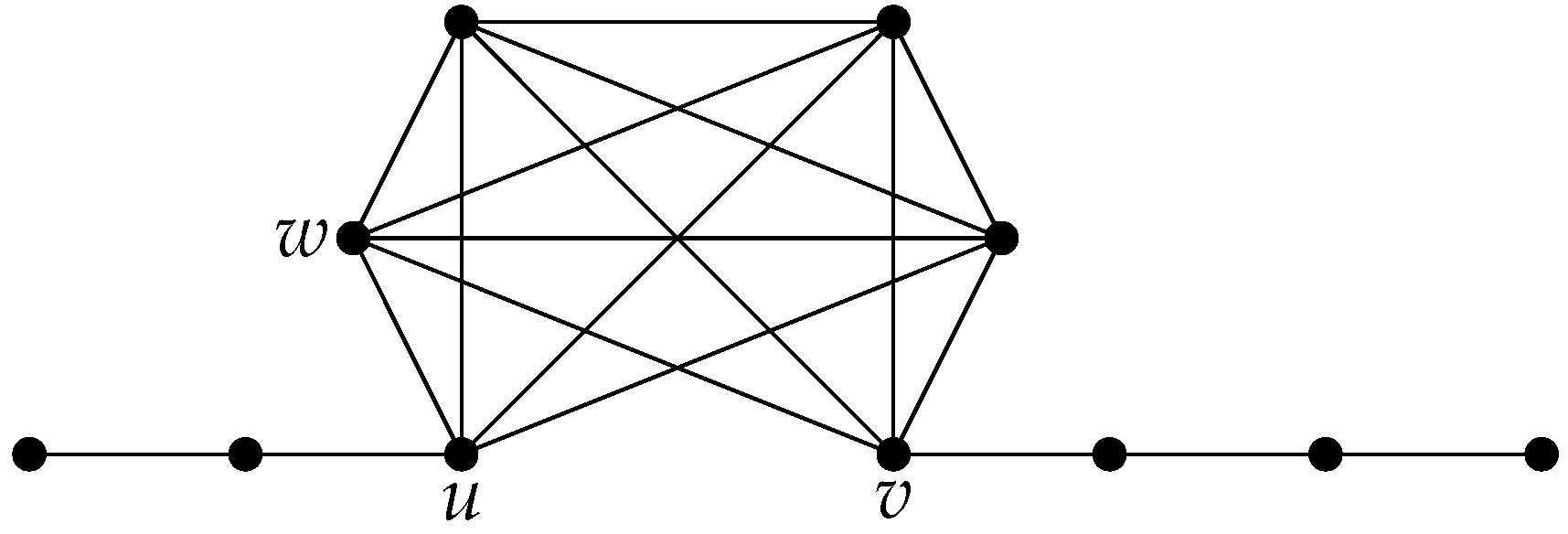
Let
be the graph obtained from a complete graph
by deleting an edge
and identifying the vertices
u and
v with the end vertices
and
of the paths
and
, respectively; see
Figure 1. Observe that
is a graph on
vertices and
.
In [
6], the authors show that the graph
maximizes the spectral radius among graphs with
n vertices and diameter
. In [
7], the authors prove that for the given positive integers
n and
, among all connected graphs of order
n and diameter
d, the maximal signless Laplacian spectral radius is attained uniquely by the graph
. In [
8], several extremal results are presented concerning the spectral radius of the matrix
, where
, which generalizes the two previous results. Here,
A and
D denote the adjacency and degree diagonal matrices of the graph, respectively.
The goal of this paper is to show that among all graphs of order n and diameter , the graph that uniquely attains the largest spectral radius of the maximum degree matrix is . Furthermore, we characterize the maximum degree eigenvalues of for . Finally, if is an even integer, the spectral radius of the maximum degree matrix of can be computed as the largest eigenvalue of a symmetric tridiagonal matrix of order .
3. Results
In this section, we begin by recalling the following definition.
Definition 1 ([
11]).
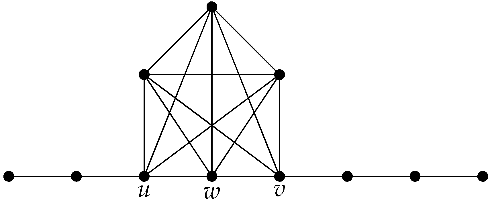
Let G be a connected graph. A path P in G with end vertices u and v is called a diametral path of G if P has vertices and . Let
with
. For
, the graph
with
n vertices is isomorphic to the graph obtained from the complete graph
and a path
P with
vertices,
, by adding edges to connect each vertex of the complete graph
with the vertices
(
Figure 2).
For each connected graph
G, we label the vertices of
G such that the first
vertices,
are the vertices of a diametral path in
G. Let
Lemma 4. Let G be a connected graph. Let . If , then Proof. Let with (if , we proceed analogously). We claim that . Suppose . Then, there are at least two vertices with .
Thus, the set of vertices
can be used to build a new path of length less than
connecting
to
, which is a contradiction. Therefore, the result follows. □
In the following result, we denote the complement of by Note that if and only if .
Lemma 5. Let G be a connected graph on the vertices n. Let . Then, there exists a graph with n vertices and a diameter less than or equal to such that G is a subgraph of which verifies the following conditions:
- 1.
The vertices in are the vertices of the complete graph; - 2.
Each vertex in is adjacent to exactly three consecutive vertices in ;
- 3.
Proof. Let G be a connected graph on n vertices. Clearly, we can see that in the process of adding edges between the vertices in the diameter of the new graph is less than or equal to . We construct the graph as follows:
- 1.
Starting with G, we construct a graph by adding edges, if necessary between the vertices in , until these form the complete graph .
- 2.
As per Lemma 4, each vertex in is adjacent to at most three consecutive vertices . Finally, we construct the graph , adding edges in such that each vertex in is adjacent exactly to three consecutive vertices in .
- 3.
It follows from Lemma 2.
The proof is complete. □
Remark 1. Note that if G is a path on n vertices, then Let be a connected graph as in Lemma 5. Note that the vertices of in are the vertices of the complete graph . Considering , we will say that the two vertices u and v in are related if and only if . Note that the above is an equivalence relation. Let be the cliques in determined by the equivalence classes of the above relation.
The cliques have the following properties:
- 1.
All the vertices in are connected to the same three consecutive vertices in , for .
- 2.
Each vertex in is adjacent to all the vertices in for .
Considering the construction of starting from the graph G, we can assume, without a loss of generality, the following:
If ,
and
then
.
Thereby, by the construction of the graph , the following result is an immediate consequence of Lemma 5.
Theorem 1. Let with . Let be as in Lemma 5 with . Then,for some . Corollary 2. Let and . Then, Lemma 6 ([
12]).
Let N be a non-negative irreducible symmetric matrix with the spectral radius . If there exists a positive vector and a positive real β such that , then . Definition 2 ([
13]).
An internal path in a graph G is a path with a sequence of distinct vertices , , where is adjacent to , , , , and for all . Remark 2. If the number of cliques , we reduce to a having the spectral radius of the maximum degree matrix larger than . This would be achieved by induction on s. In this process, the following result plays an important role in this work.
Lemma 7. Let G be a connected graph with n vertices and some edge on an internal path with vertices of respectively. We subdivide the edge by a vertex such that the edges , are added to G. We denote this new graph as . Then, Proof. Let be the principal eigenvector of and be the corresponding component of . Clearly, . By replacing the labels if necessary we may assume that .
So, Without a loss of generality, we may assume that , .
If , take to be the vector obtained from by inserting an additional component equal to between the positions t and .
For the vertex
u, we have
For the vertex
w, we have
Then, . By Lemma 6, we have .
Consequently, we will suppose that . Let S be the set of neighbors of other than , and let .
If , then we construct as above with .
For the vertex
u, we have
For the vertex
w, we have
If
, then
, so the strict inequality in (
3) is true. Then,
. By Lemma 6, we have
.
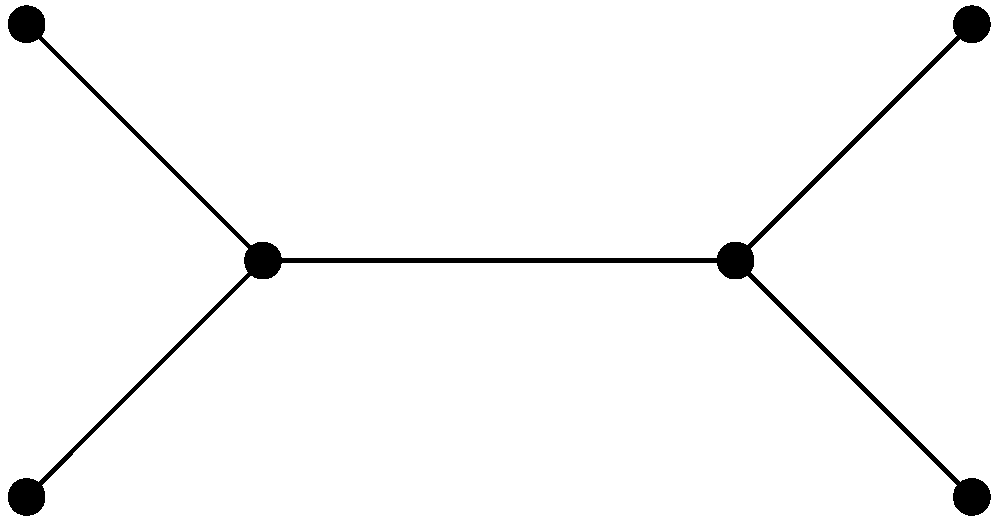
Let
, and suppose the equalities (
2) and (
3) are true. Then,
and
. Since
and the graph
depicted in
Figure 3 is a proper subgraph of
G, then
where
is the spectral radius of
, which is a contradiction. Then,
. By Lemma 6, we have
.
Finally, suppose that . In this case, we construct from by replacing with s and inserting equal to .
For the vertex
w, we have
Therefore, it follows that
. By Lemma 6, we have
The proof is complete. □
Definition 3 ([
14]).
The contraction of an edge in a graph G is the identification of the vertices u and v into a single vertex w such that the edges incident to w are precisely the distinct edges (excluding ) that were incident to either u or v in G. Theorem 2. Let with . Let be as in Lemma 5 and let . Then,for some . Proof. Let G be a connected graph with n vertices and . Let be as in Lemma 5 and . Considering the construction of graph , we can assume without a loss of generality that
and
for some
. Keeping the previous notation in mind, four situations can occur in the graph
:
,
,
, and
(
Figure 4).
Case:
Let
and
where
and
.
Clearly,
and
. By application of Corollary 1, we obtain
where
or
.
Since in , all vertices in are adjacent to the same three consecutive vertices in , by Theorem 1, we obtain the result.
For Case , we have .
Let
and
be as in (
4) and (
5), respectively, where
and
. Clearly,
and
.
By application from Corollary 1, we get
where
or
.
Suppose . If , by Lemma 7, we have where is the graph obtained of by the contraction of the edge to a new vertex . Let be the graph obtained of by attaching a new pendant vertex to the vertex . By Lemma 2, .
Suppose . Let be the graph obtained of by attaching a new pendant vertex to the vertex . By Lemma 2, . By Lemma 7, we get where is the graph obtained of by the contraction of the edge to a new vertex . The cliques and in are as in . By applying to , the result follows.
If , then the way to reason is analogously.
Case:
Let
and
be as in (
4) and (
5), respectively, where
and
. Clearly,
and
. By application of Corollary 1, we get
where
or
.
Suppose . By Lemma 7, we have , where is the graph obtained of by the contraction of the edge to a new vertex . By Lemma 2, we obtain , where is the graph obtained of by attaching a new vertex to one of the pending vertices. The cliques and in are as in . By applying to , the result follows.
If , then the way to reason is analogously.
Case: with .
By Lemma 7, we have , where is the graph obtained of after contracting edges on the internal path . By Lemma 2, we get , where is the graph obtained of by attaching a path on vertices to one of the pending vertices. The cliques and in are as in . By applying to , the result follows. □
As an immediate consequence of Theorems 1 and 2, we obtain the following result.
Corollary 3. Let and . Then, Theorem 3. Let . Let be as in Lemma 5. Let . Then,for some . Proof. Applying induction on s. The case is given in Theorem 2. Let . Suppose that the result holds for .
First, suppose that there exist two cliques and satisfying condition (A) in Theorem 2. In this case, and are reduced to a single clique such that their vertices are connected to the same three consecutive vertices in . By the induction hypothesis, the result follows.
Now, suppose that there is no pair of cliques satisfying condition (A) as in Theorem 2. Then, we consider the two cliques and and apply the techniques used in cases (B), (C), or (D) of Theorem 2 to reduce them to a single clique whose vertices are connected to the same three consecutive vertices in . Again, by the induction hypothesis, the result follows. □
4. The Largest Spectral Radius of the Maximum Degree Matrix Among All Graphs with a Given Order and Diameter
In this section, we characterize the maximum degree eigenvalues of for . In particular, we prove that is always an eigenvalue of with multiplicity , and that the remaining eigenvalues are precisely the eigenvalues of a non-negative symmetric tridiagonal matrix of order .
4.1. Maximum Degree Eigenvalues of with
We recall that given two disjoint graphs
and
, the join of
and
is the graph
, such that
and
This operation can be generalized as follows [
14,
15]. Let
H be a graph with
k vertices, and let
. Let
be a family of pairwise disjoint graphs. For each
j, the vertex
is assigned to the graph
. Let
G be the graph obtained from the graphs
and the edges connecting every vertex of
to all vertices of
for each edge
. That is,
This graph is called the
H-join of the graphs
and is denoted by
If
is the order of
for
, then the
H-join of
is a graph of order
.
Examples of this operation on graphs can be seen in the graphs . In fact, is the -join of the regular graphs , , . For , and the graph is the -join of the graphs , , .
Example 1. The graph as a -join is the graph in Figure 5: In [
14], the spectrum of the adjacency matrix of the
H-join of regular graphs is obtained. The version of this result for the maximum degree matrix is given below, and its proof is analogous.
Theorem 4. If and is a graph -regular for , thenwhere is the i-th eigenvalue of the adjacency matrix of andfor . Remark 3. Now, we denote by I the identity matrix, J the matrix with ones on the skew diagonal, and F the matrix whose entries are all zeros except for the entry in the last row and first column, which is equal to . The order of each of these matrices is clear from the context in which they are used.
Definition 4 Let and The application of Theorem 4 to each graph
allows us to characterize its maximum degree eigenvalues. We begin by introducing the matrix
, and for
, the symmetric tridiagonal matrix of order
Clearly,
. From the recursion formula for symmetric tridiagonal matrices [
16], we have
where
,
and
.
Theorem 5. Let . The maximum degree eigenvalues of
are with multiplicity and the eigenvalues of the symmetric tridiagonal matrix of order whereandwhen . Corollary 4. The largest eigenvalue of is the spectral radius of the maximum degree matrix of . The eigenvalues of are simple.
Proof. From Theorem 5, the maximum degree eigenvalues of are and the eigenvalues of . Let be the largest eigenvalue of . Since the largest eigenvalue of a Hermitian matrix is greater than or equal to any diagonal entry, it follows that . Then is the spectral radius of the maximum degree matrix of . Since is a symmetric tridiagonal matrix with nonzero co-diagonal entries, its eigenvalues are simple. □
4.2. Determination of the Maximizing Graph in
In this subsection, we determine the graph with the largest spectral radius of the maximum degree matrix among all connected graphs with a given diameter.
Lemma 8. Let and . Let T be the symmetric tridiagonal matrix of order given bywhereandThenand particularly, . Proof. Considering that
, we have
Then,
. Note that
is a matrix whose entries are zero except the entry in the last row and the last column which is equal to
. Finally, by Lemma 3, the result follows. □
Lemma 9. Let and . Then, Proof. Applying a similar argument as in Lemma 8 to
with
and
, we have
Suppose that
. Analogously, if
and
, we have
For
, Equation (
8) is immediate by (
6) and
. Considering (
7) and (
8), the result follows. □
By repeatedly applying Lemma 9, we obtain the following result.
Remark 4. We will now discuss the difference between the characteristic polynomials of and . From Lemma 8,where with . Replacing this in (9) and using and , we haveLet . By Lemma 8,where , , with . By applying Lemma 8 to and , we haveandBy replacing these identities in (10), we haveConsequently, for , we haveBy applying Corollary 5 on the four polynomial differences of the last identity, we haveFrom the recursion formula for symmetric tridiagonal matrices [16], we haveConsidering thatThrough simple algebraic calculations, we havewhereTherefore, Since and are isomorphic graphs, for , we prove the following result.
Theorem 6. Let with . Then,for Proof. Let
. We know, by Corollary 4, that the spectral radius of the maximum degree matrix of
is the largest eigenvalue of the matrix
of the order
. Let
and
the eigenvalues of the matrices
and
, respectively. Then
and
By (
11), we have
Thereby,
Considering
, we get
We claim that
. Suppose that
. Then,
for
. Then, the left side of (
12) is non-negative. Clearly,
which implies
. Furthermore,
and
, then the right side of (
12) is negative, which is a contradiction. Therefore,
. □
Theorem 7. Let with . Then,the equality is given if and only if . Proof. If the result is verified by Corollaries 2 and 3. Now, let . Suppose . The result is verified by Theorems 1, 3 and 6. Now, suppose . By Remark 1, . The proof is complete. □
Theorem 8. Let . Then, Proof. Let
be the vertices in a diameter path of
We obtain a new graph
, and add two edges that connect the vertex
with the two vertices
. By Lemma 2,
It is easy to see that
has diameter
d. If
, by Theorem 6, we have
, the result is verified. Suppose
. Let
. We obtain a graph
and add edges that connect the vertex
with all the vertices of
.
Considering the construction of graph
, we have
and
for each
. Keeping the previous notation in mind, four situations can occur in the graph
as mentioned below:
- (A)
- (B)
- (C)
- (D)
.
Using the same techniques in the proof of Theorem 2, cases (A), (B), (C) and (D), with
and
, we can conclude that
for some
.
From (
13), (
14), (
15) and Theorem 6, the proof is complete. □
Theorem 9. Let G be a connected graph on n vertices and let . If , then . If , thenThe equality holds if and only if . Proof. If , then . Let . Let be the graph with the largest spectral radius of the maximum degree matrix among all the graphs on n vertices and diameter greater than or equal to d. Suppose .
By Theorem 7,
Let
. By Theorem 8, we have
which is a contradiction. Then,
. Due to Theorem 7, the proof is complete. □
5. Computing the Largest Spectral Radius of the Maximum Degree Matrix of Graphs with a Given Order and Diameter
Among various graph matrices, the maximum degree matrix has emerged as a recent tool to capture interactions between vertex degrees and adjacency. Given a graph G, this matrix encodes, for each edge, the maximum degree between the incident vertices, and zero otherwise.
In this context, an important extremal problem arises: identifying connected graphs, among all those with a fixed number of vertices n and diameter that maximize the spectral radius of their maximum degree matrix. This problem not only deepens our understanding of the spectral behavior of such matrices but also connects with classical extremal graph theory and structural optimization.
This section focuses on the analytical computation of the largest possible spectral radius of the maximum degree matrix among all graphs with fixed order and diameter, using known characterizations and structural properties of special graph classes.
From Theorem 5, can be computed as the largest eigenvalue of the symmetric tridiagonal matrix .
Theorem 10. If , then can be computed as the largest eigenvalue of the symmetric tridiagonal matrix of order 4 with diagonal entriesand co-diagonal entriesIf , then can be computed as the largest eigenvalue of the symmetric tridiagonal matrix with diagonal entriesand co-diagonal entries In [
17], the authors show that the signless Laplacian spectral radius of
can be computed as the largest eigenvalue of a symmetric tridiagonal matrix of the order
whenever
d is an even integer. The corresponding version of this result for the maximum degree matrix is given below.
Theorem 11. If is an even integer, then can be computed as the largest eigenvalue of a symmetric tridiagonal matrix of the order with the diagonaland co-diagonal entries Proof. Let
d be an even integer. From Theorem 10,
can be computed as the largest eigenvalue of
of order
, where
.
Consider the orthogonal matrix
Simple algebraic calculations show that
Then, the eigenvalues of
are the eigenvalues of
and the eigenvalues of
U. Since that the eigenvalues of
U strictly interlace the eigenvalues of
. □


