Distributed Observer-Based Adaptive Trajectory Tracking and Formation Control for the Swarm of Nonholonomic Mobile Robots with Unknown Wheel Slippage

Abstract

Nonholonomoic mobile robots (NMRs) are widely used in logistics transportation and industrial production, with motion control remaining a key focus in current WMR research. However, most previously developed controllers assume ideal conditions without considering motion slippage. Neglecting slippage factors often leads to reduced control performance, causing instability and deviation from the robot’s path. To address such a challenge, this paper proposes an intelligent method for estimating the longitudinal wheel slip, enabling effective compensation for the adverse effects of slippage. The proposed algorithm relies on the development of an adaptive trajectory tracking controller for the leader robot. This controller enables the leader robot to accurately follow a virtual reference trajectory while estimating the actual slipping ratio with precision. By employing this approach, the mobile robot can effectively address the challenge of wheel slipping and enhance its overall performance. Next, a distributed observer is developed for each NMR that uses both its own and adjacent robot’s information to determine the leader’s state. To solve this difficulty for the follower robot to receive the states of the leader in a large group of robots, distributed formation controllers are designed. Further, Lyapunov stability theory is utilized to analyze the convergence of tracking errors that guarantees multi-robot formation. At last, numerical simulations on a group of NMR are provided to illustrate the performance of the designed controller. The leader robot achieved a low RMSE of 1.7571, indicating accurate trajectory tracking. Follower robots showed RMSEs of 2.7405 (Robot 2), 3.0789 (Robot 4), and 4.3065 (Robot 3), reflecting minor variations due to the distributed control strategy and local disturbances.

1. Introduction

Mobile robots have gained extensive utilization across diverse domains, owing to the remarkable progress in robot technology [1]. The utilization of multiple mobile robots working in cooperation offers various applications, including target search, visual servoing, path planning, human motion tracking, and intelligent video surveillance and transportation. Compared to single mobile robots, a system comprising multiple mobile robots provides additional benefits such as fault tolerance, flexibility, and improved task efficiency. Among the various applications of wheeled mobile robot systems, formation control stands out as a fundamental and critical research topic. In general, the purpose of formation control in robots is to ensure that each robot achieves the necessary velocity to maintain the prescribed formation pattern of the entire robot system.

Extensive research has been conducted on the topic of formation control for multiple mobile robots. Commonly employed control techniques include virtual structure methods, behavior-based approaches, and leader-following-based approaches. Among these, leader-following approaches have gained increasing attention due to their favorable properties, such as ease of implementation, analysis, and flexibility. However, it is worth noting that previous works assume that all followers acquire precise information about the leader’s state, which can often be challenging and complex to obtain in real-world scenarios. Factors like communication bandwidth, the operating distance between robots, and the total number of robots in the system can affect the followers’ ability to acquire precise information about the leader. Hence, it seems more reasonable to assume that merely a fraction of the team’s mobile robots had direct access to the leader’s status. In order to learn more about the leaders, it is crucial to investigate distributed estimating methodologies for each robot.

Likewise, the method presented in [2], which uses broadcast control with norm-limited update vectors for multi-robot systems, achieves coordinated behavior while ensuring system stability by limiting the update magnitudes. Although it simplifies communication and control in large-scale robotic networks, it still faces challenges concerning communication reliability, scalability, and response time. Another work [3] addresses the formation control problem for second-order multi-agent systems with actuator saturation and input coupling. An estimator-based robust formation controller is developed to guarantee the boundedness of the formation tracking error. Furthermore, to estimate system uncertainties without requiring prior knowledge of their Lipschitz constants, two novel estimators are proposed by integrating neural-based estimation with the sliding mode technique.

To analyze the stability properties of leader–follower relationships, nonlinear gain estimates in the formation structure are studied and applied to mobile robot formations in [4]. In [5], the leader–follower scheme was developed for swarm formation of NMRs with respect to velocity control and generating smooth trajectories for the follower. A receding-horizon control framework for leader–follower control was proposed in [6]. On the other hand, an adaptive PID algorithm has been utilized for formation control in [7]. Also, the leader–follower formation strategy has been presented for multiple NMRs without considering the position and velocity measurements in [8]. As is evident, the leader–follower formation of multiple NMRs to address the velocity tracking problem has been presented in [9]. This study proposes a novel switched-system approach, combining bang-bang control and consensus algorithms, to achieve time-optimal velocity tracking for multiple nonholonomic wheeled mobile robots under arbitrary initial conditions. To overcome the effects of kinematic disturbances, an observer-based PID controller is presented for NMR and implemented in a real platform [10]. An adaptive terminal integral SMC method has been created to address challenges posed by unanticipated bounded disturbances and uncertainties in NMR trajectory problems [11]. Although it is assumed in the existing literature that each follower can access information about the leader robots, this is difficult to achieve in practice when the number of robots expands.

Various distributed control methodologies have emerged, leveraging graph theory, to cater to the needs of nonholonomic mobile robots operating within diverse network structures. These methodologies have specifically tackled formation problems at both the robot kinematic and dynamic levels. The authors of [12] tackles the tracking control problem for a group of nonholonomic wheeled mobile robots with partial information about the desired trajectory. By utilizing communication between the systems, distributed control laws are proposed to ensure that the state of each mobile robot asymptotically tracks the desired trajectory. The task of tracking trajectories for a wheeled mobile robot while contending with kinematic and dynamic uncertainties as well as disturbances linked to the sliding velocity has been tackled [13]. A new controller is proposed for visual servoing trajectory tracking of nonholonomic mobile robots without requiring direct position measurement [14]. To eliminate the need for global position sensing, a novel adaptive estimator is developed to estimate the robot’s global position online, using natural visual features captured by a vision system along with orientation and velocity data from odometry and AHRS sensors. In [15], the formation tracking controller has been developed for mobile robot systems using a distributed controller, which is intended to meet the velocity limitations. In [16] a single time-varying controller was developed using the Lyapunov method to simultaneously address the asymptotic regulation and tracking problems of a mobile robot. Using the distributed nonlinear controllers, authors in [17] have analyzed the formation control of unicycle robots without considering general posture dimensions. Subsequently, a finite-time control is presented in [18], where the distributed observer is developed for the multiple NMRs.

The formation control problem for several NMR is transformed into a consensus problem in [19]. In [20], the authors changed the nonholonomic systems to a chained form and then the challenge is solved by using a dynamic oscillator. In [21], a robust tracking control method was developed for multiple uncertain NMRs with limited communication ranges. A model predictive approach is exploited in the distributed controller to maintain the desired formation towards the desired trajectory which assures no collisions with obstacles in [22]. To improve the tracking efficacy, a distributed estimation-based control method is designed for the follower NMRs in [23]. In [24], a distributed estimator is employed to asymptotically generate the leader NMR’s state estimates at each follower, while a local tracking controller ensures each NMR follows the leader, achieving coordinated control. On the other hand, [25,26] investigates the formation control problem for multiple nonholonomic wheeled mobile robots using distributed estimators and a biologically inspired approach. Conversely, an adaptive estimator and an adjusted gradient control law have been formulated using nonholonomic kinematics principles, aiming to guarantee the attainment of the desired formation shape within the system [27]. Moreover, the authors in [28] have investigated a distributed optimization method for the achievement of a desired collective behavior among the robots. The research on distributed control of NMRs has made valuable contributions. Recently, a distributed PI-DDILC algorithm was developed for NMR formation to reduce the complexity of the model and improve its efficiency [29]. Under the directed graph, distributed consensus control for NMR has been implemented by utilizing the leader position details [30]. However, the controllers proposed in these studies cannot be directly utilized in environments with slippage constraints, necessitating further research and modifications.

In the real world, wheeled mobile robots often experience slippage due to the presence of ice, sand, or muddy roads. This is because the reaction force from the ground is not always sufficient to overcome the driving strength of NMR. When the propulsive force surpasses the reactive force, wheel slippage can occur, potentially resulting in imprecise control and diminished performance. To date, few studies have considered the impact of slippage on the formation control of multi-robot systems. This is a significant oversight, as slippage can significantly complicate the design of controllers and can lead to the formation breaking apart. Future research should focus on developing formation control algorithms that are robust to slippage. This could be done by incorporating models of slippage into the controller design or by using adaptive control techniques. In [31], the study delved into the kinematics and dynamics model of several mobile robots experiencing skidding and slipping. The researchers developed an adaptive formation tracking controller that incorporates the capability to address unforeseen sliding and slippage effects, employing the dynamic surface design method. In [32], the distributed control was presented under directed networks which can perform the formation of NMRs in the presence of unknown skidding and slipping phenomena. In order to address the formation control challenge involving multiple mobile robots, the approach of incorporating the prescribed performance-bound method has been adopted, ensuring the prevention of collisions between any pair of robots [33]. Recently, the authors in [34] have presented the formation control approach using estimated information of the leader for multiple wheeled NMRs with longitudinal slippage constraints. Following this, the distributed observer was developed in [35] without considering the position details. However, it is important to note that these investigations were conducted within a centralized framework, where all follower robots had access to the leader robot’s information. As a result, tackling distributed formation control for multi-robot systems within the constraints of slippage presents a noteworthy challenge.

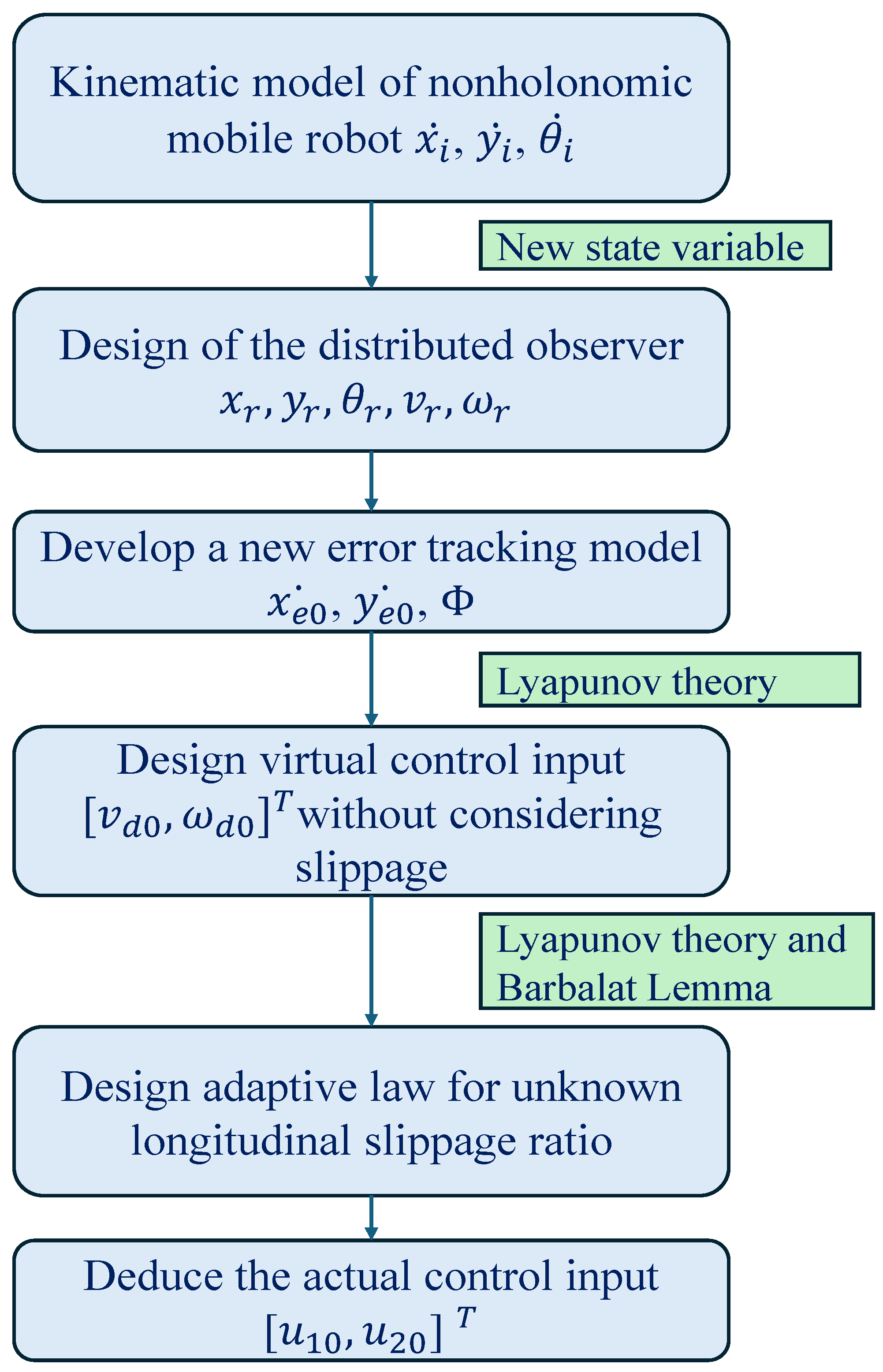
In this paper, we put forth an innovative and advanced distributed control method for a leader–follower multi-robot formation system, specifically addressing the challenging unknown slippage constraint. Our approach leverages cutting-edge techniques and introduces key contributions that significantly enhance the field of robot formation control. To begin, we introduce the concept of a “slipping ratio”, which serves as a robust model to accurately represent longitudinal sliding disturbances. This novel representation enables us to design new state variables that effectively capture the dynamics of the system. Building upon this foundation, we propose a trajectory tracking controller specifically tailored for the leader robot, along with an adaptive law for the slipping ratio. These innovations ensure precise control even in the presence of slipping, pushing the boundaries of what can be achieved in formation control.

Additionally, we tackle the challenge posed by the limited communication abilities of the individual robots within the system. To overcome this limitation, we employ distributed state observers, which enable each follower NMR to estimate the state information of the leader NMR by leveraging information from its neighboring robots and its own sensory inputs. This distributed estimation scheme paves the way for the design of formation controllers that utilize the estimated information. By leveraging this knowledge, our controllers facilitate the realization of the desired formation goal while effectively compensating for the adverse effects of slipping. Compared to existing works, the contributions of our research are manifold and substantial. We provide a comprehensive and integrated solution that addresses both the challenges of unknown slippage and limited communication. By leveraging innovative concepts and advanced control techniques, we push the boundaries of what can be achieved in robot formation systems, opening up new avenues for future research and practical applications.

The contributions of the paper are

1.

The tracking control problem of a single leader NMR with a reference trajectory is considered. Following that, a trajectory tracking controller is designed for the leader NMR to follow the predefined path of the reference trajectory. Different from the controllers used in [12,16], the proposed method uses adaptive trajectory tracking controllers and estimates the real value of the slipping ratio precisely.

2.

The distributed observer is incorporated for the follower NMR to suppress the needs of location measurements ensuring the prescribed leader–follower formation. Compared with earlier works [23,25], the key feature of the designed observer is the estimation of the leader’s linear and angular velocity. For this innovation, the formation pattern can be achieved without slippage effects using designed control laws.

3.

The aforementioned results [32,34] requires the position, orientation, and velocity information of the leader or neighboring NMR which increases the communication load. To overcome this problem, a distributed formation control law is developed to achieve the desired formation by employing the estimated state of the leader simultaneously combating the effects of slippage. Moreover, applying Lyapunov stability theory and cascaded system theory suggests some sufficient conditions are obtained to prove the system’s stability.

2. Problem Statement

2.1. Algebraic Graph Theory

The relationships between agents can be effectively represented as a graph. Let the network topology consists of $N+1$ robots. Consider, the followers (${\mathbb{V}}_N$) indexed by $1,2,\dots ,N$ and one leader (${\mathbb{V}}_0$) indexed by 0 in the group of NMRs. An undirected graph $\mathbb{G}=\mathbb{V},\mathbb{E},\mathbb{A}$ is described with $\mathbb{V}={\mathbb{V}}_1,{\mathbb{V}}_2,\dots ,{\mathbb{V}}_N$ be a node-set which represents N follower NMRs and the corresponding edge set $\mathbb{E}\subseteq \mathbb{V}\times \mathbb{V}$. In the undirected graph $\mathbb{G}$, an edge represented by $({\mathbb{V}}_j,{\mathbb{V}}_i)\in \mathbb{E}$ if and only if there exists a connection from ${\mathbb{V}}_i$ to ${\mathbb{V}}_j$. For the leader–follower formation, consider a group of NMR. A typical model of an NMR system is depicted in Figure 1.

The structure of the proposed leader–follower method is illustrated in Figure 2.

The design flowchart of adaptive controller of proposed leader–follower framework for NMRs is shown as Figure 3.

The adjacency matrix $\mathbb{A}=\left[a_{ij}\right]\in {\mathbb{R}}^{N\times N}$ of $\mathbb{G}$ is defined as

$$\begin{array}{c}\hfill a_{ij}=\left\{\begin{array}{c}\begin{array}{cc}1,& \mathrm{for} ({\mathbb{V}}_j,{\mathbb{V}}_i)\in \mathbb{E},\\ 0,& \mathrm{otherwise}.\end{array}\hfill \end{array}\right.\end{array}$$

(1)

Throughout this paper, we make the assumption that $a_{ii}=0$ for all ${\mathbb{V}}_i$. The Laplacian matrix of $\mathbb{A}$ is given by

$$\begin{array}{c}\hfill l_{ij}=\left\{\begin{array}{c}\begin{array}{cc}-a_{ij},& {\mathbb{V}}_i\ne {\mathbb{V}}_j,\\ \sum _{j=1,j\ne i}^n{a}_{ij},& {\mathbb{V}}_i={\mathbb{V}}_j.\end{array}\hfill \end{array}\right.\end{array}$$

(2)

The leader adjacency matrix is denoted as

$$\begin{array}{c}\hfill a={[a_{10},a_{20},\dots ,a_{n0}]}^T,\end{array}$$

(3)

where, the adjacency weight $a_{i0}$ defined as

$$\begin{array}{c}\hfill a_{i0}=\left\{\begin{array}{c}\begin{array}{cc}1,& \mathrm{if}{\mathbb{V}}_0\mathrm{is}\mathrm{a}\mathrm{neighbor}\mathrm{of}{\mathbb{V}}_i,\\ 0,& \mathrm{otherwise}.\end{array}\hfill \end{array}\right.\end{array}$$

(4)

The matrix $\mathbb{H}\in {\mathbb{R}}^{N\times N}$ can be described by

$$\begin{array}{c}\hfill \mathbb{H}=\mathbb{L}+\mathrm{diag}\left(\mathrm{a}\right).\end{array}$$

(5)

Assumption 1.

The communication among N followers can be represented by an undirected graph, denoted as $\mathbb{G}=\{\mathbb{V},\mathbb{E},\mathbb{A}\}$. The graph G is considered connected if there exists at least one element in the set a that is equal to 1, i.e., $a_{i0}=1$.

Lemma 1

([23]). Matrix $\mathbb{H}$ is symmetric positive definite if the directed graph $\mathbb{G}$ is connected, and the leader is a neighbor of at least one follower.

2.2. Problem Formulation

Let $[x_i,y_i,{\theta }_i]$ denotes the robot position such that $i=0,1,\dots ,N$. The kinematic model for the NMR shown in Figure 1 is presented below [1],

$$\begin{array}{c}\hfill \left\{\begin{array}{c}\dot{x_i}=v_{i}cos{\theta }_i,\\ \dot{y_i}=v_{i}sin{\theta }_i,\\ \dot{{\theta }_i}={\omega }_i,\end{array}\right.\end{array}$$

(6)

where $v_i$ and ${\omega }_i$ represent the forward and angular velocity.

In this case, we consider $R_0$ as the leader and the remaining are followers. Particularly in the multi-robot system, $R_0$ requires a desired trajectory generated by a virtual reference robot $R_r$. The posture of $R_r$ becomes: Let $x_r,y_r,{\theta }_r$ be the posture and $v_r$, ${\omega }_r$ be the forward and angular velocities of the reference robot. The reference robot $R_r$ produces the desired trajectory for the leader robot $R_0$. The kinematic model of the reference $R_r$ is given in (7), and its posture of $R_r$ is given as $q_r\left(t\right)={[x_r,y_r,{\theta }_r]}^T$. The reference states of $R_r$ are presented below.

$$\begin{array}{c}\hfill \left\{\begin{array}{c}{\dot{x}}_r=v_{r}cos{\theta }_r,\\ {\dot{y}}_r=v_{r}sin{\theta }_r,\\ {\dot{\theta }}_r={\omega }_r.\end{array}\right.\end{array}$$

(7)

Assumption 2.

The reference signals $v_r$, ${\dot{v}}_r$, ${\omega }_r$, and ${\dot{\omega }}_r$ of $R_r$ are bounded.

(1) 

The signals $v_r\left(t\right)$ and ${\omega }_r\left(t\right)$ are persistently exciting, i.e., there exist T, $M>0$ such that $\forall t\ge 0,$

$$\begin{array}{c}\hfill \underset{t}{\overset{t+T}{\int }}(\left|v_r\left(s\right)\right|+\left|{\omega }_r\left(s\right)\right|)ds\ge M.\end{array}$$

(8)

(2) 

The signals ${\dot{v}}_r\left(t\right)$ and ${\dot{\omega }}_r\left(t\right)$ are bounded, i.e., there exists a constant $\varkappa >0$ such that

$$\begin{array}{c}\hfill \underset{0}{\overset{\infty }{\int }}(\left|{\dot{v}}_r\left(s\right)\right|+\left|{\dot{\omega }}_r\left(s\right)\right|)ds\le \varkappa .\end{array}$$

(9)

To address the impact of unknown slippage of the multiple NMRs, it is essential to develop adaptive formation controllers ${[u_{1i},u_{2i}]}^T$ for each follower NMR. These controllers are designed with the aim of achieving the desired formation objective.

When accounting for the unknown slippage, an association exists within the real control input ${[u_{1i},u_{2i}]}^T$ and resulting output ${[v_i,{\omega }_i]}^T$ for $R_i$. This relationship can be expressed as follows:

$$\left[\begin{array}{c}{v}_i\\ {\omega }_i\end{array}\right]={\displaystyle \frac{1}{2}}\left[\begin{array}{cc}r& r\\ -{\displaystyle \frac{r}{R}}& {\displaystyle \frac{r}{R}}\end{array}\right]\left[\begin{array}{cc}{\displaystyle \frac{1}{{\mu }_{1i}}}& 0\\ 0& {\displaystyle \frac{1}{{\mu }_{2i}}}\end{array}\right]\left[\begin{array}{c}{u}_{1i}\\ u_{2i}\end{array}\right]$$

(10)

where ${[u_{1i},u_{2i}]}^T$ are the control for $R_i$ wheels, ${[{\mu }_{1i},{\mu }_{2i}]}^T$ are the NMR actual slipping ratios, which are defined as follows

$$\begin{array}{cc}\hfill {\mu }_{1i}& ={\displaystyle \frac{u_{1i}}{u_{s1i}}},\hfill \end{array}$$

(11)

$$\begin{array}{cc}\hfill {\mu }_{2i}& ={\displaystyle \frac{u_{2i}}{u_{s2i}}}\hfill \end{array}$$

(12)

where $u_{s1i}$ and $u_{s2i}$ are the actual forward velocity with the slippage. If ${\mu }_{1i}=1$ and ${\mu }_{2i}=1$, then there is no slippage. For this, the following assumption holds.

Assumption 3.

The slipping ratios ${\mu }_{1i}=1$ and ${\mu }_{2i}=1$ are bounded but unknown constant.

Remark 1.

The existing formation tracking methods presented in [14,15,16] only consider leader NMR forward velocity. Despite the fact that some scholars have used each forward and angular velocity of the $R_0$, for example, Lu et al. [24], and Moorthy and Joo [26] utilized linear velocity controller $v_i$ and angular velocity controller ${\omega }_i$ of each robot i need to control three state variables $(x_i,y_i,{\theta }_i)$ simultaneously. Inspired by the controllers as in [26], in this article, we have introduced distributed formation controllers to achieve the formation.

Developing a formation control law for several NMRs with the goal of maintaining the intended direction and shape despite their relative positions and orientations is the primary motive of this research.

Initially, a trajectory tracking control law should be designed for the leader robot $R_0$ such that

$$\begin{array}{c}\hfill \left\{\begin{array}{c}\underset{t\to \infty }{lim}(x_0\left(t\right)-x_r\left(t\right))=0,\\ \underset{t\to \infty }{lim}(y_0\left(t\right)-y_r\left(t\right))=0,\\ \underset{t\to \infty }{lim}({\theta }_0\left(t\right)-{\theta }_r\left(t\right))=0.\end{array}\right.\end{array}$$

(13)

Subsequently, the control laws $v_i$ and ${\omega }_i$ designed for each follower NMR based on distributed observer such that

$$\begin{array}{c}\hfill \left\{\begin{array}{c}\underset{t\to \infty }{lim}(x_i\left(t\right)-x_r\left(t\right))={\mathsf{\Delta }}_{ix},\\ \underset{t\to \infty }{lim}(y_i\left(t\right)-y_r\left(t\right))={\mathsf{\Delta }}_{iy},\\ \underset{t\to \infty }{lim}({\theta }_i\left(t\right)-{\theta }_r\left(t\right))=0,\end{array}\right.\end{array}$$

(14)

where the values $[{\mathsf{\Delta }}_{ix}$ and ${\mathsf{\Delta }}_{iy}{]}^T$ represent the preferred relative position of $R_0$ and $R_i$.

Remark 2.

From the above discussions, Equation (13) can guarantee that the leader $R_0$ follow a specific trajectory $R_r$. Moreover, Equation (14) guarantees that all of the following robots are moving in the same direction toward the specified geometric structure. In other words, the required format can be achieved if (13) and (14) are satisfied.

Remark 3.

In this work, we design the trajectory tracking controller for $R_0$. Using the controller, the leader robot $R_0$ follows a predefined reference trajectory.

The following systems must also be incorporated to analyze the stability as:

$$\begin{array}{cc}\hfill \dot{{\sigma }_1}& =f_1({\sigma }_1,{\mathsf{\Omega }}_1\left(t\right))+g_1({\sigma }_1,\rho ,{\mathsf{\Omega }}_1\left(t\right))\hfill \end{array}$$

(15)

where, ${\sigma }_1\in {\mathbb{R}}^N$ is the state, $\rho \left(t\right)\in {\mathbb{R}}^M$ is an exogenous signal. The time-varying function for $\mathsf{\Omega }$ is given by ${\mathsf{\Omega }}_1\left(t\right):{\mathbb{R}}_{\ge 0}\mapsto {\mathsf{\Omega }}_1$, and $\mathsf{\Omega }$ is a subset of ${\mathbb{R}}^Q$. Moreover, functions $f_1({\sigma }_1,{\mathsf{\Omega }}_1\left(t\right))$ and $g({\sigma }_1,\rho ,{\mathsf{\Omega }}_1\left(t\right))$ are locally Lipschitz. Therefore, (15) becomes

$$\begin{array}{cc}\hfill \dot{{\sigma }_1}& =f_1({\sigma }_1,{\mathsf{\Omega }}_1\left(t\right))\hfill \end{array}$$

(16)

To show the stability of (16), sufficient conditions are derived by the following lemma.

Lemma 2

([15]). Consider ${\sigma }_1=0$ as an equilibrium point for system (15). The (15) is globally, uniformly, and asymptotically stable (GUAS) at ${\sigma }_1=0$. To prove the stability of the system the following conditions must be maintained.

Condition 1.

The nominal system (16) is GUAS with a Lyapunov function $V(t,{\sigma }_1)$ such that for all $t\ge 0$ and all ${\sigma }_1\in {\mathbb{R}}^{N_1}$

$$\begin{array}{cc}\hfill & W_1\left({\sigma }_1\right)\le V(t,{\sigma }_1)\le W_2\left({\sigma }_1\right)\hfill \end{array}$$

(17)

$$\begin{array}{cc}\hfill & {\displaystyle \frac{\partial V(t,{\sigma }_1)}{\partial t}}+{\displaystyle \frac{\partial V(t,{\sigma }_1)}{\partial {\sigma }_1}}f({\sigma }_1,{\mathsf{\Omega }}_1\left(t\right))\le -W_3\left({\sigma }_1\right)\hfill \end{array}$$

(18)

$$\begin{array}{c}\parallel {\displaystyle \frac{\partial V(t,{\sigma }_1)}{\partial {\sigma }_1}}\parallel \parallel {\sigma }_1\parallel \le c_{1}V(t,{\sigma }_1)\forall \parallel {\sigma }_1\parallel \ge \psi \hfill \end{array}$$

(19)

$$\begin{array}{cc}\hfill & \parallel {\displaystyle \frac{\partial V(t,{\sigma }_1)}{\partial {\sigma }_1}}\parallel \le c_2\forall \parallel {\sigma }_1\parallel \le \psi \hfill \end{array}$$

(20)

where $W_1\left({\sigma }_1\right)$ and $W_2\left({\sigma }_1\right)$ are two class ${\mathfrak{K}}_{\infty }$ functions, $W_3\left({\sigma }_1\right)$ is a positive semi-definite function, and $c_1>0$, $\psi >0$, and $c_2>0$ are some positive constants.

Condition 2.

There exist a class of $\mathfrak{KL}$ function ${\tau }_1(·)\in \mathbb{R}$ and a class $\mathfrak{K}$ function ${\tau }_2(·)\in \mathbb{R}$, such that for all $t\ge t_0\ge 0$ and $\rho \left(t_0\right)\in {\mathbb{R}}^m$

$$\begin{array}{c}\hfill \left\{\begin{array}{c}\parallel \rho \left(t\right)\parallel \le {\tau }_1(\parallel \rho \left(t_0\right)\parallel ,t-t_0),\hfill \\ {\int }_{t_0}^{\infty }\parallel \rho \left(t\right)\parallel dt\le {\tau }_2(\parallel \rho \left(t_0\right)\parallel ).\hfill \end{array}\right.\end{array}$$

(21)

The $\rho \left(t\right)$ satisfies (21) when the initial state $\rho \left(t_0\right)\in {\mathbb{R}}^M$, the inequality $\parallel \rho \left(t\right)\parallel \le k\parallel \rho \left(t_0\right)\parallel e^{-\varsigma (t-t_0)}$ holds for some positive constants k and ς.

Condition 3.

For all ${\sigma }_1\in {\mathbb{R}}^{N_1}$ and all $\rho \in {\mathbb{R}}^M$, the function $g_1({\sigma }_1,\rho ,\mathsf{\Omega }\left(t\right))$ satisfies that

$$\begin{array}{c}\hfill \parallel g_1({\sigma }_1,\rho ,\mathsf{\Omega }\left(t\right)){\parallel \le \parallel \rho \parallel (\Theta )}_1(\parallel \rho \parallel )+\parallel {\sigma }_1{\parallel (\Theta )}_2(\parallel \rho \parallel )\end{array}$$

(22)

where ${\Theta }_1,{\Theta }_2:{\mathbb{R}}_{\ge 0}\mapsto {\mathbb{R}}_{\ge 0}$ are continuous functions.

3. Formation Control Design

The controller design consists of two parts. One is the development of a trajectory tracking control law for the leader $R_0$ to follow the trajectory of $R_r$. Another is the development of distributed formation controllers for the NMRs to achieve the desired formation.

3.1. Trajectory Tracking Controller Design

This section focuses on designing trajectory tracking controllers for the leader NMR $R_0$ so that it can follow the trajectory of $R_r$. To this end, we introduce the following coordinate transformation:

$$\left[\begin{array}{c}{x}_{e0}\\ y_{e0}\\ {\theta }_{e0}\end{array}\right]=\left[\begin{array}{ccc}cos{\theta }_0& sin{\theta }_0& 0\\ -sin{\theta }_0& cos{\theta }_0& 0\\ 0& 0& 1\end{array}\right]\left[\begin{array}{c}{x}_r-x_0\\ y_r-y_0\\ {\theta }_r-{\theta }_0.\end{array}\right]$$

(23)

By differentiating Equation (23), we can derive Equation (24), which depicts the model of the tracking error space for robot $R_0$.

$$\left[\begin{array}{c}{\dot{x}}_{e0}\\ {\dot{y}}_{e0}\\ {\dot{\theta }}_{e0}\end{array}\right]=\left[\begin{array}{c}{\omega }_0{y}_{e0}-v_0+v_{r}cos{\theta }_{e0}\\ -{\omega }_0{x}_{e0}+v_{r}sin{\theta }_{e0}\\ {\omega }_r-{\omega }_0\end{array}\right]$$

(24)

Step 1: Design control laws ${[v_{d0},{\omega }_{d0}]}^T$ for the NMR system by considering the absence of slippage.

Next, we will proceed with additional transformations of the tracking error space model (24). We define a new state variable $\Phi$ as

$$\begin{array}{c}\hfill \Phi ={\theta }_{e0}+{tan}^{-1}\left({\displaystyle \frac{k_0{y}_{e0}}{{\zeta }_1}}\right)\end{array}$$

(25)

where $k_0$ is a positive constant and $\zeta =\sqrt{1+x_{e0}^2+y_{e0}^2}$.

Take the derivative of (25) and use (24), and one can obtain $\dot{\Phi }$

$$\begin{array}{cc}\hfill \dot{\Phi }& ={\omega }_r-{\omega }_0+{\displaystyle \frac{k_0{\dot{y}}_{e0}{\zeta }_1-k_0{y}_{e0}{\dot{\zeta }}_1}{1+x_{e0}^2+(1+k_0^2)y_{e0}^2}}\hfill \\ \hfill & ={\omega }_r-\left(1+{\displaystyle \frac{k_0{\zeta }_1{x}_{e0}}{{\zeta }_2^2}}\right){\omega }_0+{\displaystyle \frac{k_0{x}_{e0}{y}_{e0}}{{\zeta }_1{\zeta }_2^2}}{v}_0+{\displaystyle \frac{k_0{v}_{r}sin{\theta }_{e0}(1+x_{e0}^2)-k_0{x}_{e0}{y}_{e0}{v}_{r}cos{\theta }_{e0}}{{\zeta }_1{\zeta }_2^2}}\hfill \end{array}$$

(26)

where ${\zeta }_2=\sqrt{1+x_{e0}^2+(1+k_0^2)y_{e0}^2}$.

To simplify the controller design, we will introduce an additional state variable ${\phi }_0$ as

$$\begin{array}{cc}\hfill {\phi }_0& ={\int }_0^{1}cos\left[-{tan}^{-1}\left({\displaystyle \frac{k_0{y}_{e0}}{{\zeta }_1}}+\tau .\Phi \right)\right]d_{\tau }\hfill \\ \hfill & =\left\{\begin{array}{c}\begin{array}{cc}{\displaystyle \frac{1}{\Phi }}\left[sin{\theta }_{e0}+sin\left({tan}^{-1}\left({\displaystyle \frac{k_0{y}_{e0}}{{\zeta }_1}}\right)\right)\right],& \Phi \ne 0,\\ cos{\theta }_{e0},& \Phi =0.\end{array}\hfill \end{array}\right.\hfill \end{array}$$

(27)

From (25) and (27), one has

$$\begin{array}{c}\hfill sin{\theta }_{e0}={\phi }_0\Phi -sin\left({tan}^{-1}\left({\displaystyle \frac{k_0{y}_{e0}}{{\zeta }_1}}\right)\right).\end{array}$$

(28)

Choose ${[x_{e0},y_{e0},\Phi ]}^T$ as new state variables. Invoking (26) into (24), we get

$$\left[\begin{array}{c}{\dot{x}}_{e0}\\ {\dot{y}}_{e0}\\ \dot{\Phi }\end{array}\right]=\left[\begin{array}{c}{\omega }_0{y}_{e0}+v_{r}cos{\theta }_{e0}-v_0\\ -{\omega }_0{x}_{e0}+v_r\left[\phi \Phi -sin\left({tan}^{-1}\left({\displaystyle \frac{k_0{y}_{e0}}{\zeta }}\right)\right)\right]\\ {\omega }_r-\left(1+{\displaystyle \frac{k_0{\zeta }_1{x}_{e0}}{{\zeta }_2^2}}\right){\omega }_0+{\displaystyle \frac{k_0{x}_{e0}{y}_{e0}}{{\zeta }_1{\zeta }_2^2}}{v}_0+M_0\end{array}\right]$$

(29)

where $M=[(k_0{v}_{r}sin{\theta }_{e0}(1+x_{e0}^2)-k_0{x}_{e0}{y}_{e0}{v}_{r}cos{\theta }_{e0})/\left({\zeta }_1{\zeta }_2^2\right)]$.

Considering the new tracking error terms in (29), we design the control laws ${[v_{d0},{\omega }_{d0}]}^T$ as

$$\begin{array}{c}\hfill \left\{\begin{array}{c}\begin{array}{cc}{v}_{d0}& ={\displaystyle \frac{v_{r}cos{\theta }_{e0}+k_{10}{x}_{e0}}{\left(1-\frac{k_0{y}_{e0}\Phi }{{\zeta }_1{\zeta }_2^2{\zeta }_3}\right)}}\\ {\omega }_{d0}& ={\displaystyle \frac{{\omega }_r+M_0+v_r{\phi }_0{y}_{e0}{\zeta }_3+k_2\Phi }{\left(1+\frac{k_0{\zeta }_1{x}_{e0}}{{\zeta }_2^2}\right)}}\end{array}\hfill \end{array}\right.\end{array}$$

(30)

where $k_{10}$ and $k_{20}$ represent the constants values and $0<k_0\le 1$.

Select a Lyapunov function $V_1$ as

$$\begin{array}{c}\hfill V_1={\displaystyle \frac{1}{2}}{x}_{e0}^2+{\displaystyle \frac{1}{2}}{y}_{e0}^2+{\zeta }_3\end{array}$$

(31)

where ${\zeta }_3=\sqrt{1+{\Phi }^2}$.

Take the derivative of (31), one obtains

$$\begin{array}{}\hfill \mathrm{(32)}& \begin{array}{cc}\hfill {\dot{V}}_1=& x_{e0}{\dot{x}}_{e0}+y_{e0}{\dot{y}}_{e0}+{\displaystyle \frac{1}{{\zeta }_3}}\Phi \dot{\Phi }\hfill \\ \hfill =& x_{e0}\left[-\left(1-{\displaystyle \frac{k_0{y}_{e0}\Phi }{{\zeta }_1{\zeta }_2^2{\zeta }_3}}\right)v_0+v_{r}cos{\theta }_{e0}\right]-v_r{y}_{e0}sin\left({tan}^{-1}\left({\displaystyle \frac{k_0{y}_{e0}}{{\zeta }_1}}\right)\right)\hfill \\ \hfill & +{\displaystyle \frac{\Phi }{{\zeta }_3}}\left[{\omega }_r-\left(1+{\displaystyle \frac{k_0{\zeta }_1{x}_{e0}}{{\zeta }_2^2}}\right){\omega }_0+M_0+v_r{\phi }_0{y}_{e0}{\zeta }_3\right]\hfill \end{array}\mathrm{(33)}& \begin{array}{cc}& =-k_1{x}_{e0}^2-v_0{y}_{e0}sin\left({tan}^{-1}\left({\displaystyle \frac{k_0{y}_{e0}}{{\zeta }_1}}\right)\right)-{\displaystyle \frac{k_{20}{\Phi }^2}{{\zeta }_3}}\le 0,\hfill \end{array}\hfill \end{array}$$

which means all the tracking errors ${[x_{e0},y_{e0},\Phi ]}^T$ converge to zero gradually.

Remark 4.

When creating a controller for leader $R_0$ to follow the reference trajectory of $R_r$, it is essential to show that tracking errors converge to zero asymptotically. The developed controller can guarantee that the leader system’s trajectory will be followed precisely.

It is noted that when ${[x_{e0},y_{e0},\Phi ]}^T$ converge to zero asymptotically, ${[x_{e0},y_{e0},{\theta }_{e0}]}^T$ also converge to zero according to (25). In addition, since $0<k_0<1$, $\left|y_{e0}\right|<\left|{\zeta }_1\right|$, $1\le \left|{\zeta }_2\right|$, $|\Phi |<\left|{\zeta }_3\right|$, $\left|x_{e0}\right|<\left|{\zeta }_2\right|$, $\left|{\zeta }_1\right|<\left|{\zeta }_2\right|$, then $|k_0{y}_{e0}\Phi /{\zeta }_1{\zeta }_2^2{\zeta }_3|<1$ and $|k_0{\zeta }_1{x}_{e0}/{\zeta }_2^2|<1$, so the denominator of (30) cannot be 0.

Step 2: In this step, we will consider the effect of slippage and design adaptive trajectory tracking controllers ${[u_{10},u_{20}]}^T$ to overcome the slippage on the leader robot.

Let us take ${[{\widehat{\mu }}_{10},{\widehat{\mu }}_{20}]}^T$ as the approximate of the longitudinal slippage ratio ${[{\mu }_{10},{\mu }_{20}]}^T$ of the leader NMR. We can represent the estimation error as

$$\begin{array}{c}\hfill \left\{\begin{array}{c}\begin{array}{c}{\tilde{\mu }}_{10}={\mu }_{10}-{\widehat{\mu }}_{10},{\dot{\tilde{\mu }}}_{10}={\dot{\widehat{\mu }}}_{10},\\ {\tilde{\mu }}_{20}={\mu }_{20}-{\widehat{\mu }}_{20},{\dot{\tilde{\mu }}}_{20}={\dot{\widehat{\mu }}}_{20}.\end{array}\hfill \end{array}\right.\end{array}$$

(34)

By referring to Equations (10) and (30), we can express the actual control input ${[u_{10},u_{20}]}^T$ of the leader robot $R_0$ as follows:

$$\left[\begin{array}{c}{u}_{10}\\ u_{20}\end{array}\right]=\left[\begin{array}{cc}{\widehat{\mu }}_{1i}& 0\\ 0& {\widehat{\mu }}_{1i}\end{array}\right]\left[\begin{array}{cc}{\displaystyle \frac{1}{r}}& -{\displaystyle \frac{R}{r}}\\ {\displaystyle \frac{1}{r}}& {\displaystyle \frac{R}{r}}\end{array}\right]\left[\begin{array}{c}{v}_{d0}\\ {\omega }_{d0}\end{array}\right]$$

(35)

In the presence of slippage, the actual outputs ${[v_0,{\omega }_0]}^T$ deviate from the desired values ${[v_{d0},{\omega }_{d0}]}^T$. From Equations (10) and (35), we derive ${[v_0,{\omega }_0]}^T$ as follows:

$$\begin{array}{c}\hfill \left\{\begin{array}{c}\begin{array}{c}{v}_0=v_{d0}-{\displaystyle \frac{1}{2}}\left({\displaystyle \frac{{\tilde{\mu }}_{10}}{{\mu }_{10}}}+{\displaystyle \frac{{\tilde{\mu }}_{20}}{{\mu }_{20}}}\right)v_{d0}+{\displaystyle \frac{1}{2}}R\left({\displaystyle \frac{{\tilde{\mu }}_{10}}{{\mu }_{10}}}+{\displaystyle \frac{{\tilde{\mu }}_{20}}{{\mu }_{20}}}\right){\omega }_{d0}\\ {\omega }_0={\omega }_{d0}-{\displaystyle \frac{1}{2R}}\left({\displaystyle \frac{{\tilde{\mu }}_{10}}{{\mu }_{10}}}+{\displaystyle \frac{{\tilde{\mu }}_{20}}{{\mu }_{20}}}\right)v_{d0}+{\displaystyle \frac{1}{2}}R\left({\displaystyle \frac{{\tilde{\mu }}_{10}}{{\mu }_{10}}}+{\displaystyle \frac{{\tilde{\mu }}_{20}}{{\mu }_{20}}}\right){\omega }_{d0}.\end{array}\hfill \end{array}\right.\end{array}$$

(36)

where

$$\begin{array}{c}\hfill \left\{\begin{array}{c}\begin{array}{c}{\dot{\widehat{\mu }}}_{10}={\beta }_{10}\left[\left({\displaystyle \frac{k_0{y}_{e0}\Phi }{{\zeta }_1{\zeta }_2^2{\zeta }_3}}-1\right)\left(-{\displaystyle \frac{1}{2}}{v}_{d0}+{\displaystyle \frac{1}{2}}R{\omega }_{d0}\right)x_{e0}+\left(1+{\displaystyle \frac{k_0{\zeta }_1{x}_{e0}}{{\zeta }_2^2}}\right)\left({\displaystyle \frac{1}{2R}}{v}_{d0}-{\displaystyle \frac{1}{2}}{\omega }_{d0}\right){\displaystyle \frac{\Phi }{{\zeta }_3}}\right]\\ {\dot{\widehat{\mu }}}_{20}={\beta }_{20}\left[\left({\displaystyle \frac{k_0{y}_{e0}\Phi }{{\zeta }_1{\zeta }_2^2{\zeta }_3}}-1\right)\left(-{\displaystyle \frac{1}{2}}{v}_{d0}-{\displaystyle \frac{1}{2}}R{\omega }_{d0}\right)x_{e0}+\left(1+{\displaystyle \frac{k_0{\zeta }_1{x}_{e0}}{{\zeta }_2^2}}\right)\left({\displaystyle \frac{1}{2R}}{v}_{d0}+{\displaystyle \frac{1}{2}}{\omega }_{d0}\right){\displaystyle \frac{\Phi }{{\zeta }_3}}\right]\end{array}.\hfill \end{array}\right.\end{array}$$

(37)

Theorem 1.

Under Assumption 2, consider the NMR (6) with the communication topology. The proposed controllers (30), (35) and the adaptive law (37) guarantee that the virtual reference robot $R_r$ follows the desired trajectory (by Assumption 1) while considering the slippage. The error state variables of $R_0$ will converge to zeros gradually and the estimation of the slipping ratio will be stabilized asymptotically with the adaptive law.

Proof. 

Choosing the Lyapunov function candidate

$$\begin{array}{c}\hfill V_2={\displaystyle \frac{1}{2}}{x}_{e0}^2+{\displaystyle \frac{1}{2}}{y}_{e0}^2+{\zeta }_3+{\displaystyle \frac{1}{2{\beta }_{10}{\mu }_{10}}}{\tilde{\mu }}_{10}^2+{\displaystyle \frac{1}{2{\beta }_{20}{\mu }_{20}}}{\tilde{\mu }}_{20}^2\end{array}$$

(38)

where ${\beta }_{10}$ and ${\beta }_{20}$ are positive constants.

The derivative $V_2$, alongside (30), (32), (36), and (37), one has

$$\begin{array}{}\hfill \mathrm{}& \begin{array}{cc}\hfill {\dot{V}}_2=& x_{e0}{\dot{x}}_{e0}+y_{e0}{\dot{y}}_{e0}+{\displaystyle \frac{1}{{\zeta }_3}}\Phi \dot{\Phi }-{\displaystyle \frac{{\tilde{\mu }}_{10}}{{\beta }_{10}{\mu }_{10}}}{\dot{\widehat{\mu }}}_{10}-{\displaystyle \frac{{\tilde{\mu }}_{20}}{{\beta }_{20}{\mu }_{20}}}{\dot{\widehat{\mu }}}_{20}\hfill \\ \hfill =& x_{e0}\left[-(1-{\displaystyle \frac{k_0{y}_{e0}\Phi }{{\zeta }_1{\zeta }_2^2{\zeta }_3}})v_0+v_{r}cos{\theta }_{e0}\right]-{\displaystyle \frac{{\tilde{\mu }}_{10}}{{\beta }_{10}{\mu }_{10}}}{\dot{\widehat{\mu }}}_{10}-{\displaystyle \frac{{\tilde{\mu }}_{20}}{{\beta }_{20}{\mu }_{20}}}{\dot{\widehat{\mu }}}_{20}\hfill \\ \hfill & +{\displaystyle \frac{\Phi }{{\zeta }_3}}\left[{\omega }_0-\left(1+{\displaystyle \frac{k_0{\zeta }_1{x}_{e0}}{{\zeta }_2^2}}{\omega }_0\right)+M_0+v_r{\phi }_0{y}_{e0}{\zeta }_3\right]-v_r{y}_{e0}sin\left(ta{n}^{-1}\left({\displaystyle \frac{k_0{y}_{e0}}{{\zeta }_1}}\right)\right)\hfill \\ \hfill =& -k_0{x}_{e0}^2-{\displaystyle \frac{k_0}{{\zeta }_3}}\Phi -v_r{y}_{e0}sin\left({tan}^{-1}\left({\displaystyle \frac{k_0{y}_{e0}}{{\zeta }_1}}\right)\right)-{\displaystyle \frac{\widetilde{{\mu }_{10}}}{{\beta }_{10}{\mu }_{10}}}{\dot{\widehat{\mu }}}_{10}-{\displaystyle \frac{\widetilde{{\mu }_{20}}}{{\beta }_{20}{\mu }_{20}}}{\dot{\widehat{\mu }}}_{10}\hfill \\ \hfill & +{\displaystyle \frac{{\tilde{\mu }}_{10}}{{\mu }_{10}}}\left[\left({\displaystyle \frac{k_0{y}_{e0}\Phi }{{\zeta }_1{\zeta }_2^2{\zeta }_3}}-1\right)\left(-{\displaystyle \frac{1}{2}}{v}_{d0}+{\displaystyle \frac{1}{2}}R{\omega }_{d0}\right)x_{e0}+\left(1+{\displaystyle \frac{k_0{\zeta }_1{x}_{e0}}{{\zeta }_2^2}}\right)\left({\displaystyle \frac{1}{2R}}{v}_{d0}-{\displaystyle \frac{1}{2}}{\omega }_{d0}\right){\displaystyle \frac{\Phi }{{\zeta }_3}}\right]\hfill \end{array}\mathrm{(39)}& \begin{array}{cc}\hfill & +{\displaystyle \frac{{\tilde{\mu }}_{20}}{{\mu }_{20}}}\left[\left({\displaystyle \frac{k_0{y}_{e0}\Phi }{{\zeta }_1{\zeta }_2^2{\zeta }_3}}-1\right)\left(-{\displaystyle \frac{1}{2}}{v}_{d0}+{\displaystyle \frac{1}{2}}R{\omega }_{d0}\right)x_{e0}+\left(1+{\displaystyle \frac{k_0{\zeta }_1{x}_{e0}}{{\zeta }_2^2}}\right)\left({\displaystyle \frac{1}{2R}}{v}_{d0}-{\displaystyle \frac{1}{2}}{\omega }_{d0}\right){\displaystyle \frac{\Phi }{{\zeta }_3}}\right]\hfill \end{array}\hfill \mathrm{(40)}& \begin{array}{cc}\hfill & =-k_1{x}_{e0}^2-v_0{y}_{e0}sin\left({tan}^{-1}\left({\displaystyle \frac{k_0{y}_{e0}}{{\zeta }_1}}\right)\right)-{\displaystyle \frac{k_{20}{\Phi }^2}{{\zeta }_3}}\le 0.\hfill \end{array}\hfill \end{array}$$

Since $V_2\ge 0$ and ${\dot{V}}_2$, $V_2$ is bounded. Then, one can obtain that $x_{e0}$, $y_{e0}$, ${\theta }_{e0}$, $\Phi$, ${\zeta }_1$, ${\zeta }_2$, ${\zeta }_3$, ${\tilde{\mu }}_{10}$, ${\tilde{\mu }}_{20}$ are all bounded. Therefore, it follows from Assumption 3, ${\mu }_{10}$ and ${\mu }_{20}$ are bounded, thus one can obtain that ${\widehat{\mu }}_{10}$ and ${\widehat{\mu }}_{20}$ and are also bounded by using (34). In addition, based on (30) and (35) that $v_{d0},{\omega }_{d0},v_0$ and ${\omega }_0$ are bounded. It follows from (24), (29), and (36) that ${\dot{x}}_{e0},{\dot{y}}_{e0},{\dot{\theta }}_{e0},\dot{\Phi },v_{d0},{\omega }_{d0},{\dot{\widehat{\mu }}}_{10},{\dot{\tilde{\mu }}}_{10},{\dot{\widehat{\mu }}}_{20}$ and ${\dot{\widehat{\mu }}}_{20}$ are all bounded. The derivative of ${\zeta }_1,{\zeta }_2$ and ${\zeta }_3$ is smooth and bounded.

Taking the derivative of $\dot{V_2}$

$$\begin{array}{cc}\hfill \ddot{V_2}=& -2k_1{x}_{e0}{\dot{x}}_{e0}-{\displaystyle \frac{k_{20}}{{\dot{\zeta }}_3}}{\Phi }^2-{\displaystyle \frac{2k_{20}}{{\zeta }_3}}\Phi \dot{\Phi }\hfill \\ \hfill & -{\dot{v}}_r{y}_{e0}sin\left({tan}^{-1}\left({\displaystyle \frac{k_0{y}_{e0}}{{\zeta }_1}}\right)\right)-v_r{\dot{y}}_{e0}sin\left({tan}^{-1}\left({\displaystyle \frac{k_0{y}_{e0}}{{\zeta }_1}}\right)\right)\hfill \\ & -v_r{y}_{e0}cos\left({tan}^{-1}\left({\displaystyle \frac{k_0{y}_{e0}}{{\zeta }_1}}\right)\right){\displaystyle \frac{1}{1+{\left(\frac{k_0{y}_{e0}}{{\zeta }_1}\right)}^2}}{\left({\displaystyle \frac{k_0{y}_{e0}}{{\zeta }_1}}\right)}^{\prime }.\hfill \end{array}$$

(41)

It is observed that $\ddot{V_2}$ is bounded. And when $\underset{t\to \infty }{lim}{\dot{V}}_2$ is zero, the error state ${[x_{e0},y_{e0},\Phi ]}^T$ converge to zero asymptotically using Barbalat’s lemma. Following (25), the error state ${[x_{e0},y_{e0},{\theta }_{e0}]}^T$ of $R_0$ gradually converges to 0.

Furthermore, it will demonstrate that the estimated values ${[{\widehat{\mu }}_{10},{\widehat{\mu }}_{20}]}^T$ for slipping ratios converge asymptotically to their true values ${[{\mu }_{10},{\mu }_{20}]}^T$.

When ${[x_{e0},y_{e0},{\theta }_{e0}]}^T$ converge to 0 asymptotically, it follows from (29) and (36) that $\underset{t\to \infty }{lim}{v}_{d0}=v_r$, $\underset{t\to \infty }{lim}{\omega }_{d0}={\omega }_r$, $\underset{t\to \infty }{lim}{v}_r=v_0$ and $\underset{t\to \infty }{lim}{\omega }_r={\omega }_0$. According to (36), one has

$$\begin{array}{c}\hfill \left\{\begin{array}{c}\begin{array}{c}\underset{t\to \infty }{lim}-{\displaystyle \frac{1}{2}}\left({\displaystyle \frac{{\tilde{\mu }}_{10}}{{\mu }_{10}}}+{\displaystyle \frac{{\tilde{\mu }}_{20}}{{\mu }_{20}}}\right)v_{d0}+{\displaystyle \frac{1}{2}}R\left({\displaystyle \frac{{\tilde{\mu }}_{10}}{{\mu }_{10}}}+{\displaystyle \frac{{\tilde{\mu }}_{20}}{{\mu }_{20}}}\right){\omega }_{d0}=0,\\ \underset{t\to \infty }{lim}{\displaystyle \frac{1}{2R}}\left({\displaystyle \frac{{\tilde{\mu }}_{10}}{{\mu }_{10}}}+{\displaystyle \frac{{\tilde{\mu }}_{20}}{{\mu }_{20}}}\right)v_{d0}+{\displaystyle \frac{1}{2}}R\left({\displaystyle \frac{{\tilde{\mu }}_{10}}{{\mu }_{10}}}+{\displaystyle \frac{{\tilde{\mu }}_{20}}{{\mu }_{20}}}\right){\omega }_{d0}=0.\end{array}\hfill \end{array}\right.\end{array}$$

(42)

It can be inferred from (42) that

$$\begin{array}{c}\hfill \underset{t\to \infty }{lim}{\left({\displaystyle \frac{{\tilde{\mu }}_{10}}{{\mu }_{10}}}+{\displaystyle \frac{{\tilde{\mu }}_{20}}{{\mu }_{20}}}\right)}^2-{\left({\displaystyle \frac{{\tilde{\mu }}_{10}}{{\mu }_{10}}}-{\displaystyle \frac{{\tilde{\mu }}_{20}}{{\mu }_{20}}}\right)}^2=0.\end{array}$$

(43)

For arbitrary $v_{d0}$ and ${\omega }_{d0}$, (42) is satisfied. By using (42) and (43), one has $\underset{t\to \infty }{lim}{\tilde{\mu }}_{10}=0$, $\underset{t\to \infty }{lim}{\tilde{\mu }}_{20}=0$, which means $\underset{t\to \infty }{lim}{\widehat{\mu }}_{10}={\mu }_{10}$, $\underset{t\to \infty }{lim}{\widehat{\mu }}_{20}={\mu }_{20}$. □

Remark 5.

It is noted that Theorem 1 presents an adaptive trajectory tracking control for the leader robot $R_0$. Only the convergence of tracking errors of the leader robot cannot guarantee the formation since the tracking not only depends on the position where slippage will reduce the robot motion but also require the estimation error.

3.2. Distributed Observer Design

Given that the follower NMRs can obtain information from their neighbours, where the leader $R_0$ information cannot be obtained directly, such as the position ${[x_0,y_0,{\theta }_0]}^T$ and the velocities $[v_0,{\omega }_0]$. In order to solve this problem, we adopt a distributed observer to improve the formation tracking performance. The distributed observer is given as follows:

The following are the variables of the $R_0$ that need to be estimated

$$\begin{array}{c}\hfill {\psi }_r={[{\vartheta }_r^T,v_r,{\omega }_r]}^T,\end{array}$$

(44)

where ${\vartheta }_r={[x_r,y_r,{\theta }_r]}^T$. The estimation of ${\psi }_r$ received by each i is denoted as ${\psi }_{ir}={[{\vartheta }_{ir}^T,v_{ir},{\omega }_{ir}]}^T$ with ${\mathsf{ϝ}}_{ir}={[x_{ir},y_{ir},{\theta }_{ir}]}^T$. The estimate rules are constructed on the basis of graph topology in order to guarantee the distributed relationship among the robots, allowing them to receive neighborhood information in real time. Determine the posture errors as follows:

$$\begin{array}{c}\hfill e_{iq}=\sum _{j=1}^n{a}_{ij}({\mathsf{ϝ}}_{ir}-{\mathsf{ϝ}}_{jr})+a_{i0}({\mathsf{ϝ}}_{ir}-{\mathsf{ϝ}}_r).\end{array}$$

(45)

By using (45), examine the estimation algorithm for ${\mathsf{ϝ}}_{ir}$

$$\begin{array}{c}\hfill {\dot{\mathsf{ϝ}}}_{ir}={\displaystyle \frac{1}{{\sum }_{j=1}^n{a}_{ij}+a_{io}}}\left(-{\Theta }_i{e}_{iq}+\sum _{j=1}^n{a}_{ij}{\dot{\mathsf{ϝ}}}_{jr}+a_{i0}{\dot{\mathsf{ϝ}}}_r\right),\end{array}$$

(46)

where ${\Theta }_i\in {\mathbb{R}}^{3\times 3}$ denotes symmetric positive definite matrix.

Determine the forward velocity estimation error of NMR i as

$$\begin{array}{c}\hfill e_{iv}=\sum _{j=1}^n{a}_{ij}(v_{ir}-v_{jr})+a_{i0}(v_{ir}-v_r).\end{array}$$

(47)

With (47), the estimation laws for $v_r$ which can be expressed as

$$\begin{array}{c}\hfill {\dot{v}}_{ir}=-{\alpha }_1{e}_{iv}-{\beta }_{1}sat\left(e_{iv}\right),\end{array}$$

(48)

where ${\alpha }_1>0$ and ${\beta }_1>\varkappa$ are control parameters; sat() denotes saturation function.

Applying the same procedures, let us define ${\omega }_{ir}$ and ${\omega }_{jr}$ as the respective estimations of the leader’s angular velocity from follower i and j. The estimation law for the angular velocity can be expressed as follows:

$$\begin{array}{c}\hfill {\dot{\omega }}_{ir}=-{\alpha }_2{e}_{i\omega }-{\beta }_{2}sat\left(e_{i\omega }\right),\end{array}$$

(49)

where ${\alpha }_2>0$ and ${\beta }_2>\varkappa$ are control parameters.

Theorem 2.

Suppose that Assumption 2 holds for the system ${\mathsf{ϝ}}_{ir}$, $v_{ir}$, and ${\omega }_{ir}$ then the proposed estimation law (46), (48), and (49) guarantees the exponential converge to ${\mathsf{ϝ}}_r$, $v_r$, and ${\omega }_r$.

Proof. 

Consider the Lyapunov candidate as

$$\begin{array}{c}\hfill V_3={\displaystyle \frac{1}{2}}{e}_{iq}^2\end{array}$$

(50)

Calculating the derivative of $V_3$ yields

$$\begin{array}{cc}\hfill e_{iq}{\dot{e}}_{iq}& =e_{iq}\left(\sum _{j=1}^n{a}_{ij}({\dot{\mathsf{ϝ}}}_{ir}-{\dot{\mathsf{ϝ}}}_{jr})+a_{i0}({\dot{\mathsf{ϝ}}}_{ir}-{\dot{\mathsf{ϝ}}}_r)\right)=e_{iq}\left({\lambda }_i{\dot{\mathsf{ϝ}}}_{ir}-\sum _{j=1}^n{a}_{ij}{\dot{\mathsf{ϝ}}}_{jr}-a_{i0}{\dot{\mathsf{ϝ}}}_r\right)\hfill \\ \hfill & =-{\Theta }_i{e}_{iq}^2.\hfill \end{array}$$

(51)

Since ${\Theta }_i$ denotes symmetric positive definite, it is clear that the estimation errors $e_{iq}$ exponentially converge to 0.

Consider $e_q=[e_{1q}^T,e_{2q}^T,\dots ,e_{nq}^T,]$ and $e_p=[e_{1p}^T,e_{2p}^T,\dots ,e_{np}^T,]$. Since $e_{ip}$ is defined as $e_{ip}={\mathsf{ϝ}}_{ir}-{\mathsf{ϝ}}_r$ one can obtain

$$\begin{array}{c}\hfill e_q=(H\otimes I_3)e_p,\end{array}$$

(52)

where $H\in {\mathbb{R}}^{n\times n}$. It is represented by $H=L+diag\left(a\right)$. Under the assumption that Assumption 2 holds and by applying Lemma 1, it can be established that the matrix H is symmetric and positive definite. Consequently, the exponential convergence of equation $e_q$ to zero leads to the exponential convergence of variable $e_p$ to zero.

From (48) for $v_{ir}$, and ${\widehat{v}}_i$ one can define ${\widehat{v}}_i=v_{ir}-v_r$, then we have

$$\begin{array}{c}\hfill {\dot{\widehat{v}}}_i=-{\alpha }_1{e}_{iv}-{\beta }_{1}sat\left(e_{iv}\right)-{\dot{v}}_r.\end{array}$$

(53)

Let ${\widehat{v}}_i$ and $e_{iv}$ denoted in vector forms $\widehat{v}={[{\widehat{v}}_1,{\widehat{v}}_2,\dots ,{\widehat{v}}_n]}^T$ and $e_v={[e_{1v},e_{2v},\dots ,e_{nv}]}^T$, then we get

$$\begin{array}{c}\hfill e_v=H\widehat{v}.\end{array}$$

(54)

Subsequently, by utilizing equations sat and (54), it becomes straightforward to confirm that

$$\begin{array}{c}\hfill \dot{\widehat{v}}=-{\alpha }_{1}H\widehat{v}-{\beta }_{1}sat\left(e_{iv}\right)-{\dot{v}}_r{1}_n.\end{array}$$

(55)

Similarly, (49) for ${\omega }_{ir}$ becomes

$$\begin{array}{c}\hfill {\dot{\widehat{\omega }}}_i=-{\alpha }_2{e}_{i\omega }-{\beta }_{2}sat\left(e_{i\omega }\right)-{\dot{\omega }}_r,\end{array}$$

(56)

where ${\widehat{\omega }}_i={\omega }_{ir}-{\omega }_r$. Let us consider that, ${\widehat{\omega }}_i$ and $e_{i\omega }$ in vector forms as $\widehat{\omega }={[{\widehat{\omega }}_1,{\widehat{\omega }}_2,\dots ,{\widehat{\omega }}_n]}^T$ and $e_{\omega }={[e_{1\omega },e_{2\omega },\dots ,e_{n\omega }]}^T$, then (49) becomes,

$$\begin{array}{c}\hfill e_{\omega }=H\widehat{\omega }.\end{array}$$

(57)

Therefore, Equation (56) is written the following form

$$\begin{array}{c}\hfill \dot{\widehat{\omega }}=-{\alpha }_{2}H\widehat{\omega }-{\beta }_{2}sat\left(e_{i\omega }\right)-{\dot{\omega }}_r{1}_n.\end{array}$$

(58)

Next, we consider the Lyapunov function

$$\begin{array}{c}\hfill V_4={\displaystyle \frac{1}{2}}{\widehat{v}}^{T}H\widehat{v}.\end{array}$$

(59)

The time derivative of $V_4$ is:

$$\begin{array}{cc}\hfill \dot{V_4}& ={\widehat{v}}^{T}H(-{\alpha }_{1}H\widehat{v}-{\beta }_{1}sat\left(H\widehat{v}\right)-{\dot{v}}_r{1}_n)\hfill \\ \hfill & =-{\alpha }_1{\widehat{v}}^{T}HH\widehat{v}-{\beta }_1\left(H{\widehat{v}}^T\right)sat\left(H\widehat{v}\right)-{\widehat{v}}^{T}H\dot{v_r}{1}_n\hfill \\ \hfill & \le -{\alpha }_1{\widehat{v}}^{T}HH\widehat{v}-({\beta }_1-{\mathsf{\Xi }}_1){\parallel H\widehat{v}\parallel }_1\hfill \\ \hfill & \le -{\alpha }_1{\widehat{v}}^{T}HH\widehat{v},\hfill \end{array}$$

(60)

where ${\parallel H\widehat{v}\parallel }_1$ is first norm of vector $H\widehat{v}$. By utilizing the information that ${\beta }_1$ is greater than or equal to ${\mathsf{\Xi }}_1$, along with the fact that H is a symmetric positive definite matrix, we can deduce that the estimation law for the linear velocity exhibits asymptotic stability. In accordance with Assumption 1, we examine the Lyapunov function $V_5={\displaystyle \frac{{\widehat{\omega }}^{T}H\widehat{\omega }}{2}}$ to further analyze the system. Next, we calculate the time derivative of $\dot{V_5}$ yields $\dot{V_5}\le -{\alpha }_2{\widehat{\omega }}^{T}HH\widehat{\omega }$. So, $\widehat{\omega }$ converges to zero asymptotically. This proof is Theorem 2 completed. □

3.3. Distributed Formation Controllers Design

The formation tracking errors among the robots are given by

$$\begin{array}{c}\hfill T{e}_i^x=x_0-x_i+{\mathsf{\Delta }}_{ix},T{e}_i^y=y_0-y_i+{\mathsf{\Delta }}_{iy},T{e}_i^{\theta }={\theta }_0-{\theta }_i,\end{array}$$

(61)

where the posture among $R_0$ and $R_i$ is denoted as ${[{\mathsf{\Delta }}_{ix},{\mathsf{\Delta }}_{iy}]}^T$. Because, the majority of follower NMRs do not have direct access to the leader’s state information, it is not possible to design the controller directly using the errors defined in Equation (61).

Each follower NMRs use the observer estimated errors as follows

$$\begin{array}{c}\hfill {\widehat{Te}}_i^x={\widehat{x}}_i-x_i+{\mathsf{\Delta }}_{ix},{\widehat{Te}}_i^y={\widehat{y}}_i-y_i+{\mathsf{\Delta }}_{iy},{\widehat{Te}}_i^{\theta }={\widehat{\theta }}_0-{\theta }_i.\end{array}$$

(62)

The coordinate transformation is first derived for each follower robot to determine the error in the system.

$$\left[\begin{array}{c}{x}_{ei}\\ y_{ei}\\ {\theta }_{ei}\end{array}\right]=\left[\begin{array}{ccc}cos{\theta }_i& sin{\theta }_i& 0\\ -sin{\theta }_i& cos{\theta }_i& 0\\ 0& 0& 1\end{array}\right]\left[\begin{array}{c}T{e}_i^x\\ T{e}_i^y\\ T{e}_i^{\theta }\end{array}\right].$$

(63)

$$\left[\begin{array}{c}{\widehat{x}}_{ei}\\ {\widehat{y}}_{ei}\\ {\widehat{\theta }}_{ei}\end{array}\right]=\left[\begin{array}{ccc}cos{\theta }_i& sin{\theta }_i& 0\\ -sin{\theta }_i& cos{\theta }_i& 0\\ 0& 0& 1\end{array}\right]\left[\begin{array}{c}{\widehat{Te}}_i^x\\ {\widehat{Te}}_i^y\\ {\widehat{Te}}_i^{\theta }\end{array}\right].$$

(64)

To satisfy the formation target (2), the distributed adaptive formation controllers are designed as follows:

$$\left[\begin{array}{c}{u}_{1i}\\ u_{2i}\end{array}\right]=\left[\begin{array}{cc}{\displaystyle \frac{1}{r}}& -{\displaystyle \frac{R}{r}}\\ {\displaystyle \frac{1}{r}}& {\displaystyle \frac{R}{r}}\end{array}\right]\left[\begin{array}{c}{v}_{di}\\ {\omega }_{di}\end{array}\right]$$

(65)

Based on (62), the control laws are designed as follows

$$\begin{array}{c}\hfill \left\{\begin{array}{c}\begin{array}{cc}{v}_{di}& ={\widehat{\mu }}_i[{\widehat{v}}_{i}cos{\widehat{\theta }}_{ei}+k_1{\widehat{x}}_{ei},],\\ {\omega }_{di}& ={\widehat{\mu }}_i[{\dot{\widehat{\theta }}}_i+{\displaystyle \frac{k_2{\widehat{v}}_i{\widehat{y}}_{ei}}{\sqrt{1+{\widehat{x}}_{ei}^2+{\widehat{y}}_{ei}^2}}}+k_2{k}_{3}sin{\widehat{\theta }}_{ei}]\end{array}\hfill \end{array}\right.\end{array}$$

(66)

Theorem 3.

Consider the multi-robot system under the communication topology given in Assumption 1 and the kinematic model of the leader NMR $R_0$ in (6). Under Assumption 1, the control law (35) and (37) guarantee that leader NMR $R_0$ tracks the desired trajectory of virtual NMR $R_r$. Moreover, the convergence of tracking errors ensures that the formation control is achieved using (46), and (66).

Proof. 

$$\begin{array}{c}\hfill \left\{\begin{array}{c}\begin{array}{cc}{v}_0& ={\displaystyle \frac{{\widehat{\mu }}_i}{\mu }}[{\widehat{v}}_{i}cos{\widehat{\theta }}_{ei}+k_1{\widehat{x}}_{ei},],\\ {\omega }_0& ={\displaystyle \frac{{\widehat{\mu }}_i}{\mu }}[{\dot{\widehat{\theta }}}_i+{\displaystyle \frac{k_2{\widehat{v}}_i{\widehat{y}}_{ei}}{\sqrt{1+{\widehat{x}}_{ei}^2+{\widehat{y}}_{ei}^2}}}+k_2{k}_{3}sin{\widehat{\theta }}_{ei}]\end{array}\hfill \end{array}\right.\end{array}$$

(67)

where $k_1,k_2$ and $k_3$ are positive control gains.

The tracking error dynamics for the follower $R_i$ can be written as

$$\begin{array}{cc}\hfill \left[\begin{array}{c}{\dot{x}}_{ei}\\ {\dot{y}}_{ei}\\ {\dot{\theta }}_{ei}\end{array}\right]& =\left[\begin{array}{c}{\omega }_i{y}_{ei}-v_i+v_{0}cos{\theta }_{ei}\\ -{\omega }_i{x}_{ei}+v_{0}sin{\theta }_{ei}\\ {\omega }_0-{\omega }_i\end{array}\right]\hfill \\ & =\left[\begin{array}{c}{\omega }_{ei}{y}_{ei}-v_{ei}+v_{0}cos{\theta }_{ei}\\ -{\omega }_{ei}{x}_{ei}+v_{0}sin{\theta }_{ei}\\ {\omega }_0-{\omega }_{ei}\end{array}\right]+\left[\begin{array}{c}{y}_{ei}({\omega }_i-{\omega }_{ei})-(v_i-v_{ei})\\ -x_{ei}({\omega }_i-{\omega }_{ei})\\ -({\omega }_i-{\omega }_{ei})\end{array}\right].\hfill \end{array}$$

(68)

The system (68) is similar to nominal system with perturbation (16). Therefore, the (68) can be expressed as

$$\begin{array}{cc}\hfill {\dot{\sigma }}_i& =f_1({\sigma }_i,{\mathsf{\Omega }}_1\left(t\right))+g_1({\sigma }_i,{\rho }_i,{\mathsf{\Omega }}_1\left(t\right))\hfill \end{array}$$

(69)

where ${\sigma }_i={\left[x_{ei}{y}_{ei}{\theta }_{ei}\right]}^T,{\mathsf{\Omega }}_1\left(t\right)={\left[v_0{\omega }_0\right]}^T$, ${\rho }_i={\left[{\tilde{x}}_i{\tilde{y}}_i{\tilde{\theta }}_i{\tilde{v}}_i{\tilde{\omega }}_i\right]}^T,({\tilde{x}}_i=x_{ei}-{\widehat{x}}_{ei},{\tilde{y}}_i=y_{ei}-{\widehat{y}}_{ei},{\tilde{\theta }}_i={\theta }_{ei}-{\widehat{\theta }}_{ei},{\tilde{v}}_i=v_0-v_i,{\tilde{\omega }}_i={\omega }_0-{\omega }_i)$ and

$$\begin{array}{cc}\hfill f_1({\sigma }_i,{\mathsf{\Omega }}_1\left(t\right))& =\left[\begin{array}{c}{\omega }_{ei}{y}_{ei}-v_{ei}+v_{0}cos{\theta }_{ei}\\ -{\omega }_{ei}{x}_{ei}+v_{0}sin{\theta }_{ei}\\ {\omega }_0-{\omega }_{ei}\end{array}\right]\hfill \end{array}$$

(70)

$$\begin{array}{cc}\hfill g_1({\sigma }_i,{\rho }_i,{\mathsf{\Omega }}_1\left(t\right))& =\left[\begin{array}{c}{y}_{ei}({\omega }_i-{\omega }_{ei})-(v_i-v_{ei})\\ -x_{ei}({\omega }_i-{\omega }_{ei})\\ -({\omega }_i-{\omega }_{ei})\end{array}\right].\hfill \end{array}$$

(71)

For the (70) and (71), the kinematic controller is designed as follows:

$$\begin{array}{cc}\hfill v_{ei}& =v_{0}cos{\theta }_{ei}+k_1{x}_{ei},\hfill \end{array}$$

(72)

$$\begin{array}{cc}\hfill {\omega }_{ei}& ={\omega }_0+{\displaystyle \frac{k_2{v}_0{y}_{ei}}{\sqrt{1+x_{ei}^2+y_{ei}^2}}}+k_2{k}_{3}sin{\theta }_{ei}.\hfill \end{array}$$

(73)

The stability of system (69) cannot be proved directly. To illustrate the stability property of our formation control method, Lemma 1 will used in the sequel. For this, first we show that the nominal system ${\dot{\sigma }}_1=f({\sigma }_i,{\mathsf{\Omega }}_1\left(t\right))$ is stable.

The Lyapunov function is constructed as

$$\begin{array}{cc}\hfill V_i(t,{\sigma }_i)& =\sqrt{1+x_{ei}^2+y_{ei}^2}-1+{\displaystyle \frac{2}{k_2}}{sin}^2\left({\displaystyle \frac{{\theta }_{ei}}{2}}\right).\hfill \end{array}$$

(74)

Taking the derivative of the Equation (74), and combining (70) and (72), we have

$$\begin{array}{cc}\hfill {\dot{V}}_i(t,{\sigma }_i)=& {\displaystyle \frac{x_{ei}{\dot{x}}_{ei}+y_{ei}{\dot{y}}_{ei}}{\sqrt{1+x_{ei}^2+y_{ei}^2}}}+{\displaystyle \frac{2}{k_2}}{\dot{\theta }}_{ei}sin\left({\displaystyle \frac{{\theta }_{ei}}{2}}\right)cos\left({\displaystyle \frac{{\theta }_{ei}}{2}}\right)\hfill \\ \hfill =& {\displaystyle \frac{x_{ei}}{\sqrt{1+x_{ei}^2+y_{ei}^2}}}\left[{\omega }_{ei}{y}_{ei}-v_{ei}+v_{0}cos{\theta }_{ei}\right]+{\displaystyle \frac{y_{ei}}{\sqrt{1+x_{ei}^2+y_{ei}^2}}}\left[-{\omega }_{ei}{x}_{ei}+v_{0}sin{\theta }_{ei}\right]\hfill \\ \hfill & +{\displaystyle \frac{1}{k_2}}\left({\omega }_0-{\omega }_{ei}\right)sin{\theta }_{ei}\hfill \\ \hfill =& {\displaystyle \frac{x_{ei}}{\sqrt{1+x_{ei}^2+y_{ei}^2}}}\left[{\omega }_0{y}_{ei}+{\displaystyle \frac{k_2{v}_0{y}_{ei}^2}{\sqrt{1+x_{ei}^2+y_{ei}^2}}}+k_2{k}_3{y}_{ei}sin{\theta }_{ei}-v_{0}cos{\theta }_{ei}-k_1{x}_{ei}+v_{0}cos({\theta }_{ei}\right]\hfill \\ \hfill & +{\displaystyle \frac{y_{ei}}{\sqrt{1+x_{ei}^2+y_{ei}^2}}}\left[-{\omega }_0{x}_{ei}+v_{0}sin{\theta }_{ei}{\displaystyle \frac{k_2{v}_0{x}_{ei}{y}_{ei}}{\sqrt{1+x_{ei}^2+y_{ei}^2}}}+k_2{k}_{3}sin{\theta }_{ei}\right]\hfill \\ \hfill & +{\displaystyle \frac{1}{k_2}}\left({\omega }_0-{\omega }_0-{\displaystyle \frac{k_2{v}_0{y}_{ei}}{\sqrt{1+x_{ei}^2+y_{ei}^2}}}-k_2{k}_{3}sin{\theta }_{ei}\right)sin{\theta }_{ei}\hfill \\ \hfill =& -{\displaystyle \frac{k_1{x}_{ei}^2}{\sqrt{1+x_{ei}^2+y_{ei}^2}}}-k_3{sin}^2{\theta }_{ei}\le 0.\hfill \end{array}$$

(75)

It is shown that from (74) and (75), $V_i(t,{\sigma }_i)$, $x_{ei},y_{ei},{\theta }_{ei}$ can be obtained. Hence $x_{ei},y_{ei},{\theta }_{ei}$ are continuous, then, ${\dot{x}}_{ei},{\dot{y}}_{ei},{\dot{\theta }}_{ei}$ are also bounded. Therefore, ${\ddot{V}}_i(t,{\sigma }_i)$ is uniformly continuous. We can use the Barbalat’s lemma to prove that

$$\begin{array}{c}\hfill \underset{t\to \infty }{lim}{x}_{ei}=0,\underset{t\to \infty }{lim}sin{\theta }_{ei}=0.\end{array}$$

(76)

To show that $\underset{t\to \infty }{lim}{y}_{ei}=0,$ and $\underset{t\to \infty }{lim}{\theta }_{ei}=0$, define a new function $\kappa \left(t\right)=y_{ei}sin{\theta }_{ei}$. Since $\underset{t\to \infty }{lim}sin{\theta }_{ei}=0,$ then $\underset{t\to \infty }{lim}\kappa t=0$.

Taking a derivative of $\kappa \left(t\right)$ we have,

$$\begin{array}{c}\hfill \dot{\kappa }\left(t\right)={\dot{y}}_{ei}sin{\theta }_{ei}+{\dot{\theta }}_{ei}{y}_{ei}cos{\theta }_{ei}=P_1\left(t\right)+P_2\left(t\right)\end{array}$$

(77)

where

$$\begin{array}{c}\hfill \left\{\begin{array}{cc}{P}_1\left(t\right)\hfill & =(-{\omega }_{ei}{x}_{ei}+v_{0}sin{\theta }_{ei})sin{\theta }_{ei}\hfill \\ P_2\left(t\right)\hfill & =-{\displaystyle \frac{k_2{v}_0{y}_{ei}^{2}cos{\theta }_{ei}}{\sqrt{1+x_{ei}^2+y_{ei}^2}}}-k_2{k}_3{y}_{ei}sin{\theta }_{ei}cos{\theta }_{ei}.\hfill \end{array}\right.\end{array}$$

(78)

Thus ${\dot{P}}_2\left(t\right)$ is bounded, $x_{ei},y_{ei},{\theta }_{ei},{\dot{x}}_{ei},{\dot{y}}_{ei},$ and ${\dot{\theta }}_{ei}$ are bounded too. As a result of $\underset{t\to \infty }{lim}sin{\theta }_{ei}=0$, $\underset{t\to \infty }{lim}{P}_1\left(t\right)=0$ and exploiting the extended Barbalat’s lemma, it can be determined that $\underset{t\to \infty }{lim}{P}_2\left(t\right)=0,$ which implies

$$\begin{array}{c}\hfill \underset{t\to \infty }{lim}{y}_{ei}=0.\end{array}$$

(79)

Considering, $\underset{t\to \infty }{lim}{V}_i(t,{\sigma }_i)=0,\underset{t\to \infty }{lim}{x}_{ei}=0,$ and $\underset{t\to \infty }{lim}{y}_{ei}=0$, thus $\underset{t\to \infty }{lim}sin{\displaystyle \frac{{\theta }_{ei}}{2}}=0,$ one has

$$\begin{array}{c}\hfill \underset{t\to \infty }{lim}{\theta }_{ei}=0.\end{array}$$

(80)

Therefore, the system ${\dot{\sigma }}_i=f_1({\sigma }_i,{\mathsf{\Omega }}_1\left(t\right))$ is asymptotically stable at ${\sigma }_i=0$. Next, it will demonstrate that all of condition of Lemma 1 are satisfied. Additionally, the proving procedure is given below.

Step 1: It should be noted that the Lyapunov function $V_i(t,{\sigma }_i)$ belongs to ${\mathcal{K}}_{\infty }$ function, select $W_1\left({\sigma }_1\right)=W_2\left({\sigma }_1\right)=V_i(t,{\sigma }_i)$, hence the first sub condition (17) is satisfied. Moreover, according to (75) the following relationship can be derived to satisfy the second sub condition (18). It follows from (73) that

$$\begin{array}{c}\hfill ∥{\displaystyle \frac{\partial V_i(t,{\sigma }_i)}{\partial {\sigma }_i}}∥=\sqrt{{\displaystyle \frac{x_{ei}^2+y_{ei}^2}{1+x_{ei}^2+y_{ei}^2}}+{\displaystyle \frac{1}{k_2^2}}{sin}^2{\theta }_{ei}}\le \sqrt{1+{\displaystyle \frac{1}{k_2^2}}}\end{array}$$

(81)

where $x_{ei}^2+y_{ei}^2/1+x_{ei}^2+y_{ei}^2<1$. In order to satisfy the following requirement,

$$\begin{array}{c}\hfill ∥{\displaystyle \frac{\partial V(t,{\sigma }_i)}{\partial {\sigma }_i}}∥\parallel {\sigma }_i\parallel \le c_{1i}V(t,\sigma ),\forall \parallel {\sigma }_i\parallel \ge {\psi }_i\end{array}$$

(82)

where $c_{1i}=k^{\prime }\sqrt{1+{\displaystyle \frac{1}{k_2^2}}}$. Then we have

$$\begin{array}{c}\hfill \sqrt{x_{ei}^2+y_{ei}^2+{\theta }_{ei}^2}\le \sqrt{1+x_{ei}^2+y_{ei}^2}-1+{\displaystyle \frac{2}{k_2}}{sin}^2\left({\displaystyle \frac{{\theta }_{ei}}{2}}\right).\end{array}$$

(83)

Based on (83), we consider $x_{ei}^2+y_{ei}^2=M_i$ and select $k^{\prime }=4\pi$, where $M_i\ge 3.$ There exist constants where $c_{1i}=4\pi \sqrt{1+[1/k_2^2]}$ and $\parallel {\sigma }_i\parallel \ge \sqrt{3+4{\pi }^2}$, then (82) is satisfied. Hence, the third subcondition (19) is also satisfied. Furthermore, it will show that the last subcondition (20) of Condition 1 is satisfied. Based on the (81), select $c_{2i}\ge \sqrt{1+[1/k_2^2]}$, it follows from that $\parallel (\partial V_i(t,{\sigma }_i))/(\partial {\sigma }_i)]\parallel \le c_{2i}$.

Step 2: From the distributed observer (46), (48) and (49) one has $\rho \left(t\right)\to 0$ exponentially as $t\to \infty$. Subsequently, there exist positive constants ${\varrho }_i$ and ${\psi }_i$ such that

$$\begin{array}{c}\hfill \parallel {\rho }_i\left(t\right)\parallel \le {\varrho }_i\parallel {\rho }_i\left(t_0\right)\parallel e^{-{\varrho }_i(t-t_0)}.\end{array}$$

(84)

which satisfies Condition 2 in Lemma 1.

Step 3: Moreover, we must demonstrate that the Condition 3 in Lemma 1 is also satisfied. Based on Equation (71)

$$\begin{array}{cc}\hfill \parallel g_1({\sigma }_i,{\rho }_i,\mathsf{\Omega }\left(t\right))\parallel & \le |(v_i-v_{ei})-y_{ei}({\omega }_i-{\omega }_{ei})|+(1+\left|x_{ei}\right|)|{\omega }_i-{\omega }_{ei}|\hfill \\ \hfill & \le |v_i-v_{ei}|+(1+\left|x_{ei}\right|+\left|y_{ei}\right|)|{\omega }_i-{\omega }_{ei}|.\hfill \end{array}$$

(85)

To prove that $\parallel g_1({\sigma }_i,{\rho }_i,\mathsf{\Omega }\left(t\right))\parallel$ satisfies the following inequaility

$$\begin{array}{c}\hfill \parallel g_1({\sigma }_i,{\rho }_i,\mathsf{\Omega }\left(t\right))\parallel \le \parallel {\rho }_i{\parallel (\Theta )}_1(\parallel {\rho }_i\parallel )+\parallel {\sigma }_i\parallel {\Theta }_2(\parallel {\rho }_i\parallel \left)\right).\end{array}$$

(86)

In order to analyze $v_i-v_{ei}$ and ${\omega }_i-{\omega }_{ei}$, we have

$$\begin{array}{cc}\hfill v_i-v_{ei}=& {\displaystyle \frac{{\widehat{\mu }}_i}{\mu }}\left[{\widehat{v}}_{i}cos{\widehat{\theta }}_{ei}+k_1{\widehat{x}}_{ei}\right]-[v_{0}cos{\theta }_{ei}+k_1{x}_{ei}]\hfill \\ \hfill =& (v_0-{\tilde{v}}_i)cos({\theta }_{ei}-{\tilde{\theta }}_{ei})+k_1(x_{ei}-{\tilde{x}}_{ei})-v_{0}cos{\theta }_{ei}-k_1{x}_{ei}\hfill \\ & -{\displaystyle \frac{{\tilde{\mu }}_i}{\mu }}\left[(v_0-{\tilde{v}}_i)cos({\theta }_{ei}-{\tilde{\theta }}_{ei})+k_1{x}_{ei}\right]\hfill \\ \hfill =& -2v_{0}sin(-{\displaystyle \frac{{\tilde{\theta }}_{ei}}{2}})sin({\displaystyle \frac{2{\theta }_{ei}-{\tilde{\theta }}_{ei}}{2}})-{\tilde{v}}_{i}cos({\theta }_{ei}-{\tilde{\theta }}_{ei})+k_1[x_{ei}-{\tilde{x}}_{ei}-x_{ei}]\hfill \\ & -{\displaystyle \frac{{\tilde{\mu }}_i}{\mu }}\left[v_{0}cos({\theta }_{ei}-{\tilde{\theta }}_{ei})-{\tilde{v}}_{i}cos({\theta }_{ei}-{\tilde{\theta }}_{ei})+k_1(x_{ei}-{\tilde{x}}_{ei})\right]\hfill \\ \hfill \le & \left|{\tilde{\theta }}_{ei}\right|V_{0max}+\left|{\tilde{v}}_i\right|+k_1\left|{\tilde{x}}_{ei}\right|+{\displaystyle \frac{|{\tilde{\eta }}_i|}{{\eta }_{min}}}\left[V_{0max}+\left|{\tilde{v}}_i\right|+k_1\right].\hfill \end{array}$$

(87)

$$\begin{array}{cc}\hfill {\omega }_i-{\omega }_{ei}=& {\displaystyle \frac{{\widehat{\eta }}_i}{{\eta }_0}}\left[{\dot{\widehat{\theta }}}_i+{\displaystyle \frac{k_2{\widehat{v}}_i{\widehat{y}}_{ei}}{\sqrt{1+{\widehat{x}}_{ei}^2+{\widehat{y}}_{ei}^2}}}+k_2{k}_{3}sin{\widehat{\theta }}_{ei}\right]-{\omega }_0-\left[{\displaystyle \frac{k_2{v}_r{y}_{ei}}{\sqrt{1+x_{ei}^2+y_{ei}^2}}}-k_2{k}_{3}sin{\theta }_{ei}\right]\hfill \\ \hfill \le & -{\tilde{w}}_{ei}+{\displaystyle \frac{k_2({\tilde{v}}_{ei}{\tilde{y}}_{ei}-y_{ei}{\tilde{v}}_{ei})}{\sqrt{1+{\widehat{x}}_{ei}^2+{\widehat{y}}_{ei}^2}}}+k_2{k}_3\left|{\tilde{\theta }}_{ei}\right|\hfill \\ \hfill & +{\displaystyle \frac{k_2\left(v_0{y}_{ei}\right)({\tilde{x}}_{ei}(x_{ei}+{\tilde{x}}_{ei})+{\tilde{y}}_{ei}(y_{ei}+{\tilde{y}}_{ei}))}{\sqrt{1+{\widehat{x}}_{ei}^2+{\widehat{y}}_{ei}^2}\sqrt{1+x_{ei}^2+y_{ei}^2}(\sqrt{1+{\widehat{x}}_{ei}^2+{\widehat{y}}_{ei}^2}+\sqrt{1+x_{ei}^2+y_{ei}^2})}}\hfill \\ \hfill & -{\displaystyle \frac{{\widehat{\eta }}_i}{{\eta }_0}}\left[{\omega }_0-{\tilde{\omega }}_{ei}+{\displaystyle \frac{(v_0-{\tilde{v}}_{ei}){\widehat{y}}_{ei}+k_2{k}_{3}sin{\widehat{\theta }}_{ei}}{\sqrt{1+{\widehat{x}}_{ei}^2+{\widehat{y}}_{ei}^2}}}\right]\hfill \\ \hfill \le & \parallel {\rho }_i\parallel [1+(\parallel {\rho }_i\parallel +v_{0max}+\parallel \sigma \parallel +k_2{k}_3+2(v_{0max}+\parallel {\rho }_i\parallel )\times (\parallel {\sigma }_i\parallel +\parallel {\rho }_i\parallel +k_2{k}_3\left)\right)\hfill \\ \hfill & +{\displaystyle \frac{1}{{\eta }_{min}}}\left({\omega }_{0max}+\parallel {\sigma }_i\parallel +(v_{0max}+\parallel {\sigma }_i\parallel )\parallel {\rho }_i\parallel +\parallel {\sigma }_i\parallel +k_2{k}_3\right)]\hfill \end{array}$$

(88)

Therefore, it follows from (85), (87), (88), $\parallel g_1({\sigma }_i,{\rho }_i,{\mathsf{\Omega }}_1\left(t\right))\parallel$ satisfies (86), that means Condition 3 is also satisfied. According to Lemma 1, system (69) is asymptotically stable at ${\sigma }_i=0$. Moreover, all the tracking errors converge to zero. This confirms that control objectives (13) and (14) are achieved. The proof of Theorem 3 is concluded. □

4. Simulation Results

In this section, some simulation results are given to verify the effectiveness of the proposed method. The experiments of the control system are executed in MATLAB R2024a on the computer. The communication topology used by multiple NMR systems is a directed graph, as shown in Figure 5. In these results, the simulation is divided into two parts. The first section is primarily concerned with the controllers designed for the leader NMR. The second section demonstrates the effectiveness of the distributed controller for the formation control of multiple NMRs.

Part 1: The parameters for reference robot $R_r$ are given as follows. The velocities $v_r$ and ${\omega }_r$ chosen as $3.25cos\left(0.55t\right)$ and $1.5cos\left(0.5t\right)$, respectively. For leader NMR, we employ the control laws (37), where all the parameters are chosen as $k_1=0.9$, $k_2=10$, $k_3=5$. The position of the reference $R_r$ is ${[0,0,\pi /6]}^T$ and leader $R_0$ starts from ${[-0.2,-0.15,\pi /6]}^T$. Moreover, the actual slipping ratio $\mu$ and initial estimation of slipping ratio $\mu$ are chosen as $1.5$ and 1, respectively. 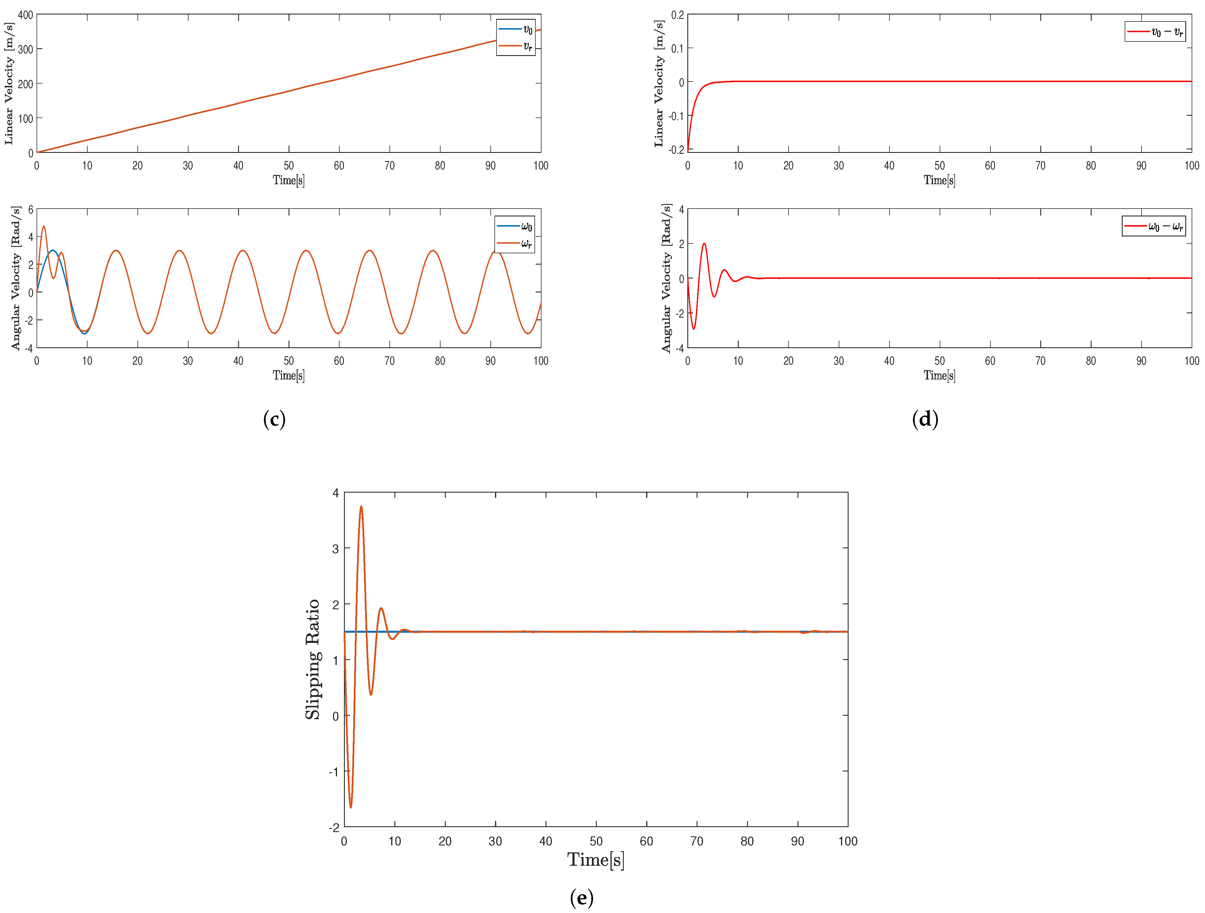Figure 4a illustrates the trajectory of $R_0$ and $R_r$. It is shown from Figure 4a that the $R_0$ can track the desired trajectory of $R_r$. Figure 4b indicates the tracking errors of $R_0$ converge to zero over time. Next, the linear and angular velocities of $R_0$ and $R_r$ using the controllers (30) are plotted in Figure 4c. Figure 4d, validates that the linear and angular velocity errors converge to zero. Figure 4e depicts the trajectory of the leader estimation of slipping ratio $\mu$ at 15 s.

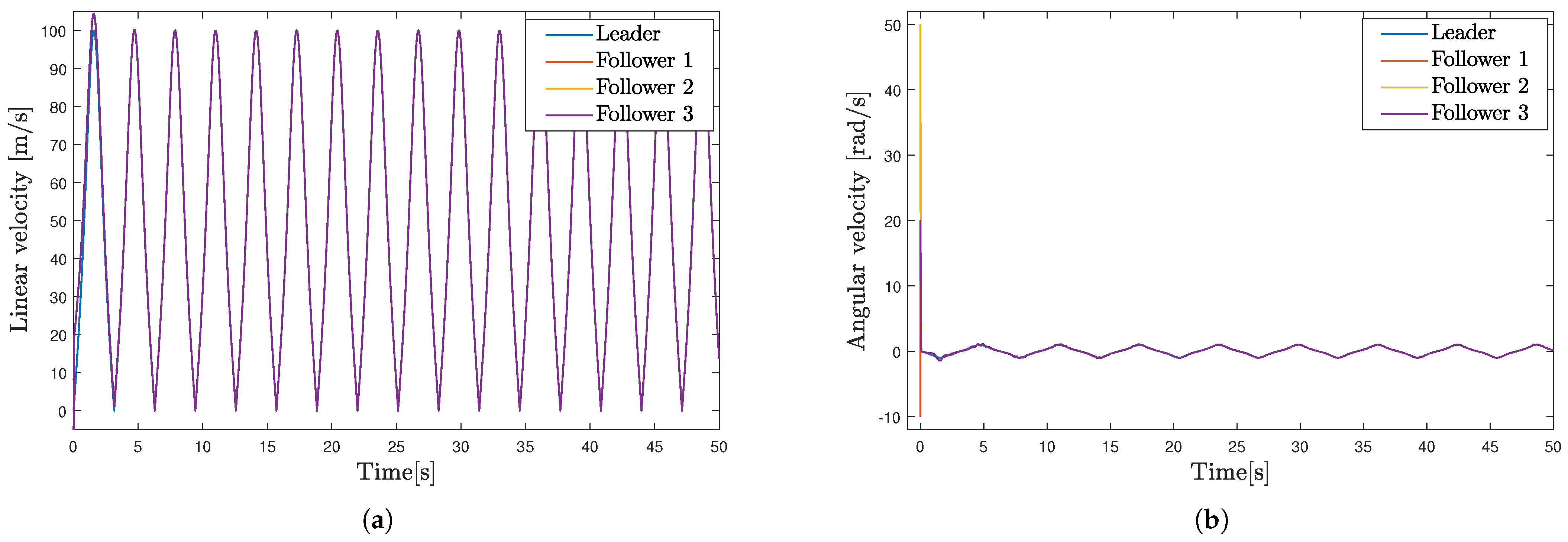
Part 2: As an illustration, the objective of our proposed method is a triangular formation. The angular and forward velocities of the leader NMR are given by ${\omega }_0=-{\displaystyle \frac{sint}{1+{(cost)}^2}}$ and $v_0=100\left|{\displaystyle \frac{sint}{1+{(cost)}^2}}\right|$. The initial values of the robots are set to $R_1\left(0\right)={[20,50,-5]}^T$, $R_2\left(0\right)={[-10,30,17]}^T$, $R_3\left(0\right)={[10,10,-15]}^T,R_0\left(0\right)={[10,30,0]}^T$. The desired relative position of $R_i$ are set as ${\mathsf{\Delta }}_{1x}=-40$, ${\mathsf{\Delta }}_{1y}=-10$, ${\mathsf{\Delta }}_{2x}=-80$, ${\mathsf{\Delta }}_{2y}=-30$, ${\mathsf{\Delta }}_{3x}=-40$, ${\mathsf{\Delta }}_{3y}=-50$. The parameters for estimation laws (48) and (49) are set to ${\kappa }_i=I_3$, ${\alpha }_1=800$, ${\beta }_1=20$, ${\alpha }_2=250$, ${\beta }_2=20$. The control law (72) and (73) parameters are set to $k_1=0.9$, $k_2=1.6$, $k_3=5$. We consider a group of four NMRs comprising three followers and one leader as shown in Figure 5.

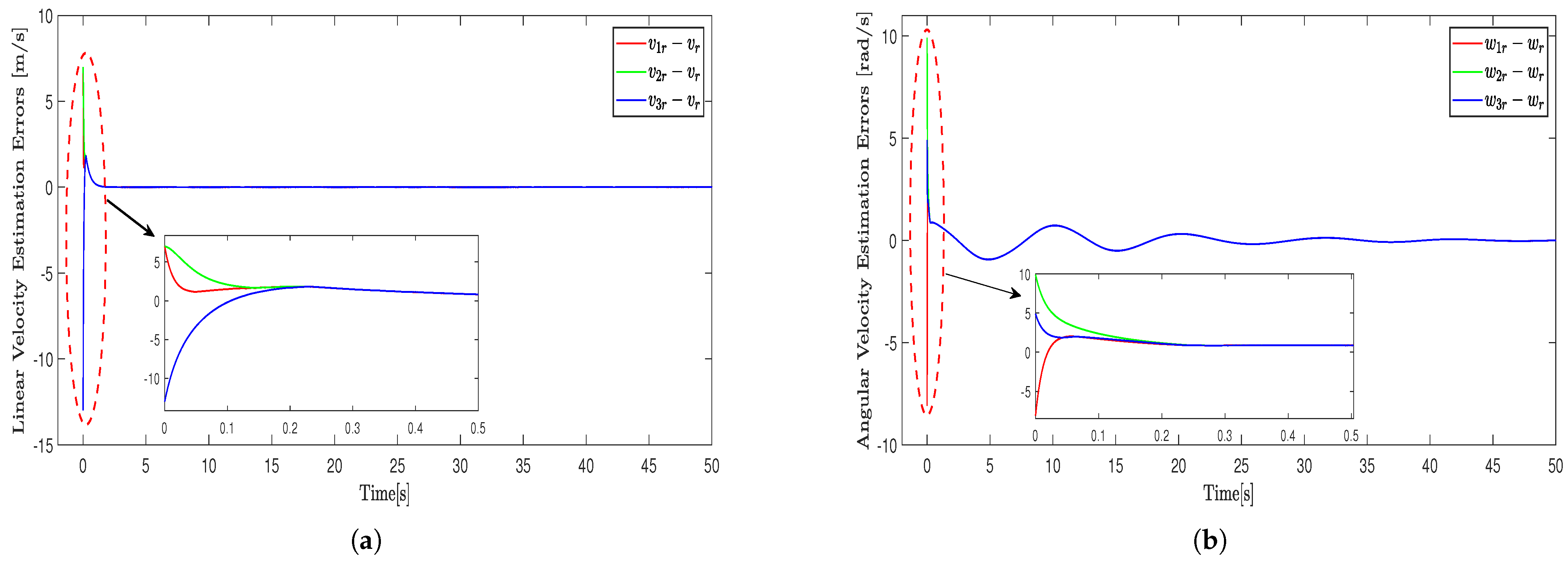
From Figure 6a,b the linear velocity estimation errors $(v_{ir}-v_r)$ and angular velocity estimation errors $({\omega }_{ir}-{\omega }_r)$ exponentially converge to zero.

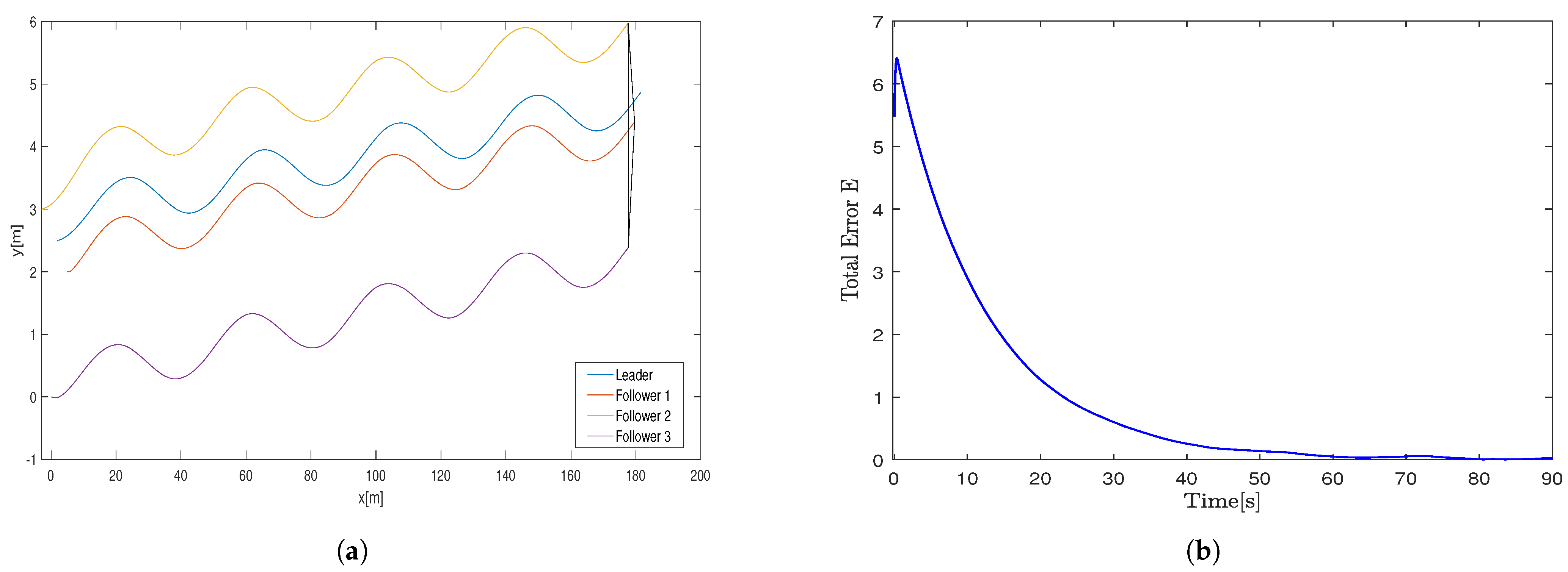
Figure 7a depicts the trajectories of all robots based on the observers and proposed control laws (72) and (73). Moreover, it is clearly seen from Figure 7a that the three follower NMRs follow leader $R_0$ converges to the desired formation. The proposed observer for each follower are displayed in Figure 7b, which estimates the relative position. The observer error trajectories are depicted in Figure 7c. On the other hand, from Figure 7d one can confirm the convergence of the formation tracking errors. 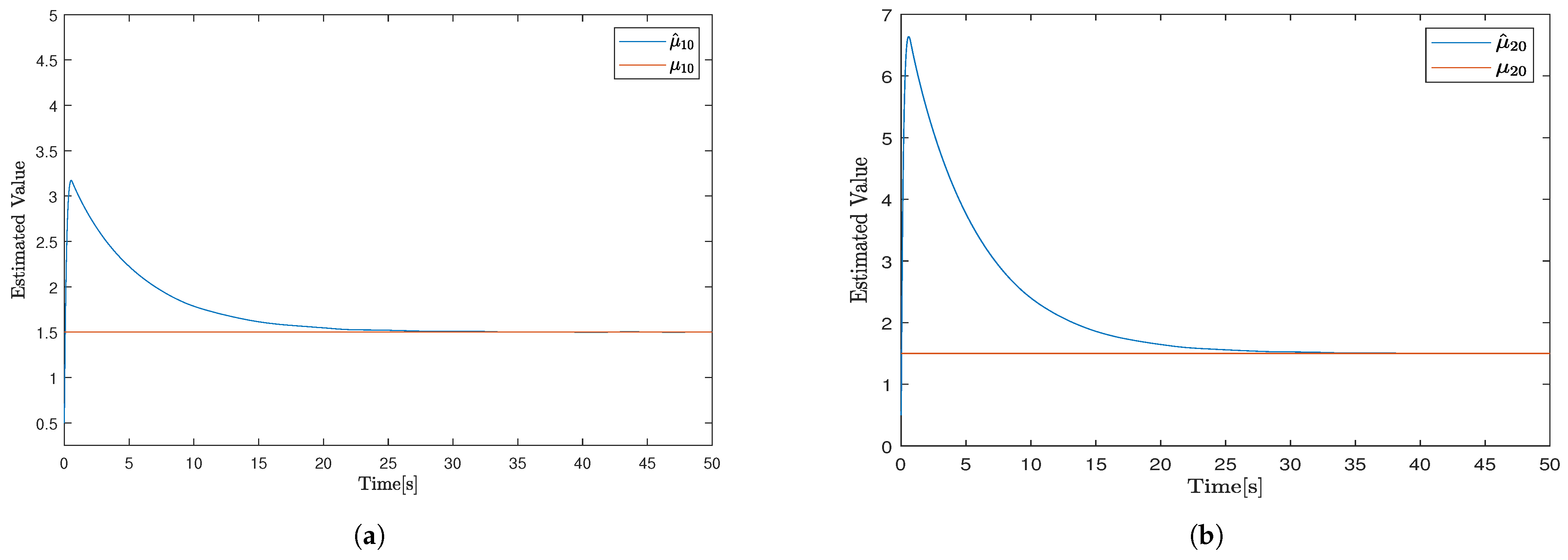Figure 8a,b depicts the adaptive estimation of slipping ratio ${\mu }_{10}$ and ${\mu }_{20}$ which converges to true value about 25 s. It demonstrate the gradual convergence of the estimated values ${[{\widehat{\mu }}_{10},{\widehat{\mu }}_{20}]}^T$ of unknown slipping ratios towards the true values ${[{\mu }_{10},{\mu }_{20}]}^T$. Moreover, the control inputs of the proposed method are displayed in Figure 9a,b. In order to demonstrate the effectiveness of the proposed algorithm, we consider more agents for the multi-robot formation. For this, we consider four follower NMRs along with a leader NMR to achieve rectangle formation. The results in Figure 10a describe the trajectories of NMRs where the desired rectangular formation is achieved. Subsequently, the formation tracking errors approach to zero with satisfactory performance. It can be seen that the intended formation shape is attained and then preserved using the proposed controller while following the leaders trajectory. As we can see from Figure 10b, five NMRs form the desired formation pattern under the distributed controllers (72) and (73) with directed interaction topology.

RMSE-Based Evaluation for Mobile Robot Formation Control: To quantitatively evaluate the performance of the mobile robot formation control system, we utilize the Root Mean Square Error (RMSE) metric. RMSE measures the deviation between the actual positions of the follower robots and their desired positions relative to the leader robot over time.

Let us consider the following: ${\mathbf{p}}_L\left(t\right)={[x_L\left(t\right),y_L\left(t\right)]}^T$: position of the leader robot at time t, ${\mathbf{p}}_i\left(t\right)={[x_i\left(t\right),y_i\left(t\right)]}^T$: position of the $i^{\mathrm{th}}$ follower robot at time t, where $i=1,2,3$, ${\mathbf{d}}_i={[d_{ix},d_{iy}]}^T$: desired relative offset of the follower i with respect to the leader, ${\mathbf{p}}_i^{\mathrm{desired}}\left(t\right)={\mathbf{p}}_L\left(t\right)+{\mathbf{d}}_i$: desired position of follower i.

The instantaneous position error of each follower is defined as:

$${\mathbf{e}}_i\left(t\right)={\mathbf{p}}_i^{\mathrm{desired}}\left(t\right)-{\mathbf{p}}_i\left(t\right)=\left({\mathbf{p}}_L\left(t\right)+{\mathbf{d}}_i\right)-{\mathbf{p}}_i\left(t\right)$$

(89)

The RMSE over a total of T time steps for all three followers is computed as:

$$\mathrm{RMSE}=\sqrt{{\displaystyle \frac{1}{3T}}\sum _{i=1}^3\sum _{t=1}^T{∥{\mathbf{e}}_i\left(t\right)∥}^2}$$

(90)

To evaluate the performance of the proposed distributed estimator-based formation control strategy, Root Mean Square Error (RMSE) metrics were computed for both the leader and follower mobile robots. In this study, a formation consisting of one leader and three follower robots was considered. The mobile robots are modeled as unicycle-type differential drive systems operating in a planar environment, and the objective of the control scheme is to enable the leader to track a predefined reference trajectory while the followers maintain desired relative positions with respect to the leader, thereby preserving the formation geometry during motion.

The proposed controller employs a distributed estimator mechanism, which allows each follower robot to estimate the leader’s state information (e.g., position and velocity) using only local sensing and limited communication with neighboring agents. This architecture enhances scalability and robustness, particularly in scenarios where centralized coordination is infeasible due to communication constraints or dynamic environments.

The RMSE between the leader robot and the reference trajectory was calculated to be 1.7571, indicating high accuracy in trajectory tracking by the leader under the proposed control law. For the follower robots, RMSE values were computed based on their deviations from the desired formation positions relative to the leader. Robot 2 achieved an RMSE of 2.7405, Robot 4 exhibited an RMSE of 3.0789, and Robot 3 showed the largest deviation with an RMSE of 4.3065. These results reflect the distributed nature of the control strategy, where estimation inaccuracies or local disturbances can cause slight variations in performance among the followers.

Despite these differences, all follower robots were able to maintain formation with acceptable errors, demonstrating the robustness and effectiveness of the proposed distributed estimator-based controller. The RMSE values also highlight the system’s ability to tolerate estimation and communication uncertainties, while still achieving coordinated group behavior. Further improvements in estimator accuracy or adaptive gain tuning could potentially reduce the observed variance in follower performance.

The results of the simulation experiments for trajectory tracking and formation maintenance under varying slippage conditions are summarized in

Table 1. RMSE of Trajectory Tracking Error Under Different Slippage Conditions.

Slippage Condition	W/o Adaptive Controller (m)	With Adaptive Controller (m)
No Slippage	0.12	0.11
Mild Slippage	0.45	0.18
Moderate Slippage	0.83	0.22
Severe Slippage	1.37	0.30

and

Table 2. RMSE of Formation Error Under Different Slippage Conditions.

Slippage Condition	W/o Adaptive Controller (m)	With Adaptive Controller (m)
No Slippage	0.10	0.09
Mild Slippage	0.38	0.15
Moderate Slippage	0.72	0.19
Severe Slippage	1.12	0.26

.

Table 1 presents the RMSE (Root Mean Square Error) for trajectory tracking performance with and without the adaptive controller. Under no slippage, the error is minimal for both controllers, with the adaptive controller slightly outperforming the non-adaptive one. As slippage severity increases, the tracking error grows significantly for the non-adaptive controller, while the adaptive controller maintains a much lower RMSE, demonstrating its effectiveness in compensating for wheel slippage.

Table 2 summarizes the RMSE for formation maintenance under different slippage conditions. Similar trends are observed: the adaptive controller consistently outperforms the non-adaptive one, especially as slippage severity increases. This indicates that the proposed adaptive control strategy significantly enhances the formation maintenance capability of the swarm in the presence of wheel slippage.

Overall, the adaptive controller significantly improves both trajectory tracking and formation maintenance performance, even under severe wheel slippage conditions, highlighting its robustness and effectiveness in real-world applications where such disturbances are common.

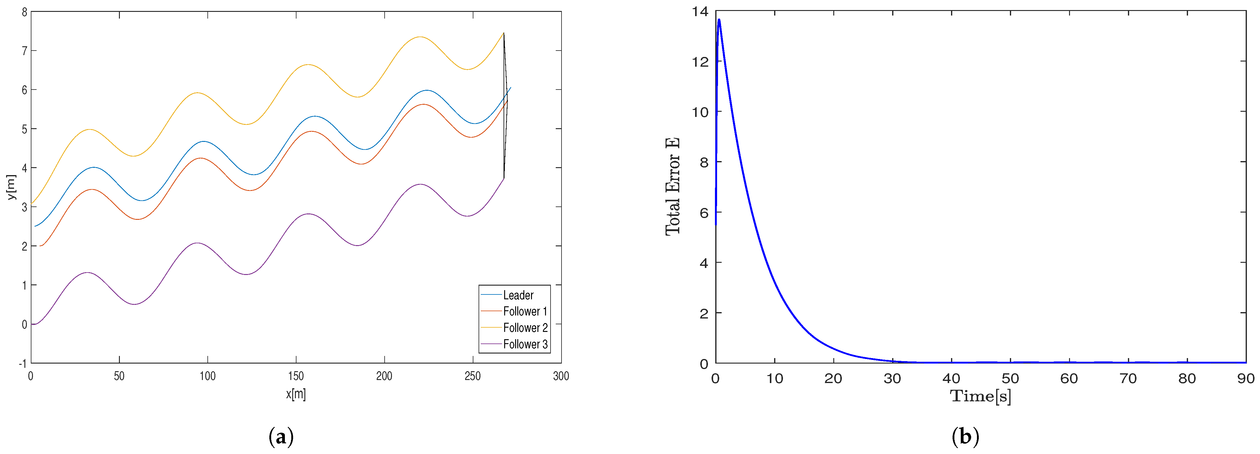
A comparative study is conducted against the control strategies proposed in [15,26] to demonstrate the advantages of the proposed formation control approach. In this evaluation, a leader–follower formation scenario is considered, consisting of one leader and three follower robots configured to maintain a triangular formation. To quantitatively assess the formation tracking performance, the total formation error is defined as follows:

$$\begin{array}{cc}\hfill E\left(t\right)& ={\left[\sum _{i=1}^3\left(|x_i\left(t\right)-x_r\left(t\right)-{\mathsf{\Delta }}_{ix}{|}^2+|y_i\left(t\right)-y_r\left(t\right)-{\mathsf{\Delta }}_{iy}{|}^2+{|{\theta }_i\left(t\right)-{\theta }_t\left(t\right)|}^2\right)\right]}^{{\displaystyle \frac{1}{2}}}.\hfill \end{array}$$

(91)

The performance comparisons among the controllers from [26], and the proposed method are illustrated in Figure 11, Figure 12 and Figure 13. For a fair comparison with the method in [15], the same simulation setup is used with controller parameters set as $k_1=0.01$, $k_2=0.5$, and $k_3=0.5$ in Equations (72) and (73). As shown in Figure 11, this method achieves strong performance; however, it is well-documented that the backstepping controller can induce large initial velocity magnitudes and sudden jumps in velocity under abrupt tracking errors, rendering it impractical for real-world implementation.

In contrast, the controller in [26] employs a distributed observer at each follower robot to estimate the leader’s state. The resulting robot trajectories using this method are presented in Figure 12, where the desired triangular formation is also attained. However, comparing the total error plots in Figure 12 and Figure 13, it is evident that the controller in [26] exhibits significantly larger errors during the initial seconds of operation. This degradation in performance is mainly due to the reliance on leader state estimates, which suffer from substantial initial estimation errors.

The proposed controller explicitly incorporates coordination errors between follower robots into its design, resulting in superior formation tracking accuracy. Unlike previous centralized approaches, the proposed method achieves formation control for wheeled nonholonomic mobile robots within a distributed framework. This marks a meaningful advancement, as distributed systems offer improved scalability, enhanced fault tolerance, and reduced computational and communication burdens on the leader robot. The simulation results further confirm that the proposed bio-inspired control model effectively addresses the velocity jump problem common in backstepping methods, thereby validating the efficacy of the proposed formation control strategy.

5. Conclusions

In this study, we have proposed formation tracking control for multiple robots based on distributed observers with slippage constraints. An adaptive controller has been implemented for the leader robot, enabling it to proficiently trace the reference trajectory even in the presence of slippage. Moreover, an individualized formation controller with distributed adaptability is devised for every subordinate robot, enabling the attainment of the desired formation goal despite encountering the impact of unfamiliar slippage. In particular, theoretical sufficient conditions have been derived based on a suitable Lyapunov-functional candidate. Finally, the correctness of the theoretical results has been verified by computer simulation where the proposed formation control scheme ensures the successful maintenance of the desired formation in the presence of unknown slipping effects. Future research should delve deeper into exploring robot communications, including topics such as denial of service attacks and noise interference, to enhance the accuracy of data transmission and improve control effectiveness in diverse conditions. Additionally, further investigation into obstacle avoidance is crucial to enhance the overall efficiency of formation control.