Estimation of Physical Stellar Parameters from Spectral Models Using Deep Learning Techniques

Abstract

This article presents a new algorithm that uses techniques from the field of artificial intelligence to automatically estimate the physical parameters of massive stars from a grid of stellar spectral models. This is the first grid to consider hydrodynamic solutions for stellar winds and radiative transport, containing more than 573 thousand synthetic spectra. The methodology involves grouping spectral models using deep learning and clustering techniques. The goal is to delineate the search regions and differentiate the “species” of spectra based on the shapes of the spectral line profiles. Synthetic spectra close to an observed stellar spectrum are selected using deep learning and unsupervised clustering algorithms. As a result, for each spectrum, we found the effective temperature, surface gravity, micro-turbulence velocity, and abundance of elements, such as helium and silicon. In addition, the values of the line force parameters were obtained. The developed algorithm was tested with 40 observed spectra, achieving $85\%$ of the expected results according to the scientific literature. The execution time ranged from 6 to 13 min per spectrum, which represents less than $5\%$ of the total time required for a one-to-one comparison search under the same conditions.

1. Introduction

Several works related to the use of techniques from the field of artificial intelligence in astronomy have been undertaken due to the high demand for processing, detection, and automated analysis of large amounts of data. It has become necessary to use machine learning techniques capable of modelling, detecting, predicting, or classifying events in real-time at observatories, or facilitating the analysis of data directly from the surveys [1,2].

This kind of study requires the production of artificial data, i.e., generated by simulations, theoretical models, and statistical experiments, among others. In the context of stellar parameters’ determination, we refer to theoretical spectra computed under physical assumptions and the radiative transfer process occurring in the stellar atmosphere, which is denominated stellar atmosphere models [3,4,5,6,7]. These simulated data of stellar spectra are used to deduce the physical parameters of the stars by comparing them to their respective observed spectra managed from different databases. This work uses machine learning techniques to develop a method that looks for the best representative model of an observed spectrum from a database containing many theoretical spectra.

We used the grid ISOSCELES (see Section 2.1), computed to analyse the stellar and wind properties of massive stars (approximately over 8 solar masses, $M\odot$) and, therefore, to study the important role that stellar winds have in the determination of mass-loss rates [8]. The challenge was to generate multiple comparisons between these models (also called synthetic spectra) with the real (or observed) stellar spectra, to deduce the parameters corresponding to the object under study. Therefore, the synthetic spectrum that best matches the real spectrum will be the one selected to determine the stellar and wind parameters.

During the last decades, the procedure for determining stellar parameters in massive stars has been refined generating a standard with excellent results [9,10,11]. However, substantial improvements in models of stellar atmospheres and the description of physical processes have further improved the estimation of such parameters [12]. In general, the procedure consists of a visual comparison of the observed spectral line profiles and their respective synthetic lines from the models. In the case of massive stars, the Balmer lines (hydrogen) are analysed in this process due to their great intensity, and their direct relation with gravity and stellar winds, together with the contribution provided by the helium lines. Through spectroscopic analysis in the optical range, it is possible to determine the following parameters: effective temperature ($T_{eff}$), surface gravity (log g), micro-turbulence velocity ($\zeta$), and abundance of elements, such as helium and silicon. In addition, particularly using the ISOSCELES spectral models, the values of the line-force parameters are obtained as follows: $\alpha$, $\kappa$ and $\delta$, where $\alpha$ is a ratio between the line force from optically thick lines and the total line force; $\kappa$ is related to the number of lines effectively contributing to the driving of the wind; and $\delta$ changes in the ionisation throughout the wind.

In this context, the challenge is summarised as finding the best spectral model for a real spectrum using the ISOSCELES grid, which has more than 573 thousand samples. In addition, each model has six variations according to the different values of the micro-turbulence velocities ($\zeta$). Due to the complexity of the problem, machine learning techniques were used to limit data processing and search times. Specifically, clustering and deep learning techniques were used for grouping data, since multi-layer neural networks manage to extract the main features of the data automatically and thus reduce the dimensionality of the problem [13,14,15].

In the literature, it is possible to find similar problems that have been addressed using deep learning techniques [16,17] as a solution to obtain good results, although for much narrower stellar parameter ranges ($T_{eff}$ [4000, 11,500] K; log g∈ [2, 5] dex) than those addressed in this work, and without considering the complexity of the wind hydrodynamic solutions for stellar models. Another case is reported in [18], where the authors succeeded in training long short-term memory type ANNs with the synthetic spectra produced by [19,20] covering the region of OB main-sequence stars in the H-R diagram. Different noise levels were added to the synthetic spectra to decrease the ANN sensitivity to observed spectra. However, the number of synthetic spectra used for training the ANN was 25,718, which is considerably lower than the 573,190 spectral models used in our work. Therefore, the level of granularity and resolution of stellar parameter estimation is less than for our method. Another recent method that used a recurrent artificial neural network is described in [21]. The proposed system was trained with 5557 synthetic spectra computed with the stellar atmosphere code CMFGEN that covers stars with the following stellar parameter ranges: $T_{eff}$ [20,000, 58,000] K; log g∈ [2.4, 4.2] dex; and stellar mass from 9 to 120 solar masses. On the other hand, autoencoder architecture techniques have been employed to reduce the dimensionality of the spectra projected in a new feature space [22]. After that, the algorithm transfers the learning to convolutional neural networks that finally determine the stellar parameters of M dwarf stars.

The main contributions of this paper are the following:

• In this article, we used a grid of spectral models comprising more than 500,000 samples. These models were created based on the first grid, which considers hydrodynamic solutions for the behaviour of stellar winds and radiative transport. As a result, our method produced stellar parameters with greater resolution and a better fit than other methods.
• The method we developed allows estimating parameters of massive stars in a relatively short time (between 6 and 13 min per observed spectrum). This represents less than $5\%$ of the total time required to compare the observed spectrum against each of the synthetic spectra in the grid (see exhaustive search method using the same data [23]). Therefore, the proposed method provided is much more efficient.
• Our method proposes a combination of deep learning, clustering, and supervised non-parametric learning (KNN) techniques to obtain the synthetic model that best fits a real stellar spectrum. The observed spectrum is represented in a latency space by an autoencoder neural network. It is then classified into clusters from this compact representation. Finally, the observed spectrum is compared with the synthetic spectra of the selected cluster using the KNN algorithm (specifically, the “Ball-Tree” algorithm). The architecture of this method is novel for the treatment of spectra and the estimation of stellar parameters in comparison with other proposed methods (e.g., [9,10,23]).

The remainder of the paper is organised as follows: Section 2 presents some context for the ISOSCELES grid and the work related to the development of a search algorithm; Section 3 describes the methodology and algorithm developed; Section 4 shows and discusses the experimental results of this research, and Section 5 presents the main conclusion and future work.

2. Background

2.1. Massive Stars and Their Winds

Massive stars (∼ over 8 M⊙) are continuously losing large amounts of material via their stellar winds, enriching the interstellar medium chemically and dynamically, and therefore affecting the evolution of the host galaxy [24,25,26,27]. The huge mass-loss rate from the star (e.g., a solar-type star typically loses ∼${10}^{-14}$ M⊙/year, while for massive stars, the mass-loss rate is about ∼${10}^{-6}$ to ${10}^{-8}$ M⊙/year) modifies its stellar evolution stages and hence the type of supernova remnant left [28,29]. In addition, stellar winds allow us to perform quantitative spectroscopic studies of the most luminous stellar objects in distant galaxies and thus enable us to obtain important quantitative information about their host galaxies. Observing the winds of isolated OBA supergiants in spiral and irregular galaxies provides an independent tool for the determination of extragalactic distances using the wind momentum–luminosity (WML) relationship [30,31,32]. To understand all these physical phenomena occurring in massive stars and all the impacts that they have in their surrounding media, we need to analyse spectroscopic (and photometric) observations at different wavelengths of different spectral and luminosity classes, and in different metallicity media, to cover all evolutionary stages of these stars. Currently, the theory that describes these winds (m-CAK theory) is based on the pioneering work of [33] and the improvements made by [34,35]. From the standard m-CAK theory, the line force parameters ($\alpha$, $\kappa$, and $\delta$) provide scaling laws for the mass-loss rate and the terminal velocity of the wind.

In addition, in recent years, observational data have dramatically increased, introducing the era of big astronomical data. Currently, thanks to the advent of multi-object spectrographs and multi-wavelength techniques, there are several observational projects, such as ESO-GAIA, APOGEE (SDSS), POLLUX, IACOB, VLT-FLAMES Tarantula survey, and LAMOST, collecting and storing huge quantities of stellar spectra. Moreover, the analysis of spectral lines is performed by stellar atmosphere model comparison, using models that have been improved over the years. Therefore, it has become necessary to develop efficient analysis tools to use the models and compare them with observations, since this task is no longer possible by human interaction.

2.2. ISOSCELES Grid

ISOSCELES, GrId of Stellar AtmOSphere and HydrodynamiC ModELs for MassivE Stars, is the first grid of synthetic data for massive stars that involves both the m-CAK hydrodynamics (instead of the generally used $\beta -law$) and the NLTE radiative transport [36].

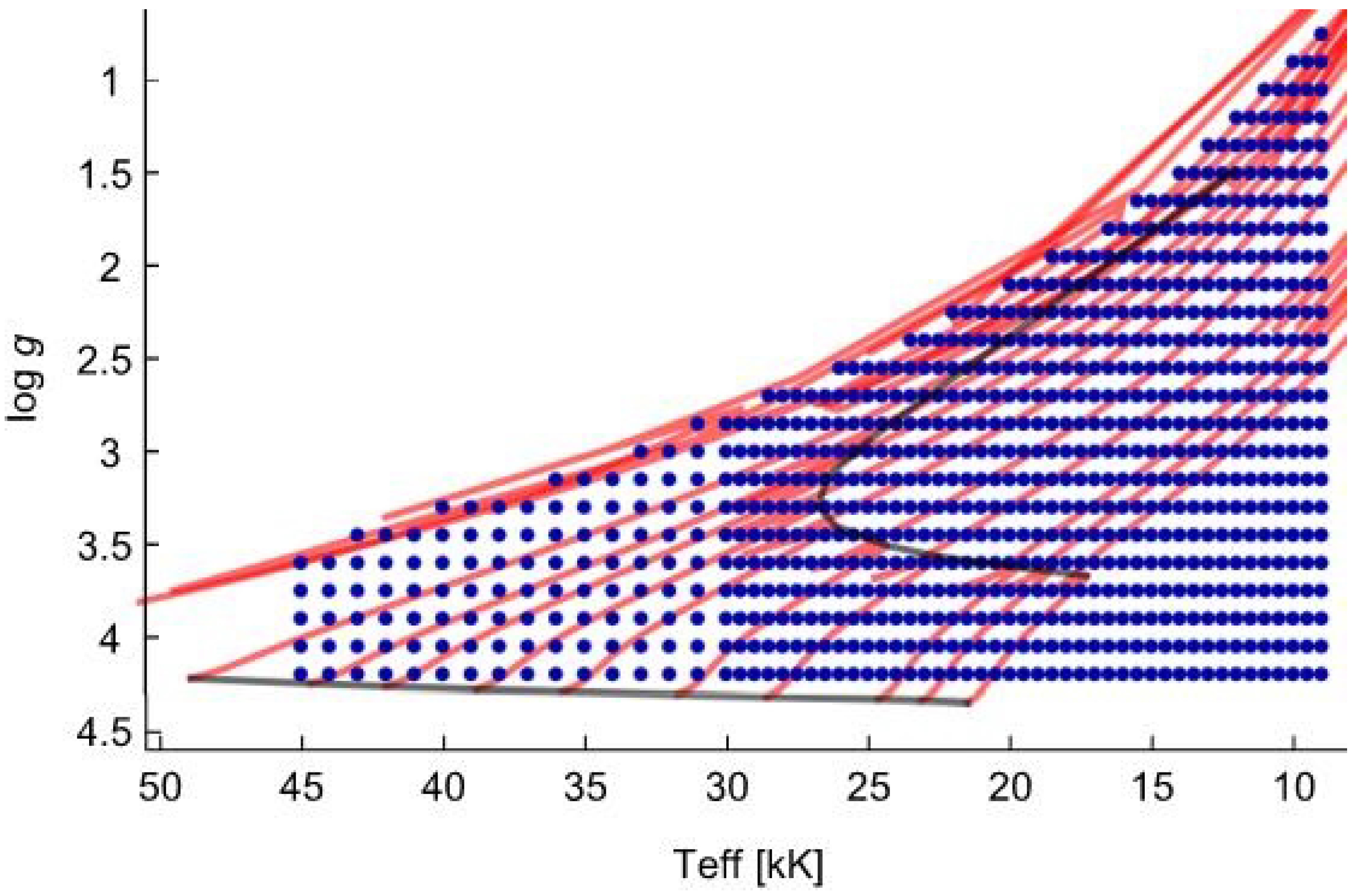
ISOSCELES covers the complete parameter space of O-, B-, and A-type stars. To produce a grid of synthetic line profiles with the code FASTWIND, we first computed a grid of hydrodynamic wind solutions with the stationary code HYDWIND. The surface gravities comprise the range of $log g=4.3$ down to about $90\%$ of the Eddington limit in steps of $0.15$. We consider 58 effective temperature grid points, ranging from 10,000 [K] to 45,000 [K], in steps of $500\left[\mathrm{K}\right]$ below $30,000\left[\mathrm{K}\right]$ and in steps of 1000 [K] above it.

Therefore, the grid points were selected to cover the region of the $T_{eff}-log g$ diagram (Figure 1), where the O-, B-, and A-type stars are located from the main sequence to the supergiant phase.

Although we focused on the study of B- and A-type stars, we have implemented a wide grid for further analysis and to avoid observed stars too close to the grid’s borders. Each HYDWIND model is described by six main parameters: $T_{eff}$ (effective temperature), $log$ g (log of gravity), $R_{*}$ (stellar radius), $\alpha$, $\kappa$, and $\delta$. All these models consider the boundary condition for the optical depth, ${\tau }_{*}=2/3$, at the stellar surface. For each given pair ($T_{eff}$, $log g$), the radius was calculated from $M_{bol}$ by means of the FGLR [38,39]). Note that this relationship was observationally established for supergiant stars, but we have also used it for models that represent stars that do not belong to this luminosity class. However, this calculation of the radius does not affect the analysis because it will be derived in the final step of the analysis. The range of line force parameters is given in

Table 1. Combinations of the line-force parameters for the grid of hydrodynamic models.

P	Values
$\alpha$	0.45 0.47 0.51 0.53 0.55 0.57 0.61 0.65
$\kappa$	0.05 to 0.60 (step size of 0.05)
$\delta$	0.00 0.04 0.10 0.14 0.20 0.24 0.26 0.28 0.29 0.30 0.31 0.32 0.33 0.34 0.35

, where the values of $\delta$ are necessary to obtain both fast and $\delta -slow$ solutions. It is worth noting that not all combinations of these parameters converge to a physical stationary hydrodynamic solution.

We used H, He, and Si atomic lines to derive the photospheric properties of the star and the characteristics of its wind. In our case, each FASTWIND model is described by seven main parameters: $T_{eff}$, $log$ g, $R_{*}$, $v_{\infty }$, $\dot{M}$, $log{\epsilon }_{Si}$, and $v_{micro}$ (note that the first five parameters were calculated in the hydrodynamic part of this methodology). For calculating the NLTE model atmospheres, we used micro-turbulent velocities of 8, 10, and 15 [km/s] for temperature ranges $T_{eff}<15,000\left[\mathrm{K}\right]$, $15,000\left[\mathrm{K}\right]<T_{eff}<20,000\left[\mathrm{K}\right]$ and $T_{eff}>20,000\left[\mathrm{K}\right]$, respectively, whereas for all synthetic line profiles (from all models) micro-turbulent velocities ($\zeta$) of 1, 5, 10, 15, 20, and 25 [km/s] were used. For silicon abundances ($log{\epsilon }_{Si}$), we adopted five different values: $7.21$, $7.36$, $7.51$ (solar), $7.66$ and $7.81\left[\mathrm{dex}\right]$. The abundance of helium was fixed to the solar value $He/H=0.10$. The actual radius should be determined from the visual magnitude, the distance of the star, and its reddening. The grid was transformed from ASCII to binary format (FITS) to reduce its size. In total, we obtained 573,433 synthetic spectra with a size of 289 [Gb] (FITS format). Currently, part of our grid ISOSCELES is publicly available at https://www.ifa.uv.cl/grid (accessed on 10 August 2024).

Considering the huge amount of observational data and the half million models from ISOSCELES, there is a necessity to develop new computational methods to determine the best model that reproduces the observed spectra, and to determine the stellar and wind parameters and the evolutionary state of the stars, their chemical composition, and many other characteristics.

2.3. Related Work

In the context of a master’s thesis, during the year 2022, the study “Analysis of the momentum–luminosity relationship in massive stars” was presented, which, in turn, presented the development of an exhaustive search algorithm for spectral models belonging to ISOSCELES [23]. Regarding the algorithm, before being executed, it requests the entry of data of the profiles of six spectral lines of the star that need to be analysed, these are as follows: H$\gamma$, He I4471, Si III4552, H$\beta$, H$\alpha$, and He I 6678. In addition, the rotational parameters of the star vsini and $v_{macro}$ are required with which the synthetic spectra will be convolved, simulating line broadening due to stellar rotation. Furthermore, and optionally, it is possible to enter expected values of $T_{eff}$, $log$ g, and type of solution ($fast$ or $\delta$-$slow$), and to set an offset $\Delta \lambda$ of each line. The latter is because the lines are formed in different parts of the photosphere, so they usually present small shifts in wavelength. The optional data help narrow the search areas for spectral models in the grid, so they depend on the user’s knowledge of the stellar object under study. The lack of such optional information implies that the algorithm uses all grid models in the search process.

This code was tested on a multiprocessing server, where in each search, the loads, interpolation, and convolution of the spectral models are performed in parallel by each processor. Synthetic lines are compared with the observed spectral lines by ${\chi }^2/6$ (6 for the number of lines). The algorithm stores in a search list all spectral models with ${\chi }^2/6$ less than 1.0. Finally, it sorts the results in ascending order, selecting the best spectral model for the analysed star based on the lowest value of ${\chi }^2/6$ from the list. In summary, the processing times of the algorithm will depend on the expected parameters that are optionally entered before execution. The result was obtained of times from 5 to 10 min, when all possible optional parameters were delivered, and of 240 min, when no optional parameter was delivered.

As this work represents a first approach to the development of an algorithm that facilitates searches for ISOSCELES spectral models, the results obtained here will be used for comparison, including the same observed spectra and their lines managed from the same database.

3. Proposed Approach

3.1. Methodology

The grid method is a viable solution to the problem of obtaining the main parameters of a star from spectroscopic analysis. In this case, the technique is difficult to use because it is challenging to find the best synthetic spectrum within a grid of 573,433 models. Therefore, to address this task using efficient search algorithms, this paper proposes to address the problem with deep learning, clustering, and machine learning techniques. In this way, the trained classification models can narrow down the search regions and, therefore, the time involved in the process.

Before detailing the methodology, we note that it was necessary to eliminate erroneous synthetic spectra from the grid. Line profiles with physically impossible results were detected, which were excluded from the analysis. After data cleaning, the number of spectral models was reduced to 573,190.

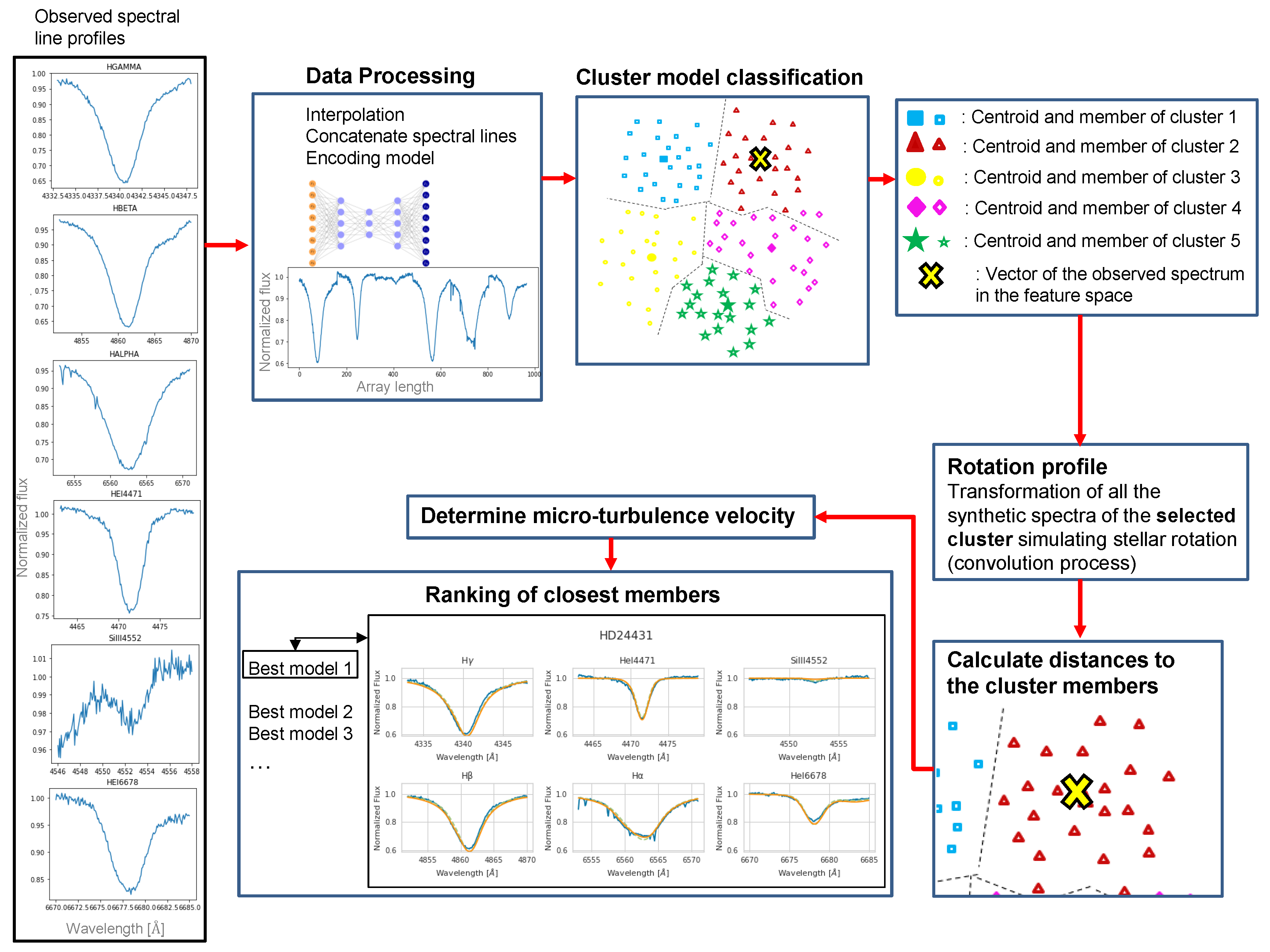
The proposed methodology consists of a strategy focused on training clustering models on the synthetic spectra reduced to only six line profiles. This produces an advantage in the search process since, by classifying a real spectrum in one of the clusters defined by the model, the number of synthetic spectra with which it must be compared is reduced. The developed method has a data preprocessing step (see Section 3.1.1). This includes coding spectral models using an autoencoder to facilitate cluster modelling (see Section 3.1.2). After the classification of the observed spectra (see Section 3.1.3), it is necessary to apply stellar rotation transformations on all the synthetic spectra of the selected cluster, through a convolution process (see Section 3.1.4), according to the velocity parameters of the analysed star. This last process helps to generate a detailed comparison of each of the spectral lines, since in this way, all the spectra are affected by the same line broadening due to stellar rotation. Thus, the comparison mechanism of the real spectrum vs. the individuals in the cluster is determined by the KNN algorithm (see Section 3.1.5). Finally, when the search algorithm is fully processed, the result is a ranking of spectral models that best fit the real spectrum according to a distance metric (see Section 3.1.7), in addition to the comparative plots of the best model with the observed spectrum (see scheme in Figure 2).

3.1.1. Generating Feature Vector of Spectral Models

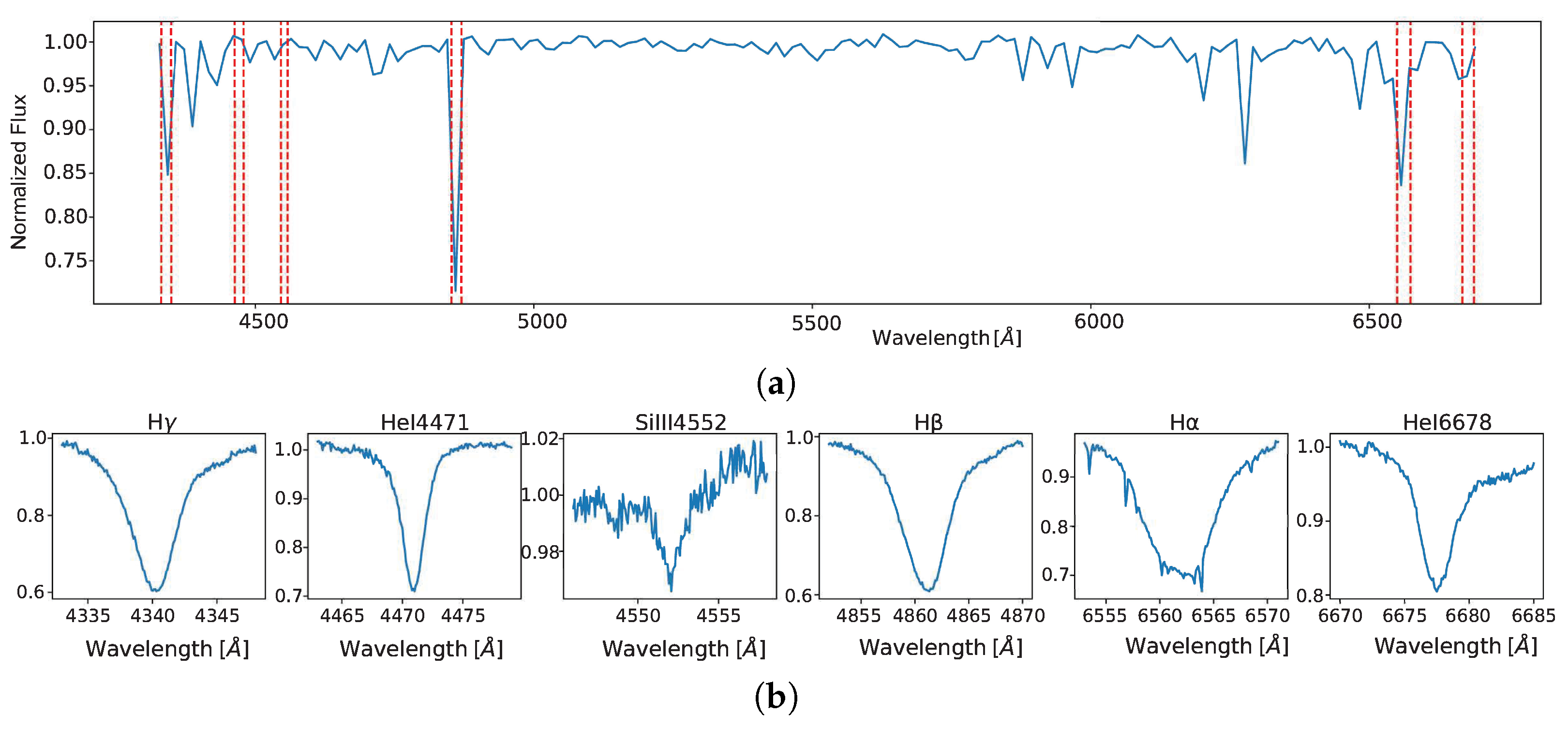
The wealth of information that grid models possess is fundamental to spectral analysis. However, not all of it has the same value if we focus on an efficient search strategy. For this reason, we propose to select only six spectral lines from each of the models, which have been used in different studies of massive stars [23,40,41] because of their direct relationship with the main parameters of this type of object. These are (in ascending order according to their wavelength) as follows: H$\gamma$, He I ($4471\AA$), Si III ($4552\AA$), H$\beta$, H$\alpha$, He I ($6678\AA$) (see

Table 2. Wavelength range of spectral lines selected to estimate stellar parameters.

Spectral Line	Wavelength [Å]	Wavelength Range [Å]
$H\gamma$	4340	4333–4348
$HeI4471$	4471	4463–4479
$SiIII$ 4552	4552	4545–4560
$H\beta$	4861	4852–4870
$H\alpha$	6563	6553–6571
$HeI$ 6678	6678	6670–6685

and Figure 3). It is common to observe in massive stars high-intensity Balmer lines, which are a useful source of information to determine stellar gravity and parameters related to stellar winds. The He I and Si III lines allow us to determine the effective temperature and abundance of these elements. Thus, the complexity of the spectral models is reduced to their representation of only six line profiles, which for analysis purposes are concatenated considering a specific wavelength range for each of them (see Table 2). Each spectral model is a vector of length 966 since per line profile, 161 points are considered, where these are represented in a 966-dimensional feature space. In addition, it is necessary to interpolate the lines so that their points are equidistant.

Another way to simplify the problem is by selecting all spectral models with a default value of $\zeta$, corresponding to 15 [km/s]. Each spectral model contains six versions according to different values of $\zeta$, specifically: 1, 5, 10, 15, 20, 25 [km/s]. All these versions of the same model have negligible variations compared to other models. However, the correct $\zeta$ value will be determined in the process of selecting the models closest to the observed spectrum (see Section 3.1.6).

3.1.2. Coding of Spectral Models

For the developed method, it is proposed to use deep learning techniques to extract features from the concatenated lines. Therefore, the dimensionality of the feature vectors, which represent each spectral model, is reduced. The type of ANN selected for this work is “autoencoder”, which is ideal for this type of problem where the data are not classified. Therefore, the ANN was trained to reproduce the input data based on their encoding and decoding, minimising the dimensionality in the central layer (bottleneck). In this way, a compact representation of the input data is obtained [14].

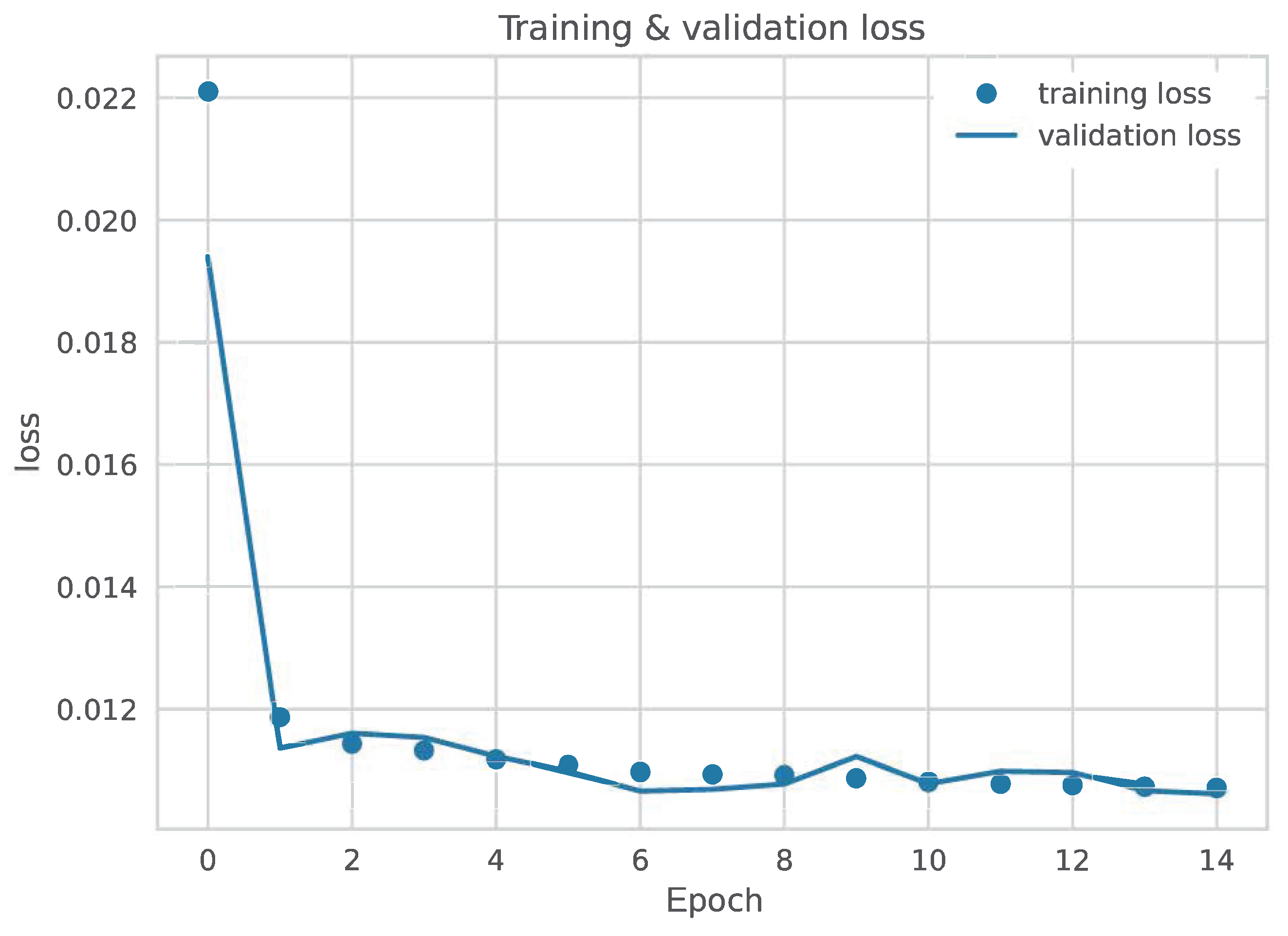
The best-performing ANN architecture is detailed in

Table 3. Autoencoder ANN architecture for training.

Layer	Type	Number of Neurons	Number of Parameter
Input	Input Layer	966	0
Layer1	Dense	1024	990,200
Layer2	Dense	512	524,800
Layer3	Dense	256	131,328
Bottleneck layer	Dense	12	3004
Layer4	Dense	256	3328
Layer5	Dense	512	131,584
Layer6	Dense	1024	525,312
Output Layer	Dense	966	990,150

, where the encoding layers (L. 1, 2, and 3) and decoding layers (L. 4, 5 and 6) decrease and increase in the number of neurones, respectively. The training parameters are detailed in

Table 4. Training parameters in ANN autoencoder.

Parameter	Value
Trained parameters	3,299,794
Epochs	15
Batch size	32
Loss function	MSE
Training data	$80\%$
Validation data	$20\%$

, while the plots of the loss function results for the training and validation data are seen in Figure 4. Finally, the encoder model is configured to receive input data and this returns the values of the bottleneck layer.

3.1.3. Clustering Model

Regarding the clustering method, it was proposed to use the synthetic spectra in their compact representation as a product of processing them using the trained autoencoder model (see Section 3.1.2). This was to train the cluster model with the encoded spectra and in this way group them according to their main characteristics. The K-Means algorithm was used, where the centroids were randomly initialized.

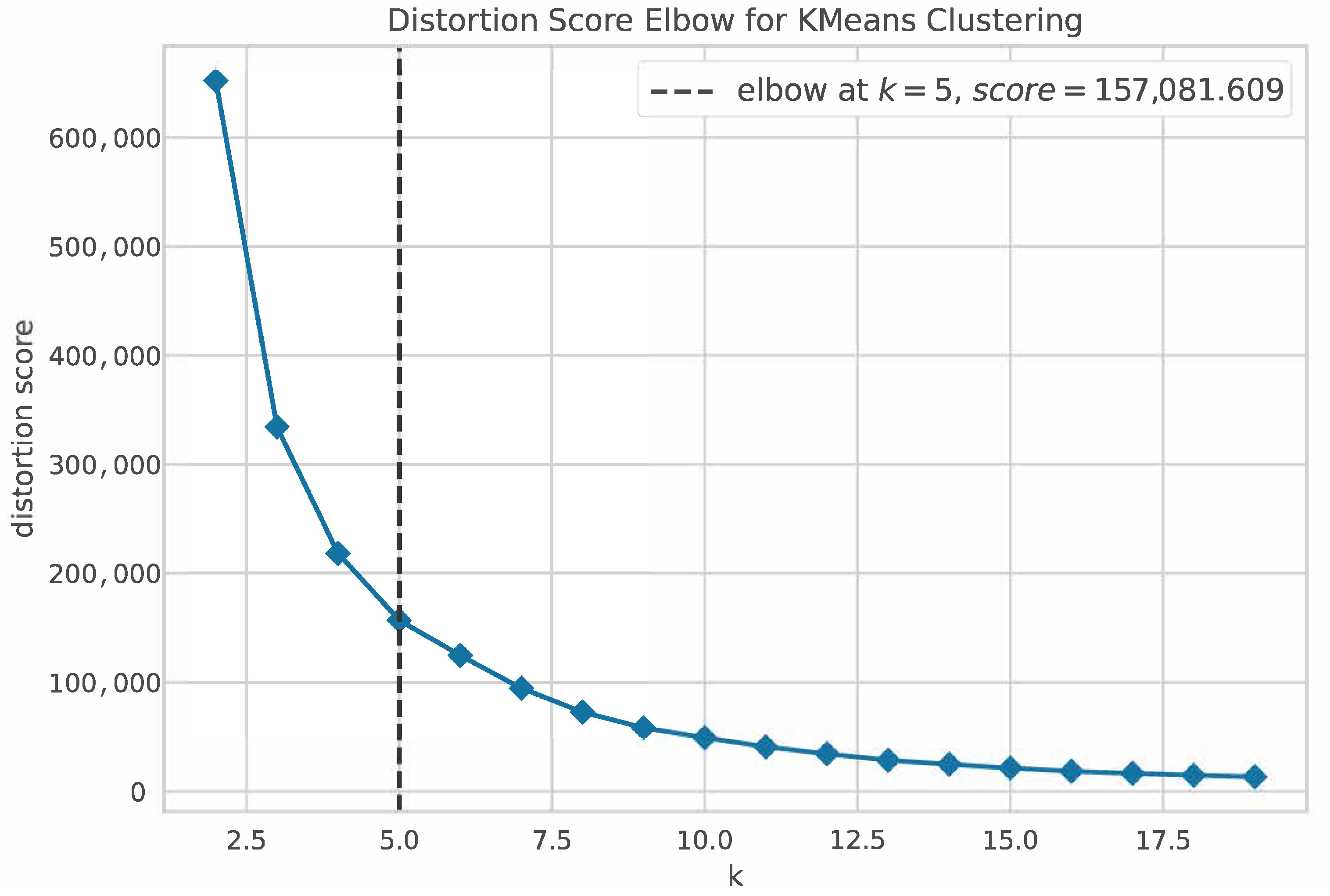
To obtain the optimal number of clusters that group the synthetic spectra, the “elbow method” was used, which consists of executing the clustering algorithm for different numbers of clusters that group the universe of individuals. Subsequently, the number K of clusters with which the algorithm was run is plotted against the respective inertia criterion calculated for each of these clusters. Finally, the value of K is chosen according to the inflexion point in the plotted curve as this value reveals that the increase in K does not represent a substantial change in the intra-cluster variance (see Figure 5). The inflexion point of the curve is calculated by the function of Equation (1) [42]. Therefore, the quantity of the cluster $K=5$ is determined to be the optimum for the synthetic spectra encoded by the autoencoder model.

Table 5. Distribution of spectral models in 5 clusters.

Cluster	Number of Individuals
0	155,088
1	88,556
2	95,785
3	194,812
4	38,949

details the number of individuals per cluster.

The number of iterations performed by the K-Means algorithm to declare the convergence of the model was 17. That is, the number of iterations necessary for the difference between a centroid and its new position in the next iteration to be less than a tolerance value for this work was defined as follows: tolerance = 0.0001.

$$K_f\left(x\right)={\displaystyle \frac{f^{″}\left(x\right)}{{(1+f^{\prime }{\left(x\right)}^2)}^{1.5}}}$$

(1)

3.1.4. Transformation of Synthetic Spectra

After the classification process of a real spectrum using the trained cluster model, all members of the selected cluster must be transformed. The feature vectors are (approximately) in the same conditions as the real spectrum, and in this way, they can be compared and distances between them can be measured.

The transformations consist of applying line broadening simulating stellar rotation effects using a convolution process and constraining the spectral lines to the same wavelength ranges entered for the real spectrum. For the convolution process, the velocity parameters ($vsini$ and $v_{macro}$) of the star studied are used, which are determined by the iacob_broad tool [43], available at http://research.iac.es/proyecto/iacob/pages/en/useful-tools.php (accessed on 10 August 2024). The IACOB project-Useful Tools.

3.1.5. Distances to Spectral Models

For the calculation of the distances between the observed spectrum and the synthetic spectra of the cluster selected by the model, the supervised learning algorithm “NearestNeighbors” (from scikit-learn) was used, which acts as an execution intermediary for three algorithms that calculate distances to near neighbours. These algorithms are as follows: “K-D Tree”, “Ball Tree”, and “Brute force”. For this work, “Ball Tree” was chosen due to its computational efficiency for feature vectors with a high number of dimensions (966 for this work). The strategy of this algorithm is to partition the data into a series of nested hyperspheres, generating a tree map of hyperspheres. Each of these is defined by a centroid and a radius; therefore, each point within the hypersphere will be defined by the same centroid as this one and a radius less or equal to that of the hypersphere. Finally, the distance calculation between a test point and a centroid determines the distance limits (upper and lower) to all points within the node [44].

Regarding the metric used for the calculation of distances, this is the “Euclidean distance”, which is defined in Equation (2) in its general form (Minkowski), where $p=2$.

$$D(X,Y)={\left(\sum _{i=1}^n{|x_i-y_i|}^p\right)}^{1/p}$$

(2)

3.1.6. Determining the Micro-Turbulence Velocity

In this process, 100 spectral models nearest to the real spectrum entered into the search algorithm are selected, and from these, all values of $\zeta$ are loaded directly from the ISOSCELES grid. Therefore, for each spectral model, there are 6 versions according to different values of $\zeta$, and line-broadening transformations are applied according to the rotational velocity parameters of the analysed star.

3.1.7. Best Spectral Model

Finally, a ranking of models nearest to the real spectrum is determined by the KNN algorithm described in the previous section, including results of the calculated Euclidean distance, and plots of the observed and synthetic spectral lines. In addition, the algorithm provides fast and $\delta -slow$ solutions for comparison.

4. Experimental Results

4.1. Data Acquisition

The observed spectra selected to analyse and test the developed algorithm correspond mainly to the dataset that was used in the masterwork of [23]. This research uses the ISOSCELES spectral model grid to make the comparisons using an exhaustive search algorithm. The objective is to compare the search times and efficiency of the algorithm developed in this work, together with the validation of the results. For this reason, the same six spectral lines and wavelength-shift values have also been used for analysis.

The observed spectra used in this work come from two databases. The first set of spectra was captured by the REOSC spectrograph, installed on the Jorge Sahade telescope (2.15 m in diameter) at the “El Leoncito” Astronomical Complex (CASLEO), located in San Juan, Argentina. On the other hand, the second group of spectra comes from the IACOB database, which is part of a scientific contribution project in the study of massive stars, where large amounts of spectra and photometry, among other empirical data, have been made freely available at: http://research.iac.es/proyecto/iacob/pages/en/introduction.php (accessed on 10 August 2024). The spectra were collected from the “Roque de los Muchachos” Observatory (ORM) located in La Palma, Spain.

4.2. Input Data Specification

When inputting the spectral data of the star into the search algorithm, the wavelength ranges of each line profile must be specified, which must be less than or equal to the ranges considered for the synthetic spectra with which the classification models were trained (see Table 2). However, all the line profiles of the observed spectra presented a smaller wavelength range, since this avoided considering ranges where noise present in the line continuum is included.

Other data that must be entered are the wavelength shifts of each spectral line, since these are formed in different parts of the photosphere. In this way, it will be possible to correctly visualise the comparison of the spectral lines with their respective models selected by the search algorithm.

4.3. Technical Processing Data

The algorithm development is written in Python version 3.10. The hardware dedicated to processing the algorithm is a 64-processor server, with 126 [Gb] of RAM, plus a swap memory of 1 [Gb]. This amount of available memory is necessary to run the algorithm as the feature vectors of all spectral models must be loaded into the run-time environment together with the clustering models, coding, and name list of each synthetic spectrum, which commits approximately 35 [Gb] of memory in total. To simplify this process, all the data required for loading are stored in serialised objects using functions from the “Pickle” library. The total data loading time is approximately 16 min.

However, running the algorithm involves using between 60 and 80 [Gb] of additional memory, depending on the number of individuals in the sorted cluster. The convolution and loading processes of the closest models with all their $\zeta$ values are distributed over 30 processors running in parallel, which speeds up the process, but at the same time requires a large amount of available memory.

4.4. Algorithm Execution and Results

The real stellar spectra were processed one-by-one; the algorithm is detailed in Section 3.1.3, whose execution times are detailed in

Table 6. Algorithm execution time according to cluster. The remaining clusters were not selected by the model for the tested spectra.

Cluster	Average Execution Time [min]
0	11
1	7
2	6
3	13

, which are dependent on the number of individuals in the classified cluster.

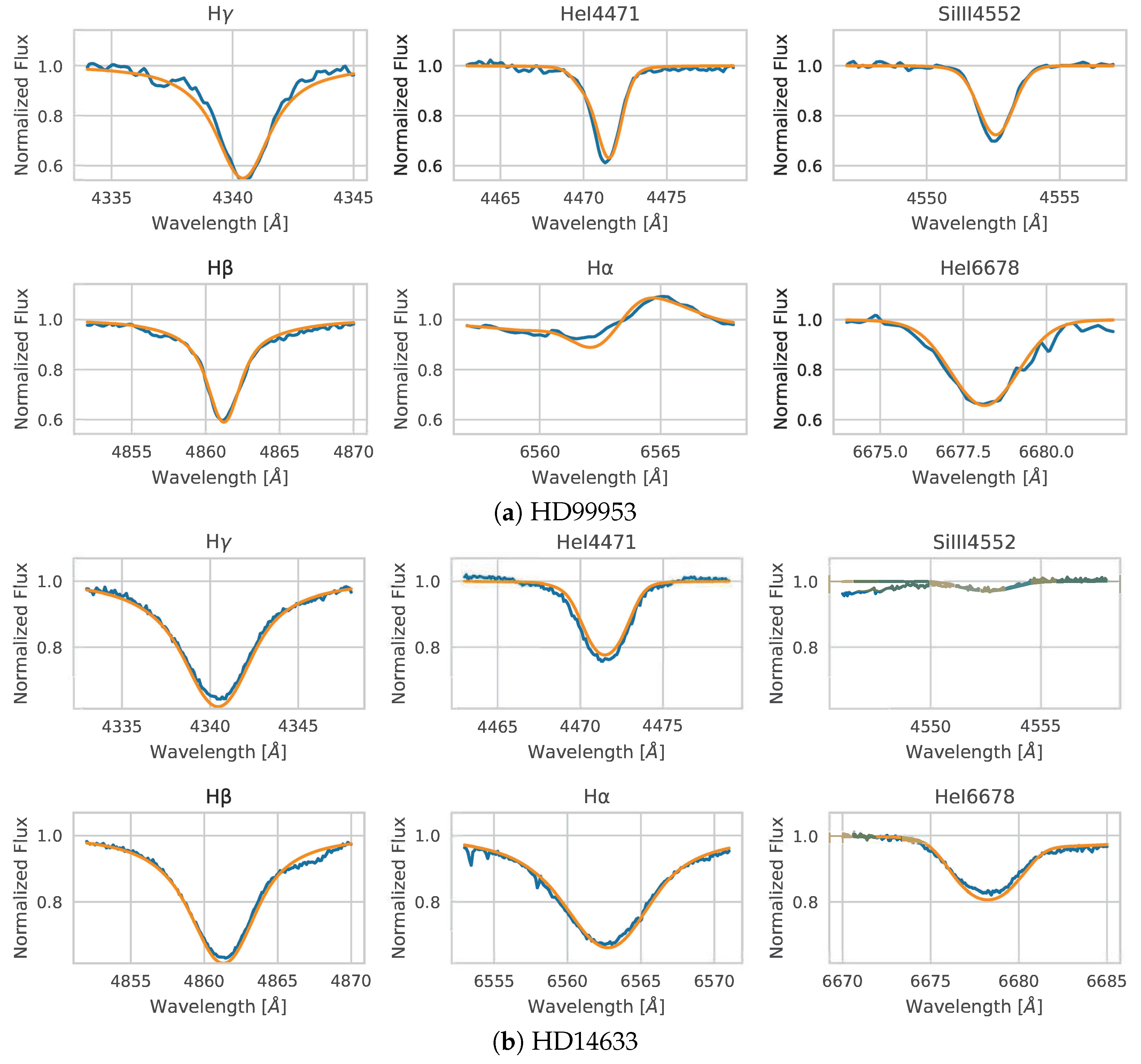
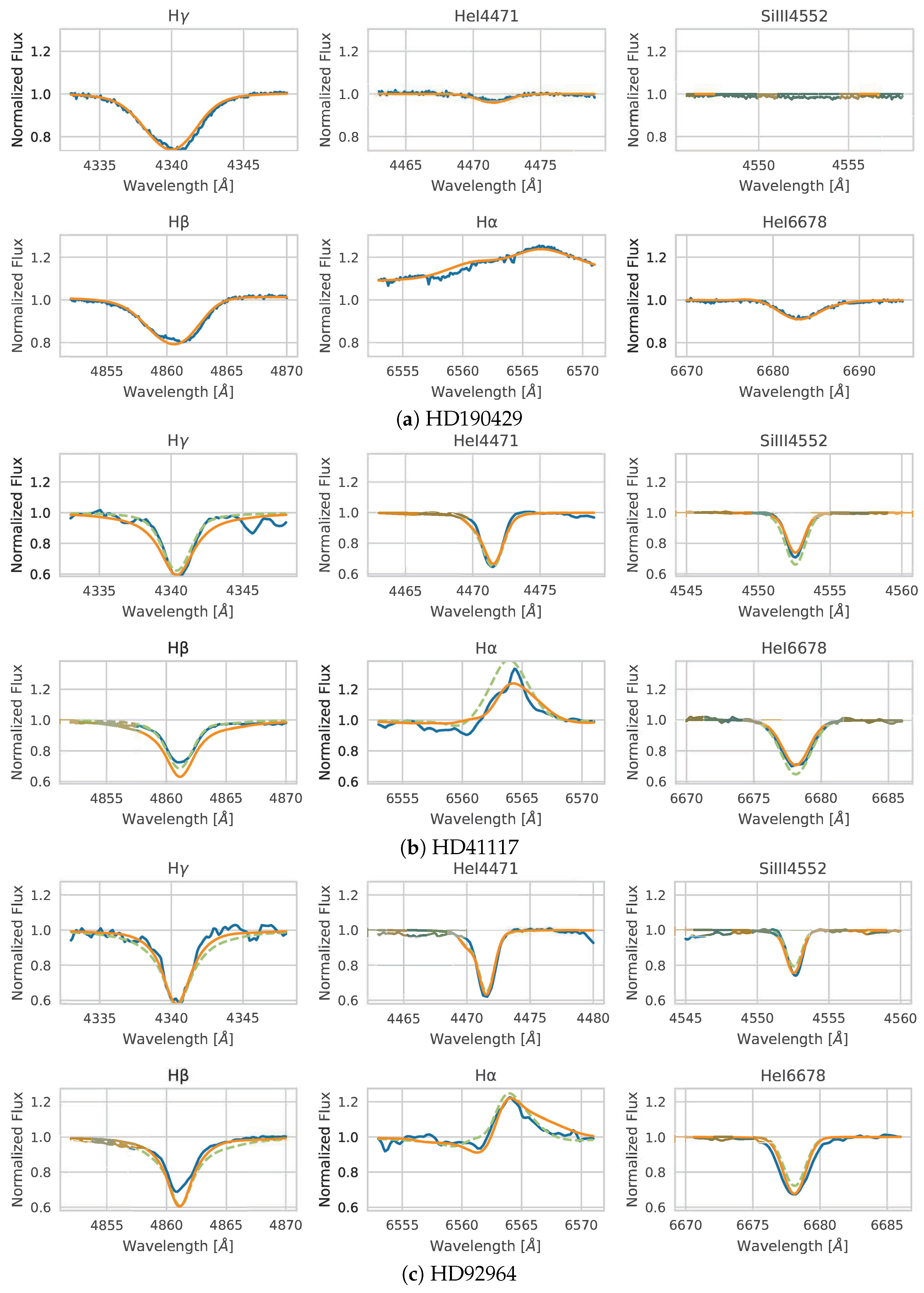
Figure 6 and Figure 7 show some results of comparative plots as examples, where the observed spectra (blue curve) entered into the algorithm and their respective spectral models obtained (orange curve) are shown. In addition, the best model found by the exhaustive search algorithm of [23] can be seen (segmented green curve) as a comparison, though for the cases where the same results were obtained, the latter is not shown.

Table 7. Stellar parameters of the nearest spectral models to each observed spectrum. In red are the cases where the spectral models have parameters unexpected according to previous studies (see column “Ref.”), where ED is the Euclidean distance (Equation (2)), and ED* is the Euclidean distance calculated to the spectral model found in [23].

Obj. HD	Sol. Type	${\mathit{T}}_{\mathit{eff}}$ $\left[\mathbf{K}\right]$	log g $\left[\mathbf{dex}\right]$	$\mathit{\alpha }$	$\mathit{\kappa }$	$\mathit{\delta }$	$\mathit{log}$ Si	$\mathit{\zeta }$ $\left[\frac{\mathbf{km}}{\mathbf{s}}\right]$	ED	ED*	Ref.
99,953	$\delta$-s	18,500	2.40	0.53	0.15	0.34	7.81	15	0.5803	0.5803	[40]
24,431	F	37,000	3.75	0.65	0.10	0.04	7.81	20	0.4484	0.4663	[45]
14,633	$\delta$-s	34,000	3.60	0.45	0.15	0.31	7.81	15	0.4173	0.4173	[46]
190,429	F	38,000	3.45	0.65	0.20	0.00	7.81	5	0.3396	0.3396	[47]
41,117	$\delta$-s	21,000	2.70	0.51	0.20	0.34	7.81	10	0.9839	1.1169	[40]
92,964	F	17,500	2.25	0.53	0.15	0.20	7.81	10	0.8542	1.0312	[40]
75,149	F	17,500	2.40	0.45	0.30	0.20	7.21	20	1.0554	1.1031	[40]
14,947	F	39,000	3.60	0.65	0.15	0.10	7.36	1	0.4234	0.4236	[40]
46,223	F	42,000	3.75	0.55	0.10	0.10	7.81	5	0.4141	0.4202	[48]
30,614	F	34,000	3.30	0.55	0.15	0.10	7.66	25	1.126	0.8196	[49]
36,629	F	19,500	4.20	0.51	0.40	0.04	7.51	1	0.5296	0.6037	[50]
36,591	F	27,000	4.05	0.65	0.20	0.10	7.81	1	0.7048	0.7048	[50]
47,240	F	19,000	2.25	0.55	0.05	0.04	7.21	20	0.8744	0.9019	[40]
53,138	$\delta$-s	18,500	2.40	0.45	0.25	0.32	7.21	10	0.9711	0.9711	[40]
204,172	F	28,500	3.15	0.45	0.2	0.2	7.51	15	0.565	–	[51]
206,165	F	28,000	3.15	0.61	0.1	0.24	7.51	20	0.586	–	[52]
24,398	$\delta$-s	27,000	3.3	0.45	0.3	0.35	7.66	15	0.667	–	[53]
2905	F	21,000	2.85	0.55	0.3	0.2	7.36	15	1.107	–	[51]
29,248	F	27,000	4.05	0.61	0.55	0.1	7.21	10	0.604	–	[54]
31,327	F	27,000	3.45	0.61	0.2	0.1	7.21	15	0.546	–	[55]
34,989	F	28,500	4.2	0.61	0.25	0.04	7.21	5	0.579	–	[56]
35,039	F	17,500	3.3	0.51	0.55	0.1	7.51	5	0.474	–	[54]
35,299	F	17,500	3.6	0.65	0.35	0.24	7.81	5	0.931	–	[54]
35,468	F	22,000	3.75	0.61	0.4	0.24	7.21	10	0.6	–	[57]
35,912	F	19,500	4.05	0.65	0.3	0.2	7.36	1	0.434	–	[54]
36,285	F	20,000	4.05	0.65	0.2	0.04	7.21	5	0.482	–	[54]
36,351	F	22,000	4.05	0.65	0.3	0.14	7.21	1	0.339	–	[58]
36,430	F	19,500	4.2	0.61	0.3	0.1	7.21	1	0.439	–	[54]
36,591	F	31,000	4.2	0.61	0.15	0.2	7.21	5	0.902	–	[54]
36,629	F	19,500	4.05	0.61	0.25	0.1	7.21	1	0.582	–	[54]
36,861	F	36,000	3.6	0.65	0.05	0.24	7.81	15	0.341	–	[59]
36,959	F	28,500	4.2	0.61	0.25	0.04	7.21	5	0.842	–	[54]
36,960	F	29,500	4.2	0.51	0.45	0.04	7.21	10	0.523	–	[54]
37,128	$\delta$-s	19,500	2.55	0.51	0.2	0.35	7.21	10	0.758	–	[55]
37,209	F	31,000	4.2	0.51	0.5	0.2	7.21	5	0.501	–	[60]
37,481	F	22,000	4.05	0.65	0.3	0.14	7.21	1	0.34	–	[60]
37,744	F	22,000	4.05	0.65	0.3	0.14	7.21	1	0.381	–	[61]
38,771	F	29,000	3.3	0.61	0.15	0.1	7.66	20	0.64	–	[40]
54,764	F	19,000	2.7	0.53	0.15	0.04	7.51	20	0.578	–	[60]
14,818	$\delta$-s	19,500	2.55	0.55	0.15	0.35	7.51	15	0.686	–	[51]

summarises the best stellar parameters obtained for each observed spectrum, where Obj: Stellar object; Solution type: $\delta -slow$ or Fast; ED: the result of Euclidean distance; and ED* is the Euclidean distance calculated to the spectral model found in [23], while the red highlights identify the unexpected results.

Analogously, other spectral lines available in the models were selected to evaluate the six spectra with unexpected parameters. In the case of the star HD30614, the spectral models obtained in [23] and in this work were compared. In Figure 8, some additional spectral lines are shown (differently from those mentioned in Table 2). The lines of SiIV4116 and HeI4922 were compared between those belonging to the model selected by the algorithm, those of the expected model, and the lines of the observed spectrum. In general, we can see a better fit of the spectral lines by the spectral model obtained in [23] concerning the observed spectrum.

These additional spectral lines were selected because of their close relationship with the effective temperature and $log\left(g\right)$ in massive stars. Furthermore, it is important to note that the Euclidean distance of the model selected by the algorithm is greater than the Euclidean distance of the model found in [23] (see Table 7). This is because both models were classified into different clusters. Although these models have close Euclidean distances concerning the observed spectrum, they do not belong to the same cluster. For this reason, it is estimated that these models are located near the borders of their respective clusters. Finally, it is concluded that is necessary to include more than six spectral lines to evaluate the Euclidean distances between the spectral models, as well as to better generate the clusters.

4.5. Discussion

As mentioned above, several spectra analysed in this research were also studied in [23], since those works used the same dataset (ISOSCELES) to obtain the stellar parameters. However, it was decided not to include three spectra of that work which lack information; specifically, we refer to the data quality of one of its spectral lines (in this case, HeI 6678). This is because the machine learning models were trained to receive and analyse six spectral lines detailed in Section 3.1.1 and not less than this amount. Thus, the main requirement to process the algorithm for an observed spectrum is to have data of the six spectral lines mentioned in Table 2.

The algorithm developed processed a total of 40 observed spectra. The spectral models found for each spectrum correctly fit the spectral line profiles. The range values of the Euclidean distances were as follows: [$0.339$, $1.1260$] (see Table 7, and Figure 6 and Figure 7). However, six of the spectral models found by the algorithm had unexpected stellar parameters. These cases are the following stellar objects: HD 30614, HD 204172, HD 206165, HD 31327, HD 35299, HD 37209. In general, for these cases, the best spectral models selected by the algorithm had a large difference in the stellar surface temperature and $log\left(g\right)$ compared to other studies. For example, for the star HD 30614, an effective temperature of approximately 28,500 ± 1000 [K] and $log\left(g\right)=2.85$ ± 0.10 [dex] is expected based on the results of [23,49]. However, the spectral model selected by the algorithm has a difference of $\Delta T_{eff}=5500\left[\mathrm{K}\right]$ and $\Delta log\left(g\right)=0.45$ [dex], which is not certain according to previous work. Another case is the star HD 206165; our method found a spectral model with a difference of $\Delta T_{eff}=8700\left[\mathrm{K}\right]$ and $\Delta log\left(g\right)=0.75$ [dex] concerning [52]. Another example is the star HD 36862; the best spectral model selected by the developed algorithm had a difference of $\Delta T_{eff}=10,600\left[\mathrm{K}\right]$ and $\Delta log\left(g\right)=0.6$ [dex] [62]. On the other hand, all the spectral models selected by the developed algorithm, except for the six mentioned, presented stellar parameters close to those expected. In general, these 34 spectral models show average differences of $\Delta T_{eff}=\pm 1500\left[\mathrm{K}\right]$, $\Delta log\left(g\right)=\pm 0.08\left[\mathrm{dex}\right]$, $\Delta \alpha =\pm 0.04$, $\Delta \kappa =\pm 0.09$, $\Delta \delta =\pm 0.09$, $\Delta log\left(Si\right)=\pm 0.13\left[\mathrm{dex}\right]$, $\Delta \zeta =\pm$6 [km/s].

In this work, there is an important issue related to the algorithm classification process that needs to be discussed. The training of the cluster model was carried out with spectral models without stellar rotation effects. On the other hand, the observed spectrum introduced in the coding and classification process is naturally affected by stellar rotation. However, from the final results of the spectral models selected for each observed spectrum, we can see that their classification in each cluster is correct. Our hypothesis is based on the process of automatic feature extraction using deep learning algorithms. The autoencoder process manages to represent complex spectral models in a compact form. Therefore, we can see that this process is independent of stellar rotation effects.

5. Conclusions

In summary, the search algorithm was tested with 40 real stellar spectra, obtaining $85\%$ accuracy in the estimated stellar parameters. However, it should be noted that the spectral models with unexpected stellar parameters corresponded to those closest to the real spectrum. Therefore, it is concluded that it is necessary to include more spectral lines in the feature vectors of each of the models, which are available in each synthetic spectrum or probably from other wavelength ranges (UV, for example).

Alternatively, the algorithm was programmed to deliver a ranking of closeness to each cluster according to the Euclidean distance to their respective centroids for each real spectrum entered. This gives the analyst user the possibility to run the algorithm again, but this time for the second closest cluster to the observed spectrum, if deemed necessary. Finally, the visual inspection work to compare spectral lines with their respective models is fundamental to evaluating the results obtained.

5.1. Contributions

The main contributions are focused on shortening the search times without neglecting the comparison of an observed spectrum with all models of its “species”. All this happens automatically. The spectral models were grouped according to the shapes of their most important spectral lines. The search times obtained by the algorithm are less than $5\%$ of the total execution time for a manual search process, such as in [23]. Moreover, the comparison of the actual spectrum with all cluster members does not require a one-versus-all calculation, since the “Ball Tree” algorithm reduces the execution time by calculating the distances to centroids and only to nearby spectral models. On the other hand, it is important to emphasise that using the search algorithm does not require the knowledge or input of an expert to run it, without having to search through all the spectral models in the grid to find the best fit, since the search areas are defined according to the actual spectrum classification entered. In addition, the user can edit the search parameters as needed. It is open to the user to select the cluster according to the ranking of the proximity of the centroids to the observed spectrum. Furthermore, the selection radius of the nearest neighbours is editable, as well as the number of spectral models provided by the closeness ranking in its $\delta -slow$ and fast solution versions.

5.2. Future Work

At the end of this research, and after analysing the results, it was possible to visualise different opportunities for improvement in the search algorithm. Although the spectral analysis process was facilitated by limiting the search times using an algorithm, it is still possible to continue reducing them. Analogously to this work, recently, a solution to the problem of the line profile broadening process of spectral models has been published [63]. This research seeks to avoid this procedure in exchange for applying a transformation capable of “removing” the effects of stellar rotation on the observed line profiles through a deconvolution process. In this way, it will be possible to compare the observed (deconvoluted) spectrum with the spectral models of the grid, which were created without considering line broadening due to stellar rotation effects. This would significantly decrease the processing time, as long as the deconvolution process time is less than the convolution time of the spectral models.

As mentioned in the previous section, it is necessary to modify the search algorithm to discard spectral models with parameter values far from the expected ones, considering the condition that there is enough scientific evidence regarding the stellar parameters of the studied object. In addition, it is necessary to have clustering models trained with different numbers of lines depending on the data available to the analyst user. Currently, we are working on spectral models that cover line profiles of ultraviolet spectral ranges. Having these data for training new models would give greater assurance to the results. On the other hand, it is proposed that future work includes an automatic wavelength shift adjustment in the algorithm, considering also that it can compensate for small errors that usually occur in the normalisation of the flux intensity of the studied stellar object without the need for manual adjustment by the user.

References

1. Rodríguez, J.V.; Rodríguez-Rodríguez, I.; Woo, W.L. On the application of machine learning in astronomy and astrophysics: A text-mining-based scientometric analysis. Wiley Interdiscip. Rev. Data Min. Knowl. Discov. 2022, 12, e1476. [Google Scholar] [CrossRef]
2. Baron, D. Machine learning in astronomy: A practical overview. arXiv 2019, arXiv:1904.07248. [Google Scholar] [CrossRef]
3. Castelli, F.; Kurucz, R.L. New Grids of ATLAS9 Model Atmospheres. arXiv 2004, arXiv:astro-ph/0405087. [Google Scholar] [CrossRef]
4. Santolaya-Rey, A.; Puls, J.; Herrero, A. Atmospheric NLTE-models for the spectroscopic analysis of luminous blue stars with winds. Astron. Astrophys. 1997, 323, 488–512. [Google Scholar]
5. Hillier, D.J.; Miller, D.L. The treatment of non-LTE line blanketing in spherically expanding outflows. Astrophys. J. 1998, 496, 407. [Google Scholar] [CrossRef]
6. Pauldrach, A.W.; Hoffmann, T.L.; Lennon, M. Radiation-driven winds of hot luminous stars-XIII. A description of NLTE line blocking and blanketing towards realistic models for expanding atmospheres. Astron. Astrophys. 2001, 375, 161–195. [Google Scholar] [CrossRef]
7. Araya, I. Line-driven Wind Models of Massive Stars. Ph.D. Thesis, Universidad de Valparaíso, Valparaíso, Chile, 2017. [Google Scholar]
8. Abbott, D. The return of mass and energy to the interstellar medium by winds from early-type stars. Astrophys. J. 1982, 263, 723–735. [Google Scholar] [CrossRef]
9. Herrero, A.; Kudritzki, R.; Vilchez, J.; Kunze, D.; Butler, K.; Haser, S. Intrinsic parameters of galactic luminous OB stars. Astron. Astrophys. 1992, 261, 209–234. [Google Scholar]
10. Herrero, A.; Puls, J.; Najarro, F. Fundamental parameters of Galactic luminous OB stars VI. Temperatures, masses and WLR of Cyg OB2 supergiants. Astron. Astrophys. 2002, 396, 949–966. [Google Scholar] [CrossRef]
11. Repolust, T.; Puls, J.; Herrero, A. Stellar and wind parameters of Galactic O-stars-The influence of line-blocking/blanketing. Astron. Astrophys. 2004, 415, 349–376. [Google Scholar] [CrossRef]
12. Curé, M.; Cidale, L.; Granada, A. Slow radiation-driven wind solutions of A-type supergiants. Astrophys. J. 2011, 737, 18. [Google Scholar] [CrossRef]
13. Farias, G.; Fabregas, E.; Dormido-Canto, S.; Vega, J.; Vergara, S. Automatic recognition of anomalous patterns in discharges by recurrent neural networks. Fusion Eng. Des. 2020, 154, 111495. [Google Scholar] [CrossRef]
14. Farias, G.; Fabregas, E.; Dormido-Canto, S.; Vega, J.; Vergara, S. Automatic recognition of anomalous patterns in discharges by applying Deep Learning. Fusion Sci. Technol. 2020, 76, 925–932. [Google Scholar] [CrossRef]
15. Farias, G.; Fabregas, E.; Peralta, E.; Vargas, H.; Hermosilla, G.; Garcia, G.; Dormido, S. A neural network approach for building an obstacle detection model by fusion of proximity sensors data. Sensors 2018, 18, 683. [Google Scholar] [CrossRef]
16. Gebran, M.; Connick, K.; Farhat, H.; Paletou, F.; Bentley, I. Deep learning application for stellar parameters determination: I-constraining the hyperparameters. Open Astron. 2022, 31, 38–57. [Google Scholar] [CrossRef]
17. Dafonte, C.; Fustes, D.; Manteiga, M.; Garabato, D.; álvarez, M.A.; Ulla, A.; Prieto, C.A. On the estimation of stellar parameters with uncertainty prediction from Generative Artificial Neural Networks: Application to Gaia RVS simulated spectra. Astron. Astrophys. 2016, 594, A68. [Google Scholar] [CrossRef]
18. Flores, R.M.; Corral, L.J.; Fierro-Santillán, C.R.; Navarro, S.G. Stellar Spectra Models Classification and Parameter Estimation Using Machine Learning Algorithms. arXiv 2021, arXiv:2105.07110. [Google Scholar] [CrossRef]
19. Fierro, C.; Borissova, J.; Zsargó, J.; Díaz-Azuara, A.; Kurtev, R.; Georgiev, L.; Alegría, S.R.; Penaloza, F. Atlas of CMFGEN models for OB massive stars. Publ. Astron. Soc. Pac. 2015, 127, 428. [Google Scholar] [CrossRef]
20. Zsargó, J.; Fierro-Santillán, C.R.; Klapp, J.; Arrieta, A.; Arias, L.; Valencia, J.M.; Sigalotti, L.D.G.; Hareter, M.; Puebla, R. Creating and using large grids of precalculated model atmospheres for a rapid analysis of stellar spectra. Astron. Astrophys. 2020, 643, A88. [Google Scholar] [CrossRef]
21. Corral, L.; Fierro-Santillán, C.; Navarro, S. Stellar parameter estimation in O-type stars using artificial neural networks. Astron. Comput. 2023, 45, 100760. [Google Scholar]
22. Mas-Buitrago, P.; González-Marcos, A.; Solano, E.; Passegger, V.; Cortés-Contreras, M.; Ordieres-Meré, J.; Bello-García, A.; Caballero, J.; Schweitzer, A.; Tabernero, H.; et al. Using autoencoders and deep transfer learning to determine the stellar parameters of 286 CARMENES M dwarfs. Astron. Astrophys. 2024, 687, A205. [Google Scholar] [CrossRef]
23. Machuca, N. Análisis de la Relación Momentum Luminosidad en Estrellas Masivas. Master’s Thesis, Universidad de Valparaíso, Valparaíso, Chile, 2022. [Google Scholar]
24. Lamers, H.J.; Cassinelli, J.P. Introduction to Stellar Winds; Cambridge University Press: Cambridge, UK, 1999. [Google Scholar]
25. Kudritzki, R.P.; Puls, J. Winds from hot stars. Annu. Rev. Astron. Astrophys. 2000, 38, 613–666. [Google Scholar] [CrossRef]
26. Puls, J.; Vink, J.S.; Najarro, F. Mass loss from hot massive stars. Astron. Astrophys. Rev. 2008, 16, 209–325. [Google Scholar] [CrossRef]
27. Vink, J.S. Theory and Diagnostics of Hot Star Mass Loss. Annu. Rev. Astron. Astrophys. 2022, 60, 203–246. [Google Scholar] [CrossRef]
28. Meynet, G.; Maeder, A.; Schaller, G.; Schaerer, D.; Charbonnel, C. Grids of massive stars with high mass loss rates. V. From 12 to 120 Msun_ at Z = 0.001, 0.004, 0.008, 0.020 and 0.040. Astron. Astrophys. Suppl. Ser. 1994, 103, 97–105. [Google Scholar]
29. Woosley, S.E.; Heger, A.; Weaver, T.A. The evolution and explosion of massive stars. Rev. Mod. Phys. 2002, 74, 1015. [Google Scholar] [CrossRef]
30. Kudritzki, R.P.; Urbaneja, M.A.; Gazak, Z.; Bresolin, F.; Przybilla, N.; Gieren, W.; Pietrzyński, G. Quantitative spectroscopy of blue supergiant stars in the disk of M81: Metallicity, metallicity gradient, and distance. Astrophys. J. 2012, 747, 15. [Google Scholar] [CrossRef]
31. Hartoog, O.; Sana, H.; de Koter, A.; Kaper, L. First Very Large Telescope/X-shooter spectroscopy of early-type stars outside the Local Group. Mon. Not. R. Astron. Soc. 2012, 422, 367–378. [Google Scholar] [CrossRef]
32. Tramper, F.; Straal, S.; Gräfener, G.; Kaper, L.; de Koter, A.; Langer, N.; Sana, H.; Vink, J. The properties of single WO stars. Proc. Int. Astron. Union 2014, 9, 144–145. [Google Scholar] [CrossRef]
33. Castor, J.I.; Abbott, D.C.; Klein, R.I. Radiation-driven winds in Of stars. Astrophys. J. 1975, 195, 157–174. [Google Scholar] [CrossRef]
34. Friend, D.B.; Abbott, D.C. The theory of radiatively driven stellar winds. III-Wind models with finite disk correction and rotation. Astrophys. J. 1986, 311, 701–707. [Google Scholar] [CrossRef]
35. Pauldrach, A.; Puls, J.; Kudritzki, R. Radiation-driven winds of hot luminous stars-Improvements of the theory and first results. Astron. Astrophys. 1986, 164, 86–100. [Google Scholar]
36. Araya, I.; Curé, M.; Machuca, N.; Arcos, C. ISOSCELES: Grid of stellar atmosphere and hydrodynamic models of massive stars. The first results. Proc. Int. Astron. Union 2021, 17, 180–184. [Google Scholar] [CrossRef]
37. Ekström, S.; Meynet, G.; Maeder, A.; Barblan, F. Evolution towards the critical limit and the origin of Be stars. Astron. Astrophys. 2008, 478, 467–485. [Google Scholar] [CrossRef]
38. Kudritzki, R.P.; Bresolin, F.; Przybilla, N. A new extragalactic distance determination method using the flux-weighted gravity of late B and early A supergiants. Astrophys. J. 2002, 582, L83. [Google Scholar] [CrossRef]
39. Kudritzki, R.P.; Urbaneja, M.A.; Bresolin, F.; Przybilla, N.; Gieren, W.; Pietrzyński, G. Quantitative Spectroscopy of 24 A Supergiants in the Sculptor Galaxy NGC 300:* Flux-weighted Gravity-Luminosity Relationship, Metallicity, and Metallicity Gradient. Astrophys. J. 2008, 681, 269. [Google Scholar] [CrossRef]
40. Haucke, M.; Cidale, L.S.; Venero, R.O.J.; Curé, M.; Kraus, M.; Kanaan, S.; Arcos, C. Wind properties of variable B supergiants-Evidence of pulsations connected with mass-loss episodes. Astron. Astrophys. 2018, 614, A91. [Google Scholar] [CrossRef]
41. Simón-Díaz, S.; Aerts, C.; Urbaneja, M.; Camacho, I.; Antoci, V.; Andersen, M.F.; Grundahl, F.; Pallé, P. Low-frequency photospheric and wind variability in the early-B supergiant HD 2905. Astron. Astrophys. 2018, 612, A40. [Google Scholar] [CrossRef]
42. Satopaa, V.; Albrecht, J.; Irwin, D.; Raghavan, B. Finding a “kneedle” in a haystack: Detecting knee points in system behavior. In Proceedings of the 2011 31st International Conference on Distributed Computing Systems Workshops, Minneapolis, MN, USA, 20–24 June 2011; IEEE: New York, NY, USA, 2011; pp. 166–171. [Google Scholar] [CrossRef]
43. Simón-Díaz, S.; Herrero, A. The IACOB project-I. Rotational velocities in northern Galactic O-and early B-type stars revisited. The impact of other sources of line-broadening. Astron. Astrophys. 2014, 562, A135. [Google Scholar] [CrossRef]
44. Omohundro, S.M. Five Balltree Construction Algorithms; International Computer Science Institute Berkeley: Berkeley, CA, USA, 1989. [Google Scholar]
45. Holgado, G.; Simón-Díaz, S.; Barbá, R.H.; Puls, J.; Herrero, A.; Castro, N.; García, M.; Apellániz, J.M.; Negueruela, I.; Sabín-Sanjulián, C. The IACOB project-V. Spectroscopic parameters of the O-type stars in the modern grid of standards for spectral classification. Astron. Astrophys. 2018, 613, A65. [Google Scholar] [CrossRef]
46. McSwain, M.V.; Boyajian, T.S.; Grundstrom, E.D.; Gies, D.R. A spectroscopic study of field and runaway OB stars. Astrophys. J. 2007, 655, 473. [Google Scholar] [CrossRef]
47. Garcia, M.; Bianchi, L. The effective temperatures of hot stars. II. The early-O types. Astrophys. J. 2004, 606, 497. [Google Scholar] [CrossRef]
48. Blomme, R.; Mahy, L.; Catala, C.; Cuypers, J.; Gosset, E.; Godart, M.; Montalbán, J.; Ventura, P.; Rauw, G.; Morel, T.; et al. Variability in the CoRoT photometry of three hot O-type stars-HD 46223, HD 46150, and HD 46966. Astron. Astrophys. 2011, 533, A4. [Google Scholar] [CrossRef]
49. Martins, F.; Hervé, A.; Bouret, J.C.; Marcolino, W.; Wade, G.; Neiner, C.; Alecian, E.; Grunhut, J.; Petit, V. The MiMeS survey of magnetism in massive stars: CNO surface abundances of Galactic O stars. Astron. Astrophys. 2015, 575, A34. [Google Scholar] [CrossRef]
50. Simón-Díaz, S.; Stasińska, G. The chemical composition of the Orion star forming region-II. Stars, gas, and dust: The abundance discrepancy conundrum. Astron. Astrophys. 2011, 526, A48. [Google Scholar] [CrossRef]
51. Searle, S.C.; Prinja, R.K.; Massa, D.; Ryans, R. Quantitative studies of the optical and UV spectra of Galactic early B supergiants-I. Fundamental parameters. Astron. Astrophys. 2008, 481, 777–797. [Google Scholar] [CrossRef]
52. Markova, N.; Puls, J. Bright OB stars in the Galaxy-IV. Stellar and wind parameters of early to late B supergiants. Astron. Astrophys. 2008, 478, 823–842. [Google Scholar] [CrossRef]
53. Słyk, K.; Galazutdinov, G.; Musaev, F.; Bondar, A.; Schmidt, M.; Krełowski, J. A search for fine structure inside high resolution profiles of weak diffuse interstellar bands. Astron. Astrophys. 2006, 448, 221–229. [Google Scholar] [CrossRef]
54. Nieva, M.F. Temperature, gravity, and bolometric correction scales for non-supergiant OB stars. Astron. Astrophys. 2013, 550, A26. [Google Scholar] [CrossRef]
55. Morel, T.; Marchenko, S.; Pati, A.; Kuppuswamy, K.; Carini, M.; Wood, E.; Zimmerman, R. Large-scale wind structures in OB supergiants: A search for rotationally modulated Hα variability. Mon. Not. R. Astron. Soc. 2004, 351, 552–568. [Google Scholar] [CrossRef]
56. Elmaslı, A.; Ünal, K.Ö. Chemical homogeneity and sulfur deficiency in the early B-type stars of the λ Orionis group. Mon. Not. R. Astron. Soc. 2023, 524, 6285–6294. [Google Scholar] [CrossRef]
57. Cazorla, C.; Nazé, Y. B stars seen at high resolution by XMM-Newton. Astron. Astrophys. 2017, 608, A54. [Google Scholar] [CrossRef]
58. Cunha, K.; Lambert, D.L. Chemical evolution of the Orion association. 2: The carbon, nitrogen, oxygen, silicon, and iron abundances of main-sequence B stars. Astrophys. J. Part 1994, 426, 170–191. [Google Scholar] [CrossRef]
59. Gordon, K.D.; Gies, D.R.; Schaefer, G.H.; Huber, D.; Ireland, M.; Hillier, D.J. Angular Sizes and Effective Temperatures of O-type Stars from Optical Interferometry with the CHARA Array. Astrophys. J. 2018, 869, 37. [Google Scholar] [CrossRef]
60. Burssens, S.; Simón-Díaz, S.; Bowman, D.; Holgado, G.; Michielsen, M.; De Burgos, A.; Castro, N.; Barbá, R.; Aerts, C. Variability of OB stars from TESS southern Sectors 1–13 and high-resolution IACOB and OWN spectroscopy. Astron. Astrophys. 2020, 639, A81. [Google Scholar] [CrossRef]
61. Simón-Díaz, S. The chemical composition of the Orion star forming region-I. Homogeneity of O and Si abundances in B-type stars. Astron. Astrophys. 2010, 510, A22. [Google Scholar] [CrossRef]
62. Lyubimkov, L.S.; Rachkovskaya, T.M.; Rostopchin, S.I.; Lambert, D.L. Surface abundances of light elements for a large sample of early B-type stars–II. Basic parameters of 107 stars. Mon. Not. R. Astron. Soc. 2002, 333, 9–26. [Google Scholar] [CrossRef]
63. Escárate, P.; Curé, M.; Araya, I.; Coronel, M.; Cedeño, A.; Celedon, L.; Cavieres, J.; Agüero, J.; Arcos, C.; Cidale, L.; et al. A method to deconvolve stellar profiles-The non-rotating line utilizing Gaussian sum approximation. Astron. Astrophys. 2023, 676, A44. [Google Scholar] [CrossRef]
Figure 1. Location of ( T e f f l o g   g ) pairs (dots) considered in the grid of models. The red lines represent the evolutionary tracks from 7 M to 60 M without rotation [37], while the black lines correspond to the zero-age main-sequence (ZAMS) and the terminal-age main-sequence (TAMS).
Mathematics 12 03169 g001
Figure 2. Workflow of the search algorithm for the best spectral models for a particular observed spectrum. The blue lines represent the observed spectra and the orange lines represent their respective spectral models obtained.
Mathematics 12 03169 g002
Figure 3. Extracting six spectral lines from the stellar spectrum. (a) Stellar observed spectrum. The red dashed lines show the wavelength range of each spectral line. (b) The six selected spectral lines of the stellar spectrum after extraction are shown.
Mathematics 12 03169 g003
Figure 4. Graph of training and validation loss for autoencoder ANN.
Mathematics 12 03169 g004
Figure 5. Elbow method to determine K value.
Mathematics 12 03169 g005
Figure 6. This image shows two results of the algorithm as an example, for stars HD99953 (a) and HD14633 (b): Comparative plots of six spectral lines between the observed spectrum (blue curve) and the synthetic spectrum (orange curve).
Mathematics 12 03169 g006
Figure 7. This image shows three results of the algorithm as an example, for stars HD190429 (a), HD41117 (b), and HD92964 (c): Comparative plots of six spectral lines between the observed spectrum (blue curve) and the synthetic spectrum (orange curve).
Mathematics 12 03169 g007
Figure 8. Additional line profile for HD 30614. Where blue curve: observed spectra; spectral models selected (orange curve); spectral model expected (segmented green curve).
Mathematics 12 03169 g008