1. Introduction
The applications of optimal control in railway problems were initiated in the 1960s (see the paper [
1]). In the earliest research, a train operation control method was proposed based on the single mass model, and the purpose of researchers was to find a minimum energy cost trajectory for a single train.
This paper describes a method for the calculation of optimal control strategies in an important engineering application, Bucharest Metro.
The paper proposes an optimization method based on Hamilton–Jacobi–Bellman PDE (implicitly on Pontryagin’s Maximum Principle (PMP)), not only to find optimal switching points in three operation phases: accelerating, coasting, and braking; and from these switching points being able to determine the optimal speed profile; but also to ensure a fixed trip time.
The bibliography contributed to the understanding of this paper through the following topics: The [
1] application of optimization theory for bounded state variable problems to the operation of the train; the [
2] optimal speed profile determination with a fixed trip time in the electric train operation of the Cat LinhHa Dong Metro Line based on Pontryagin’s Maximum Principle; the [
3]-optimal control of a subway train with regard to the criteria of minimum energy consumption; the [
4,
5,
6]-optimal control and viscosity solutions of Hamilton–Jacobi–Bellman equations; the [
7] nominal and robust train timetabling problems; the [
8]-results of the implementation of an optimal control system in an integrated control center for metro lines; [
9]-a systems approach to reduce urban rail energy consumption; [
10]-pseudospectral optimal train control; [
11]-train control problem; [
12]-train bi-control problems on a Riemannian setting; [
13]-Romania’s railway development 1950–1989: changing priorities for socialist construction; and an [
14]-integrated optimization on the train control and timetable to minimize the net energy consumption of metro lines.
It is important to show how our work is connected to the existing literature and how it contributes to the field. By making our paper self-contained, we provide readers with a clear and comprehensive understanding of subway problems, making it easier for them to follow and engage with new ideas. All the references are interconnected and support the theme of our work.
2. The Isoperimetric Bi-Controlled Train Problem
The mathematical ingredients used in the study of train control are as follows [
12]:
T is the time allowed for the journey,
is the distance between two consecutive stations,
is the acceleration of the train,
is the speed of the train, and
is the resistive acceleration due to the friction. Let us accept that the movement of the train is governed by the Riemannian Newton law
where
is a strictly increasing and convex function, the acceleration
(control variable) is limited by the relation
, and the feed-back control
(pullback of the connection
) is also limited to
. The theory of energy consumption involves the positive part of the control
(acceleration), namely,
The most accepted resistive force
an increasing and convex trinomial, is fixed by three real numbers
. The coefficients of the previous polynomial refer to the parameters that describe the mathematical representation of a physical property of the rolling stock (such as its motion or behavior). The fact that these coefficients are fixed by the manufacturers suggests that they have been determined and set based on specific design requirements and specifications.
The Riemannian Newton’s law is a mathematical model that can be used to describe the movement of objects in a Riemannian manifold, which is a type of space that has a specific type of geometry. If we accept that this law determines the movement equation of the train, then it implies that the train’s motion and behavior can be modeled and analyzed using this law. This can provide insights into various aspects of the train’s motion, such as its velocity, acceleration, and trajectory.
The state variables are x (position) and v (speed), and the control variables are u and .
Let us introduce the following notations and assumptions: (i)
is the set of measurable and bounded functions on the interval
, endowed with the supremum norm
the normed space
is called the
space of acceleration controls;
(ii) is the set of measurable and bounded functions on the interval , endowed with the supremum norm (space of pullback controls);
(ii)
is the set of piecewise
functions
on the interval
, endowed with the norm
A feasible triple must satisfy , , and .
To determine the optimal path of a train on a Riemannian manifold, such that the total energy expended by the train is minimized, while satisfying constraints such as the train’s initial and final positions and velocities, and any other relevant physical or operational restrictions. In this problem, the additional forces mentioned (traction, cruising, braking, descendent or ascendent, and centrifugal forces) can be neglected, and the focus is solely on finding the most energy-efficient path for the train. Neglecting additional forces, the isoperimetric bi-controlled train problem is:
Minimize the mechanical energy consumptionsubject to (i) two first order ODEs constraints(ii) one isoperimetric constraint and (iii) two bi-control inequality constraints To solve the previous problem, we seek to apply the Pontryagin maximum principle [
12]. For this, we use a new objective functional
and the associated Hamiltonian
where
and
are the Lagrange multipliers. The Hamiltonian can be rewritten as a piecewise function of degree at most one with respect to
u, respectively,
. Detailing the energy consumption function
, we write the Hamiltonian in the form of a brace with two branches
If the reader is interested in the unit of measures analysis, please see [
10].
3. Hamilton-Jacobi-Bellman PDE
Our goal here is first to look more closely at the Hamilton–Jacobi–Bellman PDE attached to a minimum problem formulated for the optimal functionality of a subway [
4].
The previous isoperimetric bi-controlled train problem is a minimum problem with the current cost (simple integral)
subject to
We assume that this cost function defines the maximum value function
which satisfies the terminal condition
.
Theorem 1. Suppose is a function. Then, is the solution of the unitemporal Hamilton–Jacobi–Bellman (HJB) PDEwith the terminal condition . Remark 1. The Hamilton–Jacobi–Bellman PDE can be written also aswhere H is the control Hamiltonian. Remark 2. The Hamilton–Jacobi–Bellman (HJB) is a key result in the optimal control theory, and it provides a necessary and sufficient condition for the optimality of a control strategy with respect to a maximum value function. The solution to the HJB PDE is the maximum value function, which represents the maximum achievable performance (such as cost, reward, or energy expenditure) for a given system. By taking the maximizer of the Hamiltonian involved in the HJB PDE, the optimal control strategy can be obtained. This control strategy is the one that leads to the maximum value function, and it can be used to control the system in the most efficient or optimal manner.
Theorem 2. In this case, the Hamiltonian is linear affine in the controls u and . Consequently, the extrema are of bang–bang type. They are attained at vertices , of the control set .
Using the vertices of the control condition
, that is
, 1, the unitemporal Hamilton–Jacobi–Bellman PDE splits in two PDEs:
3.1. Solving the Hamilton-Jacobi-Bellman PDE
For
,
, the Hamilton–Jacobi–Bellman PDE can be written as
The attached symmetric system
has two first integrals
So, the family of solutions of the Hamilton–Jacobi–Bellman PDE is
where
is an arbitrary
function.
For
,
, the Hamilton–Jacobi–Bellman PDE can be written as
The attached symmetric system is
with the previous first integrals, and the third one
. So, the family of solutions of the Hamilton–Jacobi–Bellman PDE is
where
is an arbitrary
function.
Obviously, the values of the integrals depend, according to the well-known theory, on the values of the parameters , and the control . The discussions depend on the second-order equation , with the discriminant .
For instance, taking
and
, the Equation
has two first integrals
So, a solution for the PDE (1) may be
It should be noted that the consumed energy increases only logarithmically in relation to the speed.
3.2. General Solutions of Previous HJB PDEs
The expressions of general solutions of previous HJB PDEs are of the form
as
or
.
The relation between the functions
and
is
. If
, then
The solution that verifies the final condition is found as follows:
Let us denote
and
. Then, the results are
and
. We find
and finally
for
, and
for
.
Theorem 3. (i) If , , then the general solution of HJB PDE is (ii) If , , then the general solution of HJB PDE is 3.3. Numerical and Graphical Data
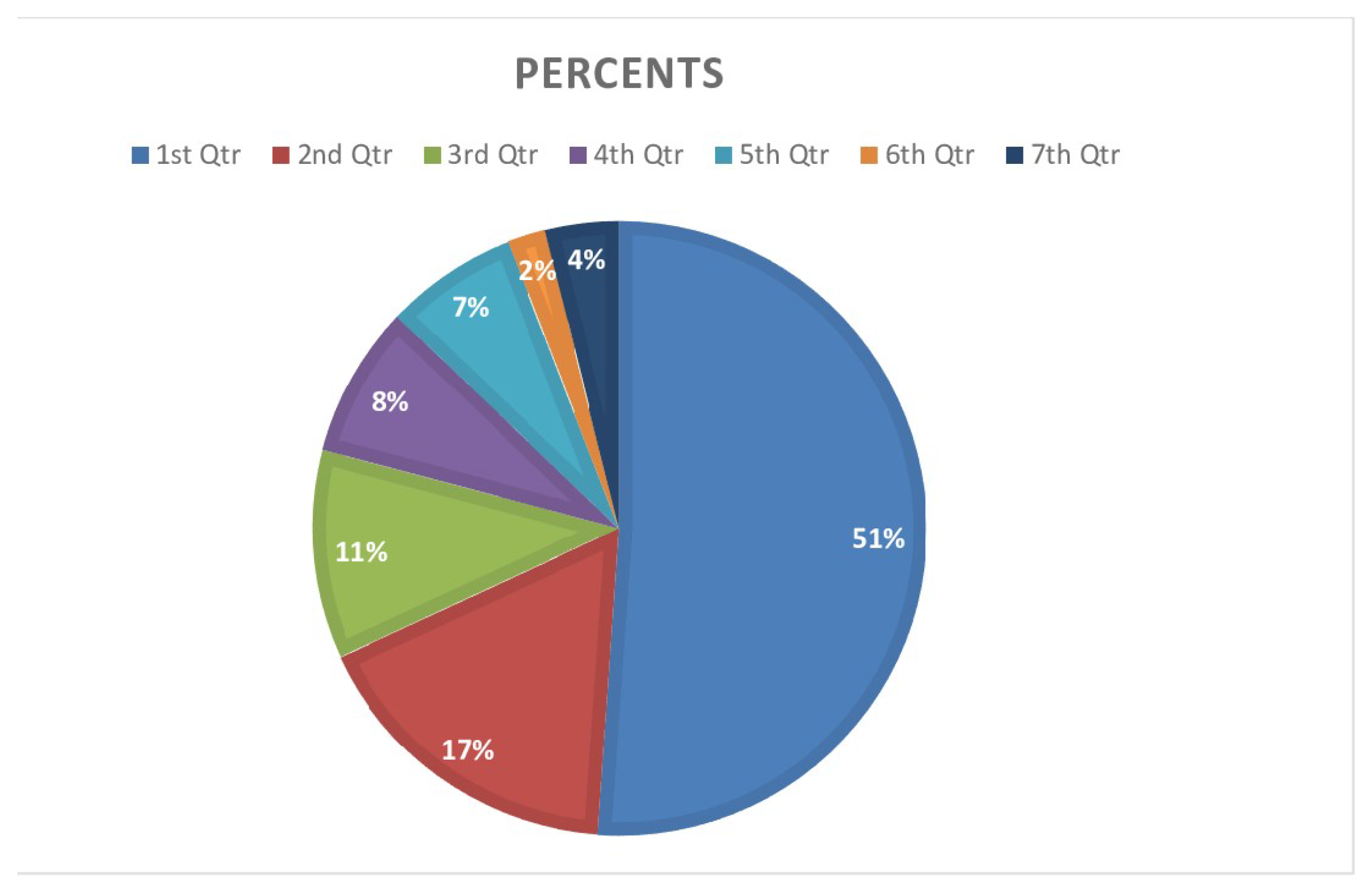
The energy consumption on Metrorex Line 2 is mainly (see
Figure 1 (T,V,L,E,P,I,O), PieChart, percentages) consumed in T = Traction, V = Ventilation, L = Lighting, E = Elevator, P = Pump, I = Installed cabinets, and O = Others, among which the traction energy plays the most important role.
> with(Statistics);
PieChart(W, sector = 0 .. 360, datasetlabels = default);
(the PieChart command generates a pie chart for the specified data in Maple 18 or in excel).
Figure 1.
Energy consumption on Metrorex Line 2.
Figure 1.
Energy consumption on Metrorex Line 2.
The minimal energy consumption of the Bucharest metro in 2021 is given in
Table 1 (
,
,
,
,
,
):
3.4. Viscosity Solutions of the PDE (1)
Hamilton–Jacobi–Bellman PDEs are of central importance in applied mathematics. A major drawback, however, is that the HJB PDE admits classical solutions only for a sufficiently smooth value function, which is not guaranteed in most situations. Several notions of generalized solutions have been developed to cover such situations, for example including viscosity solutions (see [
4]).
Viscosity solutions need not be differentiable anywhere and thus are not sensitive to the classical problem of the crossing of characteristics. The only regularity required for this kind of solution is continuity.
By defining viscosity solutions for the first order PDE
, we denote by
the differential operator attached to PDE
and we attach two PDE inequations
(resp.
).
Let be a bounded, open set.
Definition 1. A continuous function is a viscosity sub-solution (resp. viscosity super-solution) of PDE (1), if for any point and any function φ such that and (resp. ) in a neighborhood of , we have (resp. ), where D is the differential operator attached to PDE (1).
A continuous function is a viscosity solution of if it is both a viscosity sub-solution and a viscosity super-solution.
We define the Euclidean distance to the boundary given by the formula .
Lemma 1. The function distance to the boundary d is uniformly Lipschitz.
Proof. The set
is compact. Consequently, for each
there exists
such that
. Let us have another point
and
. Then
The converse is obvious. Hence,
□
Open problem Using the distance d, can we construct a viscous solution of PDE (1)?
Open problem A posynomial is a function of the form where all the coordinates , and all the coefficients are positive real numbers, and the exponents are real numbers. Posynomials are closed under addition, multiplication, and non-negative scaling.
Using a posynomial, can we build a viscous solution of PDE (1)?
The viscosity solution theory is a mathematical framework used to also study the solutions of linear PDEs. This approach aims to provide a solution in a weaker sense, before establishing its regularity. The theory is useful in situations where the existence of general solutions is difficult to establish, as is often the case with linear equations. By starting with a weaker solution and then showing regularity, this approach provides a systematic way to study and understand linear PDEs.
4. Six Forces Acting on the Moving Train
In the most general situation, the forces acting on the train are: traction force, cruising force, braking force, descendant or ascendant force, and centrifugal force [
2].
Let be the length of a certain interstation. The previous train simplified model can be improved with a complete model adding traction force, cruising force, braking force, descendant or ascendant force, and centrifugal force. For that, we need , and as decision constants given by the metro staff.
Let
be the maximum available traction force according to the motor characteristic; let
be the force to keep cruising at position
x (air friction force); let
be the maximum available braking force; and let
be a binary variable with no unit. All of these determine a resultant force as a piecewise
accolade force with four branches
where
is the speed. The force
must be greater than 0 in traction mode or less than 0 in braking mode. It stands for the output force acting upon the train given by ATO. A positive value of
denotes that the train is motoring.
The value
indicates that the train control mode is
, while the value
stands for the case in which the control mode is
. For example, coasting is implemented when the train arrives at
, and
is thus set as 0. When the train speed increased to the limit,
will be implemented again and
becomes 1. Then, the resistance force
is used to decide the following control regimes. Denote
. The function
can be written as
where
and
are the speed limit and train speed at position
x, respectively. The value
represents the train control mode in the previous distance step, where
represents the length of the distance step. The force
is the resultant resistance, consisting of friction resistance, air drag, and additional resistance caused by grades and curves.
In motion, the mass of the train is
where
is the rolling stock mass;
is the number of passengers on the train in the
n-interstation; and
is the average mass of a person. The actual train mass is necessary for computing the traction force.
By linear interpolation, we obtain a simplified model of traction force,
where
,
, and
represent train masses when the train is empty, nominally loaded, and maximum loaded, respectively;
,
, and
indicate the traction force in the above three circumstances.
We introduce three forces: (1)
with
coefficients fixed by rolling stock manufacturers; (2)
is the resistance caused by the gradient; and (3)
is the resistance caused by the trajectory (the track). The total force
determines the resultant force
acting upon the train.
Let be the mass of the moving body. If the train goes downhill, then the force appears, where g is the gravitational acceleration and is the angle of the slope (negative means downhill).
If the track is curvilinear, then the centrifugal force appears, where v is the velocity of the moving body, is the radius of curvature.
When cruising is applied, the resultant force
should be equal to zero; then,
is the resultant
4.1. Additional Constraints
Train control schemes should be subject at least to the following additional constraints:
(i) For operational safety and passenger comfort, the acceleration should be limited within a proper range, i.e., ;
(ii) The train must stop when it arrives at a station, i.e., for each ;
(iii) Train velocity must be positive and not exceed the speed limit, i.e., .
4.2. Broken Extremals
Let us explain how we can use broken extremals and the Erdmann–Weierstrass corner conditions in order to describe the metro optimal movement.
We accept that the objective functional (mechanical work)
can be written
with corners at
,
, and
, and the ends at left and right being variable in each case.
For each corner
,
,
, we must have two Erdmann–Weierstrass conditions
Therefore, on each interval, we have one Euler–Lagrange equation and two Erdmann–Weierstrass corner conditions.
5. Bucharest Subway Structure
Let us underline the structure of the subway in Bucharest.
The Bucharest Metro (see [
13]) was first considered in 1930 and again in 1952 when the General Directorate of the Metro was established, although it was thought that the subsoil conditions would require an excessive amount of metal to support the tunnels.
The first section of the subway line in Bucharest was built between 1975 and 1979, this underground construction being designed and built with Romanian machinery. The current network of the Bucharest metro was built at a sustained pace until 1989, with the first three main lines being completed.
In 2020, the subway in Bucharest stretched on a route with a length of 77 km of double railway. To date, five main lines of the underground metro have been built, with 63 metro stations, these being spaced, on average, at 1.5 km. Following the subway map (see Internet), highway 1 forms a belt that encircles the city center, having a common segment with the route of highway 3. Highway 2 crosses the city from north to south, and highway 3 crosses the municipality from west to east.
The number of people using the subway in Bucharest varies between 120,000 and 250,000 passengers. Until 1990, Bucharest metro trains were manufactured only in Romania, at the IVA plant in Arad. After 1990, over 40 Bombardier trains were purchased, replacing some of the IVA trains. We mention that the travel speed of the subway trains in Bucharest is 80 km/h, and the commercial speed is 40 km/h.
In this section, case studies on Metrorex Line 2 in peak hours are employed to illustrate the effectiveness of the improved train control and integrated optimization model.
The propulsion system is designed to achieve the traction and braking diagram. Functional data: The propulsion system is designed to achieve a traction and braking diagram with (A = force(kN), B = velocity(km/h)).
The metro lines in operation at Bucharest subway are: M1: Crângași-Dristor-(Pantelimon)-Obor-Piața Victoriei-Gara București Nord-Crângași; M2: Pipera-Piața Unirii-Berceni; M3: Preciziei-Eroilor-Anghel Saligny; M4: Gara de Nord-Străulești; M5: Râul Doamnei-Eroilor.
6. Conclusions
We have developed a mathematical rescheduling model that can tackle the diverse optimization problems in metro energy management. This model classifies different problems based on their objective function, decision variables, and instant power demand evaluation. The objective function is a mechanical part and the problem itself is an optimal control problem, which minimizes the objective function subject to constraints defined by (ODEs). This problem is solved through a Hamilton–Jacobi–Bellman (PDE) of first order. The goal is to reduce the metro’s electricity usage, which in turn results in lower global energy consumption. Six forces affect the movement of the trains, which are outlined in
Section 4 and used to form the system of ODEs. To solve the problem, we propose to find viscosity solutions of HJB PDEs. Optimizing the energy-efficient train control and service timetable can significantly reduce energy consumption in existing urban rail systems, with low capital investment and minimal changes to operating rules. The conducted research has also been applied in real-world problems, covering the design, execution, and exploitation stages.
This paper focuses on reducing the energy consumption of metro trains in existing urban rail systems through the use of energy-efficient train control and optimization of service schedules.
Energy-efficient train control and service timetable optimization are preferred to reduce metro train energy consumption in existing urban rail systems. Energy saving could be achieved with relatively low capital investment and minor modifications of the operating rules, via optimal control results.
The bibliography [
1,
2,
3,
4,
5,
6,
7,
8,
9,
10,
11,
12,
13,
14] also describes the stages of practical application of the conducted research, being the problems of design, execution and exploitation.


