Abstract
A new and simple blockwise empirical likelihood moment-based procedure to test if a stationary autoregressive process is Gaussian has been proposed. The proposed test utilizes the skewness and kurtosis moment constraints to develop the test statistic. The test nonparametrically accommodates the dependence in the time series data whilst exhibiting some useful properties of empirical likelihood, such as the Wilks theorem with the test statistic having a chi-square limiting distribution. A Monte Carlo simulation study shows that our proposed test has good control of type I error. The finite sample performance of the proposed test is evaluated and compared to some selected competitor tests for different sample sizes and a variety of alternative applied distributions by means of a Monte Carlo study. The results reveal that our proposed test is on average superior under the log-normal and chi-square alternatives for small to large sample sizes. Some real data studies further revealed the applicability and robustness of our proposed test in practice.
MSC:
62G10; 60G10; 60G15; 62E10
1. Introduction
In time series analysis, testing whether a time series process follows a Gaussian distribution is customarily conducted as preliminary inference on the data before further analysis can be performed. This makes the development and use of normality tests for time series data a vital area in the field of applied and theoretical statistics. Various tests for assessing consistency to Gaussianity in time series processes have been developed and widely reported in literature (see [1,2,3,4,5], among others). These tests make use of various forms of mathematical characterization of the underlying time series process in developing the test statistics. For example, Epps [1] proposed a test based on the analysis of the empirical characteristic function. Lobato and Velasco [2] as well as Bai and Ng [3] developed tests based on the skewness and kurtosis coefficients. Moulines and Choukri [6] based their test on both the empirical characteristic function as well as the skewness and kurtosis coefficients. Bontemps and Meddahi [7] used moment conditions implied by Stein’s characterization of the Gaussian distribution. Psaradakis and Vavra [5] proposed a test by approximating the empirical distribution function of the Anderson Darling’s statistic, using a sieve bootstrap approximation. On the other hand, Rao and Gabr [8] proposed their test based on the bispectral density function.
As alluded to by Lobato and Velasco [2] as well as Bai and Ng [3], in time series analysis, testing for normality is customarily performed by utilizing the skewness and kurtosis tests. This is because of their lower computational cost, popularity, simplicity and flexibility. The moment-based tests by Lobato and Velasco [2], as well as Bai and Ng [3], used classical measures of skewness and kurtosis involving standardized third and fourth central moments. To handle the issues of data dependence, Lobato and Velasco [2] used the skewness–kurtosis test statistic, but studentized by standard error estimators that are consistent under serial dependence of the observations. On the other hand, to cater for dependence, Bai and Ng [3] used the limiting distributions for the third and fourth moments when the data are weakly dependent. One possible way to alleviate the dependence problem in moment-based tests is to employ techniques that can address the correlation that exists between the time series observations. Such techniques may include some bootstrapping and resampling procedures. The blockwise-empirical likelihood (BEL) technique is one such procedure that is widely used to address issues of correlated data in time series processes (see [9]).
The use of the empirical likelihood (EL) methodology (see [10,11] for more details) to develop simple, powerful and efficient moment-based tests for normality has received enormous attention (see [12,13,14,15] for more insight). The application of the EL methodology on independent and identically distributed (i.i.d.) data has been studied in a variety of contexts, including inference on the skewness and kurtosis coefficients (see [16] for more details), but our interest in this study concerns the application of the EL methodology on weakly dependent time series processes. Due to the underlying dependence structure in time series processes, the formulation of the EL usually fails, and in order to apply the EL methodology to time series data, serial dependence among observations needs not to be ignored. As a remedy, Kitamura [9] proposed the BEL methodology for weakly dependent processes. This proposed technique has been shown to provide valid inference in various scenarios with time series processes in a wide range of problems (for example, see [17,18,19,20,21,22,23,24,25,26,27], among others). Similarly to the i.i.d. EL version, the BEL method creates an EL log-ratio statistic with a chi-square limit for inference. However, the BEL construction crucially involves blocks of consecutive observations in time, which serves to capture the underlying time-dependence structure. It is important to note that the choice of block sizes is vital, as it determines the coverage performance of the standard BEL methodology [9]. Thus, the performance of the BEL is largely dependent on the choice of the block size b, which is an integer defined on .
In this article, we propose a goodness of fit (GoF) test statistic for Gaussianity in weakly dependent stationary autoregressive processes of order one (AR(1)). We focused on AR(1) processes because they are commonly encountered in the field of econometrics as well as applied and theoretical statistics. The GoF test is constructed based on the third and fourth moments, employing the standard BEL methodology. Thus, our proposed procedure applies the standard BEL methodology that non-parametrically accommodates the dependency in the time series process whilst exhibiting some useful properties of EL, such as Wilks’s theorem. The next section will present the development of the proposed test statistic. The article will further present the finite sample performance of our proposed test in comparison with other existing competitor tests. Some real data applications will be conducted and presented. Lastly, conclusions and recommendations will be drawn based on the findings of the Monte Carlo (MC) simulations as well as the real data studies.
2. The Blockwise Empirical Likelihood Ratio Test Statistic
Let be a sample of n consecutive equally spaced observations from a strictly stationary, real-valued, discrete-time stochastic process taking values in . Since this is a general definition, for this study we considered for an autoregressive process of order 1 model that is assumed to be stationary. Thus, we define the autoregressive process of order 1 as given by
where is a constant such that . According to Nelson [28], Wei [29], as well as Box et al. [30], among others, the requirement is called the stationarity condition for the AR(1) process. The problem of interest is to test the composite null hypothesis that the one-dimensional marginal distribution of is Gaussian, that is
Based on the observed sample ’s, we are interested in the alternative hypothesis that the distribution of is non-Gaussian. Without loss of generality, we then proposed to use standardized random variables of the sample observations. To achieve this, we adopted the common transformation technique of standardizing observed data points to by subtracting the mean and dividing by . Thus, from the initial hypothesized framework in (1), we estimate and by their maximum likelihood estimators, i.e., and . Let , . Then, the composite null hypothesis becomes
The parameter is unknown. Bai and Ng [3] derived and proved the limiting distribution of the sample skewness and kurtosis for a stationary time series process under arbitrary and before extending the general results to (or, equivalently, ) and (or, equivalently, ) under normality. Following the empirical likelihood methodology, the moment of the transformed data, , , has sample moments of the form , where . The probabilities ’s are components of the empirical likelihood, , which is used to maximize the empirical likelihood function given empirical constraints. Under the null hypothesis that the standardized observations are from a Gaussian distribution, the unbiased empirical moment equations are
where the probability parameters ’s fulfill the two fundamental properties of probability theory which states that and . We now consider for the problem of inference about the process mean . Considering the unbiased empirical moment equations in (2), the hypotheses for the ELR test can be written as
where r takes values 3 and 4. Since there is dependence in the time series data, one cannot use the traditional EL by Owen [11], which was specifically developed for independent, identically distributed data. Thus, the i.i.d. formulation of EL fails for dependent data by ignoring the underlying dependence structure. Therefore, following the works of Kitamura [9], we then adopted the standard BEL (also discussed by Nordman et al. [26], and Kim et al. [31], among others) to construct the test statistic. The technique involves choosing an integer block length and forming a collection of length b data blocks, which could possibly be maximally overlapping (OL) as given by
or non-overlapping (NOL) as given by
In both cases, all blocks have constant length b for a given sample size n. For inference on the mean parameter , each block in the OL collection , contributes a centered block sum given by
or with NOL blocks
The blocking schemes (4) and (5) aim to preserve the underlying dependence between neighboring time observations. We then consider the profile blockwise empirical likelihood function for given as
where . Under a zero-expectation constant, assesses the plausibility of through utilizing probabilities , which are assigned to the centered block sums to maximize the multinomial likelihood, . In the absence of the mean constraint in (6), the maximization of the multinomial likelihood is performed when each , which leads to the corresponding BEL ratio
The computation of for the BEL version is similar to that described by Owen (1988, 1990) for i.i.d. data. Thus, when lies within the interior convex hull of , then for the standard Lagrange multiplier arguments imply that the maximum is attained at probabilities
with the Lagrange multiplier satisfying
For more computational details of this result, see Kitamura [9]. Further, Kitamura [9] alluded that, under certain mixing and moment conditions, as well as for traditional small b asymptotics, that is, , the log-EL ratio of the standard BEL has a chi-square limiting distribution. Thus, under regularity conditions that can be found in [9], one can easily show that
at the true mean parameter (for detailed proof, see [9]). Nordman et al. [26] as well as Kim et al. [31] further provided a detailed rationale and explanation to support (7), that is, the limiting distribution for the log-EL ratio of weakly dependent data has a chi-square limiting distribution. For this log-EL ratio, represents an explicit block adjustment factor in (7) to ensure the distributional limit for the log-EL ratio of the BEL. A block length of results in the EL distributional result of Owen [10,11]. Our choice of the ideal block length for the proposed test statistic is discussed in the next section. Now, let us consider the −2 log-likelihood ratio test statistic for the null hypothesis, which is given by
In order to determine whether to reject or not reject , we used the likelihood ratio to compare to size-adjusted critical values. Thus, for our proposed blockwise empirical likelihood ratio test, we propose to reject the null hypothesis if
where is the critical value and , with . The values of G are integers representing the third and fourth moment constraints that are used to maximize the test statistic. Our proposed test statistic (9) is a cumulative sum (CUSUM)-type test statistic and it is well accepted in the change point literature (for example, see [32,33,34,35]). Alternatively, one can consider the test statistic based on the Shiryayev-Roberts (SR) approach (for example, see [36]). However, for empirical likelihood moment-based GoF tests, it has been demonstrated that the CUSUM-type test statistic is superior in power performance as compared to the SR-type test statistic [12,13,15].
The classical EL method can be considered a special case of the BEL method (without data blocking, thus, ). That is when implies both for OL blocks and for NOL blocks reduces to n. Since the standard BEL method mimics the i.i.d. case, under the condition that one can show that (8) for (3) has a chi-square limiting distribution. Applying the EL methodology and the Wilks theorem [37], Shan et al. [12] showed that, under the usual classical case of the EL (with standardized data), a similar test statistic, , for , with has a chi-square limiting distribution (for further details, see lemma 2.1 and proposition 2.1 and their respective proofs by Shan et al. [12]). Referring to the proofs by Owen [10,11], Nordman et al. [20] reported that the EL with i.i.d. has a key feature in allowing a nonparametric casting of the Wilks theorem, meaning, when evaluated at the true mean, the log-likelihood ratio has a chi-square limiting distribution. This was first extended to the BEL method with weakly dependent processes by Kitamura [9], who showed that a similar result for the classical EL method applies to the BEL method. However, according to [9], the BEL method requires choosing a suitable block size b for the optimal coverage accuracy. The next section will present a MC simulation-based approach to determine the ideal block size for the proposed test statistic.
3. Monte Carlo Simulation Procedures
3.1. Block Size Selection
The standard implementation of the BEL method typically involves data blocks of constant length for an observed time series and therefore requires a corresponding block length selection. In addition, the performance of the BEL method often depends critically on the choice of the block length. In the literature, little is known about the best block size selection for optimal coverage accuracy with the standard BEL method. In practice, researchers usually borrow from the block bootstrap literature, where optimal orders for block sizes vary in powers of the sample size such as or (see [38,39], among others). Additionally, data-driven block length choices also borrow from bandwidth selection with kernel spectral density estimators such as the Bartlett kernel (see [9,40]) where such block selections are also based on a fixed block size order (i.e., ). Kitamura [9] recommended that the empirical block selections for the BEL method should involve estimated adjustments to the block order , and this may not in fact be optimal for the coverage accuracy of the standard BEL method. In implementation, the block order is usually adjusted by a constant factor, which is often set to C = 1 or 2 [31,39]. Several studies that looked at weakly dependent time series data (both autoregressive and moving average models) have adopted the use of the optimal block order of (see [31,40], among others).
Using R, we conducted an extensive MC experiment to establish the ideal block sizes to use for an AR(1) process, which is our time series process of interest. To achieve this objective, we assessed the coverage accuracy of the BEL method on inference about the mean parameter , mean for a stationary, weakly dependent time series) at the 0.05 nominal level for different sample sizes (n = 100, 250, 500 and 1000) with varying choices of block sizes. As investigated and alluded to by Nordman et al. [26], the coverage accuracy of the BEL method depends on the block length b. We borrowed the works of Kim et al. [31] on the choice of block order adjustment, and constant factor C, which was set to C = 0.5, 1, 2 and 3. In essence, we employed four different block sizes of the form , where C = 0.5, 1, 2, 3. Thus, we considered varying the block sizes in powers of the sample sizes by utilizing . Under the null hypothesis, we generate data from the following AR(1) process.
where is i.i.d. , and the autoregressive parameter takes nineteen values from −0.9 through to 0.9 at 0.1 intervals apart. We reported the results for both the detailed grids of negative and positive values of because our test statistic is proposed for applications on . Coverage probabilities for both the BEL method with OL and NOL blocks were assessed. However, it is important to note that NOL blocks are known to perform either similarly or slightly worse than the OL block versions [31]. We only opted for the normal distribution of the error term since the EL method has been reported to have small coverage errors in time series data for both normal and non-normal errors [41,42]. In order to assess the overall performance of the BEL method under the several simulated scenarios, the mean, as well as the mean average deviations, were used.
From the results (see Table 1 and Table 2), we can see that under small sample sizes (i.e., n = 100 and 250) the standard BEL method performs well with OL blocks and block sizes of and . Under these sample sizes, the BEL method with NOL blocks performed slightly less than the BEL method with OL blocks. In addition, from Table 2, the coverage probabilities based on the BEL method with block sizes of continue to be the less accurate statistic. The performance of the BEL method with block sizes , and is comparable for moderate to large sample sizes (i.e., n = 500 and 1000). It is important to note that when , the BEL method is generally conservative, and when , the BEL method is regarded as largely permissive or anti-conservative. This poor coverage performance was also reported in MC simulations conducted by Nordman et al. [26]. This is a major weakness of the standard BEL method as is it sensitive to the strength of the underlying time-dependence structure (see [20,26,31]). However, due to the simplicity, flexibility, and wide range of applications of the standard BEL method in various applied and theoretical statistics problems, we adopted it for our proposed test statistic. From the simulation results, we decided to adopt block sizes and for further investigation because of the better coverage accuracy for the BEL method for both the NOL and OL blocks.

Table 1.
Coverage probabilities for 95% BEL CIs for the mean of ( i.i.d. standard normal), with for NOL and OL blocks of size using 5000 simulations. Means and mean average deviations (from 0.95) of coverage probabilities are indicated in bold.
Table 2.
Coverage probabilities for 95% BEL CIs for the mean of ( i.i.d. standard normal), with for NOL and OL blocks of size using 5000 simulations. Means and mean average deviations (from 0.95) of coverage probabilities are indicated in bold.
3.2. Finite Sample Performance
This section compares the finite sample behavior of the proposed testing procedure in different situations. The R statistical package was used for all MC simulations. In order to conduct the MC power study, firstly we had to compute the and size-adjusted critical values of the proposed test. The rationale behind having dependent critical values is that in addition to sample size, the type I error control for weakly dependent time series process is heavily dependent on (for example, see [43]). We simulated an AR(1) model with normal errors. Without a loss of generality, we generated 20,000 samples of size 100, 500 and 1000 with taking values and . These simulations were conducted for both the BEL with NOL and OL blocks for block sizes and . The upper alpha quantile of the empirical distribution of the test statistic was considered the critical value for each simulated scenario. These critical values are correct only if the AR(1) model is the data-generating process and the errors are indeed normal (for example, see [44]).
Under the null hypothesis, we generate data from an AR(1) process defined in (10), where the autoregressive parameter (similar to [2,4]). We report the findings for a detailed grid of positive values of because positive autocorrelation is particularly relevant for many empirical applications. The error terms are i.i.d. random variables, which may follow any of the following seven alternative distributions:
- Standard normal ,
- Standard log-normal (Log N),
- Student t with 10 degrees of freedom ,
- Chi-squared with 1 and 10 degrees of freedom ,
- Beta with parameters (2, 1) ,
- Uniform on [0, 1] .
To simulate the process defined in (10), we generated independent realizations for these distributions. When , the process in (10) is not stationary. To cater to this challenge, we adopted the approach used by Nieto-Reyes et al. [4] of disposing some observations. We set our to 1000 and n = number of replications—. These alternative distributions have been used before for similar purposes (see [2,4]). Before the main power study, we conducted a MC experiment to further establish the block size (i.e., or ) and the BEL block structure (i.e., NOL or OL) that will result in the optimal power for our proposed test. In Table 3, we report the empirical rejection probabilities for the proposed tests with NOL and OL blocks for block sizes and . We considered three sample sizes, n = 100, 500 and 1000, with . Four alternative distributions (i.e., Log N, , and ) for the error term were used. In these experiments, 5000 replications were carried out at a nominal level of . The main conclusion derived from these experiments is that the BEL statistic with both the NOL and OL blocks and a block size of were generally superior under almost all the simulated cases. The proposed procedure for the NOL and OL blocks gave comparable power. Due to the latter, we decided to adopt OL blocks with block sizes . Our choice of block sizes was also recommended and used by Kitamura [9] and also, as stated earlier, NOL blocks are known to perform either similarly or slightly worse than the OL block versions [31].
Table 3.
Empirical rejection probabilities of the process defined in (10) for NOL and OL blocks with varying block sizes at the 0.05 nominal level for using 5000 replications.
For the main power comparison study, we considered some well-known existing procedures to test if a stationary process is Gaussian. We adopted 3 (three) competitor tests, namely the Epps and Pulley (EPPS) test (see [1] for more details), the Lobato and Velasco (LV) test (see [2] for further insight) and the Psaradakis and Vavra (PV) test (see [5] for further insight). These tests have been considered in other studies where power comparisons have been conducted, and these include studies by Lobato and Velasco [2] as well as Nieto-Reyes et al. [4]. Our choice of competitor tests was also limited to the availability of the tests in R as well as tests that reasonably control type I error. The results of the MC power study are presented in Table 4, Table 5 and Table 6. We report the empirical rejection probabilities for the proposed blockwise empirical likelihood ratio test, with OL blocks of size (referred to as BELT henceforth). As in the previous MC simulation experiment, we considered three sample sizes, n = 100, 500 and 1000, with . Seven alternative distributions for the error term were used (i.e., , Log N, , , , and as defined earlier). Each simulation scenario was repeated 5000 times at a nominal level of .
Table 4.
Empirical rejection probabilities of the process defined in (10) at the 0.05 nominal level for using 5000 replications.
Table 5.
Empirical rejection probabilities of the process defined in (10) at the 0.05 nominal level for using 5000 replications.
Table 6.
Empirical rejection probabilities of the process defined in (10) at the 0.05 nominal level for using 5000 replications.
The findings in Table 4, Table 5 and Table 6 shows that our proposed test, the BELT, has good control of type I error as compared to all other tests considered. For small samples (i.e., ), the BELT test was superior under the alternative distribution (see Table 4). The BELT and PV tests were on average the most powerful under the Log N alternative distribution. The BELT test was superior under the , whilst the EPPS test was superior under the and alternative distributions. The LV test was overly the most powerful test under the distribution. Our proposed test was on average the second most superior test under the and distributions.
For medium sample sizes of (see Table 5), our proposed test overly outperformed all tests under Log N, , and alternatives. However, under the Log N distribution, our proposed test is comparable to the LV test. On the other hand, the LV test was generally superior to all other tests under the alternative distribution. Our proposed test was generally the second most powerful test under the alternative distribution. The EPPS and PV tests are on average the least powerful tests.
For large samples ( in Table 6), the BELT and LV tests are the most superior under the Log N alternative distribution. When the alternative was , the LV test was on average the most powerful test. Our proposed test, the BELT, was the most superior test under the , and alternative distributions. The EPPS test was on average the most powerful under the distribution, with the BELT test being the second most powerful test.
In order to obtain a clearer visualization of the performance of the different tests, the ranking procedure was used (for example, see [15]). Table 7 shows the ranking of all the tests considered in this study according to the average powers computed from the values in Table 4, Table 5 and Table 6. The rank of power is based on the respective alternative distributions and sample sizes. Using average powers, we can select the tests that are, on average, most powerful against the respective alternative distributions. One of the major findings derived from the ranking is that on average our proposed test was superior under the Log N, and for small to large samples.
Lastly, we decided to determine the computational cost of the new algorithm by focusing on the computational time of the proposed test as compared to that of the competitor tests. For accessing and comparing the computational times, we opted for the R benchmark. These experiments were conducted using a notebook installed with 64 Bit Windows 10 Home edition. The processor was a 4th generation Intel Core i5-4210U, which has a speed of 1.7 GHz cache and random access memory of 4GB PC3 DDR3L SDRAM. The sample size was set to 100 with 1000 replications for each test where under a chi-square alternative distribution with 1 degree of freedom. The results (see Table 8) show a clear advantage of our proposed approach to that of the PV test.
Table 8.
Comparisons of computational times (in seconds) for the studied tests.
4. Real Data Applications
4.1. The Canadian Lynx Data
Firstly, we used the Canadian lynx dataset, which has been extensively used in various statistical applications and previously found to be non-Gaussian [1,4,8]. The dataset has been shown to model well with an autoregressive time series process (see [45,46,47], among others). The Canadian lynx dataset consists of 114 observations of the annual record of the number of lynxes trapped in the Mackenzie River district of North-West Canada for the period from 1821 to 1934 (see [45] for more details). The Canadian lynx data are
269, 321, 585, 871, 1475, 2821, 3928, 5943, 4950, 2577, 523, 98, 184, 279, 409, 2285, 2685, 3409, 1824, 409, 151, 45, 68, 213, 546, 1033, 2129, 2536, 957, 361, 377, 225, 360, 731, 1638, 2725, 2871, 2119, 684, 299, 236, 245, 552, 1623, 3311, 6721, 4254, 687, 255, 473, 358, 784, 1594, 1676, 2251, 1426, 756, 299, 201, 229, 469, 736, 2042, 2811, 4431, 2511, 389, 73, 39, 49, 59, 188, 377, 1292, 4031, 3495, 587, 105, 153, 387, 758, 1307, 3465, 6991, 6313, 3794, 1836, 345, 382, 808, 1388, 2713, 3800, 3091, 2985, 3790, 674, 81, 80, 108, 229, 399, 1132, 2432, 3574, 2935, 1537, 529, 485, 662, 1000, 1590, 2657, 3396.
The goal of this section was to carry out a bootstrap study to assess the robustness and applicability of our proposed test in practice. The approach was to use a sample of size 100 by randomly selecting from the Canadian lynx data and then test for normality at 0.05 level of significance. Before the bootstrap study, we conducted the augmented Dickey–Fuller test for stationary assumption on the complete dataset. The augmented Dickey–Fuller Test (Dickey–Fuller = −6.31, p-value = 0.01) revealed that the Canadian lynx data are stationary. We then used a graphical approach to access the normality and the findings (see Figure 1) support the findings reported by Rao and Gabr [8], Epps [1] as well as Nieto-Reyes et al. [4] that the data are indeed non-normal. Having confirmed that the data are stationary and non-Gaussian, we then employed a bootstrap technique using the proposed test where we randomly removed 14 observations of the Canadian lynx data and then derived the p-value from the remaining observations. We also repeated this technique 5000 times for the EPPS and LV tests. We considered these tests because they performed quite well in our MC power study. The findings showed that the proposed BELT test had a p-value of . The p-values that were obtained for the other tests, that is, for the EPPS test and for the LV test, were all suggestive for one to conclude that the Canadian lynx data are indeed non-Gaussian. The p-values obtained from the traditional tests as well as our proposed test proved to be consistent in illustrating the non-normality of the Canadian lynx data. Thus, our proposed test statistic has demonstrated robustness and that it is applicable when applied to some non-Gaussian real-life data.
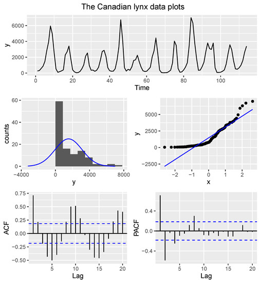
Figure 1.
Diagnostic plots for the Canadian lynx data. The upper plot shows a time-series plot, which reveals evidence of stationarity. The middle plots are the histogram (middle-left) and the quantile–quantile plot (middle-right), and both plots suggest that the time series process has a non-normal distribution. The lower plots show the autocorrelation functions, and for both plots, the autocorrelations are close to zero, giving further evidence of stationarity.
4.2. The Souvenir Data
This real data study intends to demonstrate the practical applicability of our proposed test under a normally distributed time series process using 84 monthly sales for a souvenir shop at a beach resort town in Queensland, Australia (see [48] for more details). These sales were recorded from January 1987 to December 1993 and have been used for various time series applications (for example, see [49,50], among others). However, the time series data are not consistent with the normal distribution and are not stationary [49]. To verify these claims, we conducted tests for the Gaussianity and stationarity of a time series process using the k random projections test and the augmented Dickey–Fuller test, respectively. We supplemented these tests with diagnostic plots for assessing the stationarity and normality in time series processes (see Figure 2).
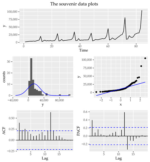
Figure 2.
Diagnostic plots for the souvenir data. The upper plot shows a time-series plot, which reveals evidence of non-stationarity. The middle plots are the histogram (middle-left) and the quantile–quantile plot (middle-right), and both plots suggest that the time series process has a non-normal distribution. The lower plots show the autocorrelation functions.
The results revealed that the monthly sales for the souvenir shop do not follow a Gaussian process (k = 16, p-value < ) and are not stationary (Dickey–Fuller = −2.0809, p-value = 0.5427), which is a similar finding reported by the graphical plots presented in Figure 2. Since the goal is to examine the performance of our proposed test under a normally distributed time series process, we used the Holt–Winters exponential smoothing to obtain the forecast errors for the monthly sales of the souvenir shop, which are well-known to be stationary and consistent with normality [49]. The Holt–Winters exponential smoothing was ideal because the time series process of the log of monthly sales for the souvenir shop can be described using an additive model with a trend and seasonality. Thus, to obtain the forecasts, we fitted a predictive model for the log of the monthly sales. We then obtained the forecast errors and used the same testing procedures reported earlier to assess whether these errors are indeed normally distributed and stationary.
From the plots (see Figure 3), it is clear that the forecast errors are normally distributed and stationary. The k random projections test (k = 16, p-value = 0.7923) and the augmented Dickey–Fuller test (Dickey–Fuller = −4.5942, p-value = 0.01) also revealed that the forecast errors follow a Gaussian process and are stationary. To demonstrate the robustness and applicability of our proposed test, we conducted a bootstrap study (using 5000 replications) by randomly deleting two observations at a time in order to test whether the forecast errors follow a Gaussian process. For the sake of comparison, this procedure was repeated for each of the selected competitor tests. The respective p-values were noted under the null hypothesis that the forecast errors follow a Gaussian process. At level of significance, our proposed test reported a p-value of 0.6418158, whilst the EPPS, LV and PV tests reported p-values of 0.3776963, 0.7008432 and 0.611926, respectively. Thus, our proposed test as well as the selected competitor tests suggest that the forecast errors of the monthly sales for the souvenir shop follow a Gaussian process. This is consistent with the graphical plots presented in Figure 3 as well as past applications [49]. This real data study has further demonstrated the robustness and applicability of our proposed test in practice.
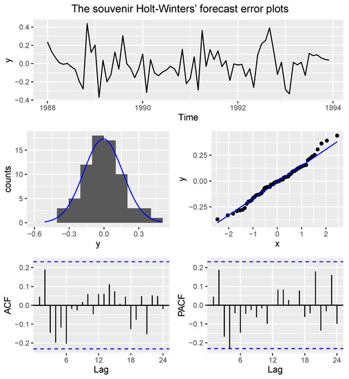
Figure 3.
Diagnostic plots for the souvenir forecast errors. The upper plot shows a time-series plot, which reveals evidence of stationarity. The middle plots are the histogram (middle-left) and the quantile–quantile plot (middle-right), both plots suggest that the time series process has a normal distribution. The lower plots show the autocorrelation functions, and for both plots, the autocorrelations are close to zero, giving further evidence of stationarity.
5. Conclusions
A simple BEL-based procedure to test if a stationary autoregressive time process is Gaussian has been proposed. Coefficients of skewness and kurtosis provide convenient measures for characterizing the shape of the normal distribution in time series processes [2,3]. Our proposed test utilizes these moment constraints (i.e., the skewness and kurtosis coefficients) to develop the test statistic. The test applies the standard BEL methodology (see [9] for more details) that nonparametrically handles the dependence in the time series data. The test statistic has a chi-square limiting distribution and has good control of type I error as compared to the existing traditional competitor tests studied. Monte Carlo simulations have shown that our proposed test is overly powerful under the Log N, , and for small to large sample sizes. Further, the real data studies have demonstrated the applicability of the proposed testing procedure in practice. This study has once again proved the efficiency and power of the nonparametric empirical likelihood methodology in developing moment-based GoF tests, and presently this has only been well-established for i.i.d. data [12,13,14,15]. We utilized a CUSUM-type statistic to construct our test statistic, and we advocate for future studies to consider the common alternative to the CUSUM-type statistic, which is to utilize the Shiryayev–Roberts statistic [36].
Through MC simulation experiments, we have also discovered that the coverage performance of the standard BEL method depends on the strength of the underlying dependence structure of the time series process. However, the coverage performance improves with the increasing sample size, and a similar finding was also reported by Nordman et al. [20]. The selection of an optimal block size for the standard BEL method is problematic and is a major drawback of this technique. As a remedy, in the recent past, a few studies have proposed various methods to address this drawback (see [20,26,31]). Nordman et al. [20] proposed a modified BEL method for handling both the short- and long-range dependence for time processes. On the other hand, in order to handle dependence in weakly dependent time processes, Nordman et al. [26] as well as Kim et al. [31] proposed the expansive BEL (EBEL) method and the progressive BEL (PBEL) method, respectively. Unlike the standard BEL method, which depends critically on the choice of block length selection, the EBEL uses a simple and nonstandard data-blocking technique that considers every possible block length. The PBEL requires no block length selection, but rather it uses a data-blocking technique where block lengths increase by an arithmetic progression. All these proposed methods exhibit better coverage accuracy than the standard BEL method, and we suggest that future research can adopt these data-blocking methods for our proposed testing procedure.
Author Contributions
Conceptualization, C.S.M., Y.Q. and R.T.C.; Methodology, C.S.M.; Software, C.S.M.; Validation, C.S.M., Y.Q. and R.T.C.; Formal analysis, C.S.M.; Investigation, C.S.M.; Resources, C.S.M.; Data curation, C.S.M.; Writing—original draft, C.S.M.; Writing—review & editing, C.S.M. and J.M.B. All authors have read and agreed to the published version of the manuscript.
Funding
This study was funded through a research seed grant that was awarded to the main author by the Govan Mbeki Research and Development Centre, University of Fort Hare.
Data Availability Statement
The data presented in this study are available in the respective cited articles/sources.
Acknowledgments
We warmly thank both the associate editor and the anonymous reviewers for their constructive comments and suggestions that have allowed us to improve the paper.
Conflicts of Interest
The authors declare no conflict of interest.
References
- Epps, T.W. Testing that a stationary time series is Gaussian. Ann. Stat. 1987, 1683–1698. [Google Scholar] [CrossRef]
- Lobato, I.N.; Velasco, C. A simple test of normality for time series. Econom. Theory 2004, 20, 671–689. [Google Scholar] [CrossRef]
- Bai, J.; Ng, S. Tests for skewness, kurtosis, and normality for time series data. J. Bus. Econ. Stat. 2005, 23, 49–60. [Google Scholar] [CrossRef]
- Nieto-Reyes, A.; Cuesta-Albertos, J.A.; Gamboa, F. A random-projection based test of Gaussianity for stationary processes. Comput. Stat. Data Anal. 2014, 75, 124–141. [Google Scholar] [CrossRef]
- Psaradakis, Z.; Vávra, M. A distance test of normality for a wide class of stationary processes. Econom. Stat. 2017, 2, 50–60. [Google Scholar] [CrossRef]
- Moulines, E.; Choukri, K. Time-domain procedures for testing that a stationary time-series is Gaussian. IEEE Trans. Signal Process. 1996, 44, 2010–2025. [Google Scholar] [CrossRef]
- Bontemps, C.; Meddahi, N. Testing normality: A GMM approach. J. Econom. 2005, 124, 149–186. [Google Scholar] [CrossRef]
- Rao, T.S.; Gabr, M.M. A test for linearity of stationary time series. J. Time Ser. Anal. 1980, 1, 145–158. [Google Scholar] [CrossRef]
- Kitamura, Y. Empirical likelihood methods with weakly dependent processes. Ann. Stat. 1997, 25, 2084–2102. [Google Scholar] [CrossRef]
- Owen, A.B. Empirical likelihood ratio confidence intervals for a single functional. Biometrika 1988, 75, 237–249. [Google Scholar] [CrossRef]
- Owen, A. Empirical likelihood ratio confidence regions. Ann. Stat. 1990, 18, 90–120. [Google Scholar] [CrossRef]
- Shan, G.; Vexler, A.; Wilding, G.E.; Hutson, A.D. Simple and exact empirical likelihood ratio tests for normality based on moment relations. Commun. Stat. Comput. 2010, 40, 129–146. [Google Scholar] [CrossRef]
- Marange, C.S.; Qin, Y. A simple empirical likelihood ratio test for normality based on the moment constraints of a half-Normal distribution. J. Probab. Stat. 2018, 2018, 8094146. [Google Scholar] [CrossRef]
- Marange, C.S.; Qin, Y. A new empirical likelihood ratio goodness of fit test for normality based on moment constraints. Commun. Stat. Simul. Comput. 2019, 50, 1561–1575. [Google Scholar] [CrossRef]
- Marange, C.S.; Qin, Y. An Empirical Likelihood Ratio-Based Omnibus Test for Normality with an Adjustment for Symmetric Alternatives. J. Probab. Stat. 2021, 2021, 6661985. [Google Scholar] [CrossRef]
- Zhao, Y.; Moss, A.; Yang, H.; Zhang, Y. Jackknife empirical likelihood for the skewness and kurtosis. Stat. Its Interface 2018, 11, 709–719. [Google Scholar] [CrossRef]
- Lin, L.; Zhang, R. Blockwise empirical Euclidean likelihood for weakly dependent processes. Stat. Probab. Lett. 2001, 53, 143–152. [Google Scholar] [CrossRef]
- Bravo, F. Blockwise empirical entropy tests for time series regressions. J. Time Ser. Anal. 2005, 26, 185–210. [Google Scholar] [CrossRef]
- Bravo, F. Blockwise generalized empirical likelihood inference for non-linear dynamic moment conditions models. Econom. J. 2009, 12, 208–231. [Google Scholar] [CrossRef]
- Nordman, D.J.; Sibbertsen, P.; Lahiri, S.N. Empirical likelihood confidence intervals for the mean of a long-range dependent process. J. Time Ser. Anal. 2007, 28, 576–599. [Google Scholar] [CrossRef]
- Nordman, D.J. Tapered empirical likelihood for time series data in time and frequency domains. Biometrika 2009, 96, 119–132. [Google Scholar] [CrossRef]
- Chen, S.X.; Wong, C.M. Smoothed block empirical likelihood for quantiles of weakly dependent processes. Stat. Sin. 2009, 71–81. [Google Scholar]
- Chen, Y.Y.; Zhang, L.X. Empirical Euclidean likelihood for general estimating equations under association dependence. Appl. Math. J. Chin. Univ. 2010, 25, 437–446. [Google Scholar] [CrossRef]
- Wu, R.; Cao, J. Blockwise empirical likelihood for time series of counts. J. Multivar. Anal. 2011, 102, 661–673. [Google Scholar] [CrossRef]
- Lei, Q.; Qin, Y. Empirical likelihood for quantiles under negatively associated samples. J. Stat. Plan. Inference 2011, 141, 1325–1332. [Google Scholar] [CrossRef]
- Nordman, D.J.; Bunzel, H.; Lahiri, S.N. A nonstandard empirical likelihood for time series. Ann. Stat. 2013, 3050–3073. [Google Scholar] [CrossRef]
- Nordman, D.J.; Lahiri, S.N. A review of empirical likelihood methods for time series. J. Stat. Plan. Inference 2014, 155, 1–18. [Google Scholar] [CrossRef]
- Nelson, C.R. Applied Time Series Analysis for Managerial Forecasting; Holden-Day Inc.: San Francisco, CA, USA, 1973. [Google Scholar]
- Wei, W. Time Series Analysis; Addison-Wisley Publishing Company Inc.: Reading, MA, USA, 1990. [Google Scholar]
- Box, G.E.; Jenkins, G.M.; Reinsel, G.C. Time Series Analysis: Forecasting and Control, 3rd ed.; Prentice Hall: Englewood Cliffs, NJ, USA, 1994. [Google Scholar]
- Kim, Y.M.; Lahiri, S.N.; Nordman, D.J. A progressive block empirical likelihood method for time series. J. Am. Stat. Assoc. 2013, 108, 1506–1516. [Google Scholar] [CrossRef]
- Ploberger, W.; Krämer, W. The CUSUM test with OLS residuals. Econom. J. Econom. Soc. 1992, 271–285. [Google Scholar] [CrossRef]
- Gombay, E.; Horvath, L. An application of the maximum likelihood test to the change-point problem. Stoch. Process. Their Appl. 1994, 50, 161–171. [Google Scholar] [CrossRef]
- Gurevich, G.; Vexler, A. Change point problems in the model of logistic regression. J. Stat. Plan. Inference 2005, 131, 313–331. [Google Scholar] [CrossRef]
- Vexler, A.; Wu, C. An optimal retrospective change point detection policy. Scand. J. Stat. 2009, 36, 542–558. [Google Scholar] [CrossRef]
- Vexler, A.; Liu, A.; Pollak, M. Transformation of Changepoint Detection Methods into a Shiryayev-Roberts Form; Department of Biostatistics, The New York State University at Buffalo: Buffalo, NY, USA, 2006. [Google Scholar]
- Wilks, S.S. The large-sample distribution of the likelihood ratio for testing composite hypotheses. Ann. Math. Stat. 1938, 9, 60–62. [Google Scholar] [CrossRef]
- Hall, P.; Horowitz, J.L.; Jing, B.Y. On blocking rules for the bootstrap with dependent data. Biometrika 1995, 82, 561–574. [Google Scholar] [CrossRef]
- Lahiri, S.N. Resampling Methods for Dependent Data; Springer: New York, NY, USA, 2003. [Google Scholar]
- Andrews, D.W. Heteroskedasticity and autocorrelation consistent covariance matrix estimation. Econom. J. Econom. Soc. 1991, 59, 817–858. [Google Scholar] [CrossRef]
- Monti, A.C. Empirical likelihood confidence regions in time series models. Biometrika 1997, 84, 395–405. [Google Scholar] [CrossRef]
- Qin, Y.; Lei, Q. Empirical Likelihood for Mixed Regressive, Spatial Autoregressive Model Based on GMM. Sankhya A 2021, 83, 353–378. [Google Scholar] [CrossRef]
- Caner, M.; Kilian, L. Size distortions of tests of the null hypothesis of stationarity: Evidence and implications for the PPP debate. J. Int. Money Financ. 2001, 20, 639–657. [Google Scholar] [CrossRef]
- De Long, J.B.; Summers, L.H. Is Increased Price Flexibility Stabilizing? Natl. Bur. Econ. Res. 1986, 76, 1031–1044. [Google Scholar]
- Campbell, M.J.; Walker, A.M. A Survey of Statistical Work on the Mackenzie River Series of Annual Canadian Lynx Trappings for the Years 1821–1934 and a New Analysis. J. R. Stat. Soc. Ser. A 1977, 140, 411–431. [Google Scholar] [CrossRef]
- Tong, H. Some comments on the Canadian lynx data. J. R. Stat. Soc. Ser. A 1977, 140, 432–436. [Google Scholar] [CrossRef]
- Haggan, V.; Heravi, S.M.; Priestley, M.B. A study of the application of state-dependent models in non-linear time series analysis. J. Time Ser. Anal. 1984, 5, 69–102. [Google Scholar] [CrossRef]
- Makridakis, S.; Wheelwright, S.; Hyndman, R. Forecasting: Methods and Applications; John Willey & Sons: New York, NY, USA, 1998. [Google Scholar]
- Coghlan, A. A Little Book of R for Time Series; Release 0.2; Parasite Genomics Group, Wellcome Trust Sanger Institute: Cambridge, UK, 2017. [Google Scholar]
- Truong, P.; Novák, V. An Improved Forecasting and Detection of Structural Breaks in time Series Using Fuzzy Techniques; Contribution to Statistics; Springer: Cham, Switzerland, 2022. [Google Scholar]
Disclaimer/Publisher’s Note: The statements, opinions and data contained in all publications are solely those of the individual author(s) and contributor(s) and not of MDPI and/or the editor(s). MDPI and/or the editor(s) disclaim responsibility for any injury to people or property resulting from any ideas, methods, instructions or products referred to in the content. |
© 2023 by the authors. Licensee MDPI, Basel, Switzerland. This article is an open access article distributed under the terms and conditions of the Creative Commons Attribution (CC BY) license (https://creativecommons.org/licenses/by/4.0/).