Exact Closed-Form Solution for the Oscillator with a New Type of Mixed Nonlinear Restitution Force

Abstract

This paper shows an oscillator with a spring made of material where the stress is a function not only of strain but also strain rate. The corresponding restitution force is of strong nonlinear monomial type and is the product of displacement and velocity of any order. The mathematical model of the oscillator is a homogenous strong nonlinear second-order differential equation with an integer- or non-integer-order mixed term. In the paper, an analytical procedure for solving this new type of strong nonlinear equation is developed. The approximate solution is assumed as the perturbed version of the exact solution in the form of a sine Ateb function. As a result, it is obtained that the amplitude, period, and frequency of vibration depend not only on the coefficient and order of nonlinearity, but also on the initial velocity. The procedure is tested on two examples: oscillator perturbed with small linear damping and small linear displacement functions. The analytically obtained results are compared with the exact numerical ones and show good agreement. It is concluded that the mathematical model and also the procedure developed in the paper would be convenient for prediction of motion for this type of oscillator without necessary experimental testing.

1. Introduction

Measuring springs made of conventional metals (iron, steel, copper, aluminum, etc.) during deformation in the axial direction shows that the stress–strain relation is nonlinear and the spring force F is a nonlinear function of displacement x, i.e.,

$$F=kxf\left(x\right)$$

(1)

where k is the stiffness coefficient and $f\left(x\right)$ is a nonlinear displacement function. The force (1) represents the restitution force in the spring–mass oscillatory system and is convenient to explain a significant number of phenomena in the strong nonlinear oscillator (see some recent published papers [1,2,3,4,5]).

However, the experiments made on the springs made of newly formed materials, such as high-entropy alloys (HEAs) [6], various multi-component metallic alloys [7,8,9,10,11,12], and also advanced high-strength steels (AHSS) [13], show that the stress depends not only on the strain but also on the strain rate, and because of that, the force in the spring F is a function of displacement x and velocity $\dot{x}$, i.e.,

$$F=kxf\left(\dot{x}\right)$$

(2)

Comparing the empirical formulas for the spring force for various materials [14,15,16], it is concluded that the models are of mixed polynomial type.

$$F=kx{\left|\dot{x}\right|}^{{\alpha }^{*}}$$

(3)

The order of nonlinearity ${\alpha }^{*}$ is a positive integer or non-integer [17,18,19,20,21] in the interval ${\alpha }^{*}\in \left[0, 1\right]$. The model of the mass–string oscillator with the restitution force (3) is

$$m\ddot{x}+kx{\left|\dot{x}\right|}^{{\alpha }^{*}}=\epsilon \varphi \left(x,\dot{x}\right)$$

(4)

where $\epsilon \varphi \left(x,\dot{x}\right)$ is the small perturbation function. The equation is strongly nonlinear with a special mixed nonlinear term. This type of oscillator equation has not yet been considered in the literature. Namely, the damping effect was previously separately included into the equation [22,23,24,25] but, unfortunately, the model did not give an accurate description of the motion of the real oscillator.

The aim of the paper is to develop an analytic method for solving Equation (4), to give the appropriate solution and analyze the motion.

The paper is divided into seven sections. After the introduction, the model of restitution force is considered. In Section 3, the unperturbed oscillator with a mixed nonlinear term is qualitatively analyzed. In addition, the exact amplitude and frequency of vibration is derived and computed. In Section 4, the closed-form solution of the unperturbed equation (Equation (4)) in the form of the Ateb function is developed. Based on the already known procedures for strong nonlinear oscillators [26,27,28,29,30,31], a new method for solving the perturbed oscillators, i.e., Equation (4), is developed. The obtained solution has the time-variable amplitude and phase. In Section 6, two examples are discussed: the oscillator with a small external linear viscous damping and the oscillator with a small linear elastic force. The paper ends with the Conclusion.

2. Generalized Restitution Force

The generalized model of the considered force (3) is the product of the displacement and velocity function. The force is of monomial type with the order of nonlinearity, which depends on the order of velocity function. In Figure 1, the force F as a function of displacement x and velocity $\dot{x}$ is plotted. Two limit values for the order of velocity are shown: ${\alpha }^{*}=0$ and ${\alpha }^{*}=1$.

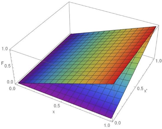
Figure 1. F-x-$\dot{x}$ forces for: ${\alpha }^{*}=0$, i.e., $\alpha =1$ (upper plane), and ${\alpha }^{*}=1$, i.e., $\alpha \to \infty$ (lower plane). Colour in the plot varies with increase of the force F from blue to red.

For ${\alpha }^{*}=0$, the force corresponds to a linear elastic one and is independent of $\dot{x},$ while for ${\alpha }^{*}=1$, the force has a quadratic nonlinearity, which is the product of linear displacement and linear velocity, i.e., $F=kx\dot{x}$. All forces for ${\alpha }^{*}=\left(0,1\right)$ are inside these two boundary ones.

For computational reasons, let us rewrite the force equation (Equation (1)) as

$$F=kx{\left|\dot{x}\right|}^{1-\frac{1}{\alpha }}$$

(5)

where ${\alpha }^{*}=\frac{\alpha -1}{\alpha }$ and $\alpha$ is an integer or non-integer, i.e., $\alpha \in R, \alpha =\left[1,\infty \right)$.

3. Mathematical Model of the Oscillator

Using expression (6), the oscillator is modeled as

$$m\ddot{x}+kx{\left|\dot{x}\right|}^{\frac{\alpha -1}{\alpha }}=0$$

(6)

$$x\left(0\right)=0, \dot{x}\left(0\right)={\dot{x}}_0$$

(7)

where m is a constant. For oscillator (6), the first integral exists.

$$c^2\frac{x^2}{2}+\frac{\alpha }{\alpha +1}{\left|\dot{x}\right|}^{\frac{\alpha +1}{\alpha }}=\frac{\alpha }{\alpha +1}{\left|{\dot{x}}_0\right|}^{\frac{\alpha +1}{\alpha }}$$

(8)

where $c^2=\frac{k}{m}$. Analyzing (5), the boundary phase trajectories are defined.

$$-{\dot{x}}_0\le \dot{x}\le {\dot{x}}_0,-\sqrt{\frac{2\alpha }{\alpha +1}\frac{1}{c^2}{\left|{\dot{x}}_0\right|}^{\frac{\alpha +1}{\alpha }}}\le x\le \sqrt{\frac{2\alpha }{\alpha +1}\frac{1}{c^2}{\left|{\dot{x}}_0\right|}^{\frac{\alpha +1}{\alpha }}}$$

(9)

The extreme value of initial velocity is equal to one, while the extreme displacement depends not only on the initial velocity but also on the order of nonlinearity and rigidity parameter c.

Two different cases can be distinguished:

$${\dot{x}}_0<{(\frac{2\alpha }{\alpha +1})}^{\frac{\alpha }{\alpha -1}}, \sqrt{\frac{2\alpha }{\alpha +1}\frac{1}{c^2}{\left|{\dot{x}}_0\right|}^{\frac{\alpha +1}{\alpha }}}\le \left|x_{max}\right|<\frac{{\dot{x}}_0}{c}$$

(10)

$${\dot{x}}_0>{(\frac{2\alpha }{\alpha +1})}^{\frac{\alpha }{\alpha -1}}, \frac{{\dot{x}}_0}{c}<\left|x_{max}\right|\le \sqrt{\frac{2\alpha }{\alpha +1}\frac{1}{c^2}{\left|{\dot{x}}_0\right|}^{\frac{\alpha +1}{\alpha }}}$$

(11)

The limiting phase trajectories (10) and (11) for various values of α are shown in Figure 2a,b, respectively. It is obtained that if $\alpha \to \infty$ and ${\dot{x}}_0<1$, the lower limit of x tends to zero and the phase trajectory compresses along the horizontal axes, while for ${\dot{x}}_0>1$, the upper limit tends to infinity and the phase trajectory extends along the horizontal axes. In addition, if α$\to$1 and ${\dot{x}}_0<1$, it is inf$\left|x_{max}\right|\to \frac{{\dot{x}}_0}{c}$, while for ${\dot{x}}_0>1$, sup$\left|x_{max}\right|\to \frac{{\dot{x}}_0}{c}$. However, the main conclusion is that the $\dot{x}-x$ diagrams are closed orbits, which correspond to periodical motion.

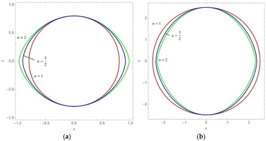
Figure 2. $\dot{x}-x$ diagrams for $c=1$, various values of α, and (a) ${\dot{x}}_0=0.8$ and (b) ${\dot{x}}_0=2.5$.

Transforming (8), we have:

$$dt=\frac{dx}{{({\left|{\dot{x}}_0\right|}^{\frac{\alpha +1}{\alpha }}-\frac{\alpha +1}{\alpha }{c}^2\frac{x^2}{2})}^{\frac{\alpha }{\alpha +1}}}$$

(12)

Integrating (12) in the interval [0, A], where A is the amplitude of vibration, the period of the function is:

$$T=\frac{4}{{\dot{x}}_0}\underset{0}{\overset{A}{{\displaystyle \int }}}\frac{dx}{{(1-\frac{\alpha +1}{2\alpha }{c}^2{\left|{\dot{x}}_0\right|}^{-\frac{\alpha +1}{\alpha }}{x}^2)}^{\frac{\alpha }{\alpha +1}}}$$

(13)

For computational reasons, let us introduce the new variable $u=p^2{x}^2$, where:

$$p^2=\frac{\alpha +1}{2\alpha }{c}^2{\left|{\dot{x}}_0\right|}^{-\frac{\alpha +1}{\alpha }}$$

(14)

Relation (10) is modified into $T=\frac{4}{{\dot{x}}_0}{{\displaystyle \int }}_0^{p^2{A}^2}\frac{du}{2p\sqrt{u}{(1-u)}^{\frac{\alpha }{\alpha +1}}}$. For $p^2{A}^2=1$, i.e.,

$$A=\frac{{\left|{\dot{x}}_0\right|}^{\frac{\alpha +1}{2\alpha }}}{c}\sqrt{\frac{2\alpha }{\alpha +1}}$$

(15)

and using the definition of the complete beta B function [32], $B\left(m,n\right)={{\displaystyle \int }}_0^1{u}^{m-1}{(1-u)}^{n-1}du,$ the period of vibration follows as:

$$T=\sqrt{\frac{2\alpha }{\alpha +1}}\frac{2B(\frac{1}{2},\frac{1}{\alpha +1})}{c{\left|{\dot{x}}_0\right|}^{\frac{\alpha -1}{2\alpha }}}$$

(16)

Analyzing (15) and (16), it is obtained that the amplitude and period of vibration depend on the parameter and order of nonlinearity, but also on the initial velocity.

4. Closed-Form Exact Analytic Solution for Oscillator

Let us assume the exact solution of (6) with initial conditions (7) in the form of the inverse beta function usually called the Ateb function [32].

$$x=A\mathrm{sa}\left(1,\alpha ,\omega t+\theta \right)$$

(17)

where sa$\left(1,\alpha ,\omega t+\theta \right)=\mathrm{sa}$ is the sine Ateb function, ω is the frequency of the function, and A and θ are arbitrary constants. Using the properties of the Ateb function, the first and the second time derivatives of (17) are (see [32]), respectively:

$$\dot{x}=A\omega {\mathrm{ca}}^{\alpha }\left(1,\alpha ,\omega t+\theta \right)$$

(18)

$$\ddot{x}=-\frac{2\alpha }{\alpha +1}{\omega }^{2}Ac{a}^{\alpha -1}\left(1,\alpha ,\omega t+\theta \right)\mathrm{sa}\left(1,\alpha ,\omega t+\theta \right)$$

(19)

where ca($1,\alpha ,\omega t+\theta$) = ca is the cosine Ateb function. Substituting (17) and (19) into (6):

$${\mathrm{ca}}^{\alpha -1}\mathrm{sa}: \omega ={(\frac{\alpha +1}{2\alpha }{c}^2)}^{\frac{\alpha }{\alpha +1}}{A}^{\frac{\alpha -1}{\alpha +1}}$$

(20)

Relation (19) is the frequency of the Ateb function, which depends on the amplitude A. According to the initial conditions (7) and relations (17) and (18), the arbitrary constants satisfy the relations.

$$\theta =0$$

(21)

$${(\frac{\alpha +1}{2\alpha }{c}^2)}^{\frac{\alpha }{\alpha +1}}{A}^{\frac{2\alpha }{\alpha +1}}={\dot{x}}_0$$

(22)

Comparing amplitude (22) with the previously obtained one (12), it is evident that the relations are equal. Substituting (22) into (20), the frequency of the Ateb function is:

$$\omega =c{\left|{\dot{x}}_0\right|}^{\frac{\alpha -1}{2\alpha }}\sqrt{\frac{\alpha +1}{2\alpha }}$$

(23)

Using (23) and the period of the Ateb function [32], $2\mathsf{\Pi }=2B\left(\frac{1}{2},\frac{1}{\alpha +1}\right)$, we obtain the period of vibration of the oscillator (6) as $T=\frac{2\mathsf{\Pi }}{\omega }$, i.e., as is already obtained in (16). Based on the known period of vibration (16) and frequency of the Ateb function (19), the frequency of vibration of the oscillator $\mathsf{\Omega }=\frac{2\pi }{T}=\frac{\pi }{\mathsf{\Pi }}\omega$ follows as:

$$\mathsf{\Omega }=\frac{\pi }{\mathsf{\Pi }}{(\frac{\alpha +1}{2\alpha }{c}^2)}^{\frac{\alpha }{\alpha +1}}{A}^{\frac{\alpha -1}{\alpha +1}}=\frac{\pi }{\mathsf{\Pi }}c{\left|{\dot{x}}_0\right|}^{\frac{\alpha -1}{2\alpha }}\sqrt{\frac{\alpha +1}{2\alpha }}$$

(24)

where $\mathsf{\Pi }=B\left(\frac{1}{2},\frac{1}{\alpha +1}\right)=\frac{\mathsf{\Gamma }\left(\frac{1}{2}\right)\mathsf{\Gamma }\left(\frac{1}{\alpha +1}\right)}{\mathsf{\Gamma }\left(\frac{1}{2}+\frac{1}{\alpha +1}\right)}$ and Γ is the gamma function [32]. It is obvious that the frequency of vibration depends on the amplitude of vibration, i.e., on the initial velocity.

In Figure 3, the A–${\dot{x}}_0$ (22) and the Ω − ${\dot{x}}_0$ (24) diagrams for c = 1 and various values of α are plotted. It is obvious that for $\alpha >1,$ both amplitude and frequency are increasing with the increase in the initial velocity ${\dot{x}}_0$. However, in Figure 3a, two regions for A–${\dot{x}}_0$ variation are evident: first, for ${\dot{x}}_0<{\dot{x}}_{0b}$, and second, for ${\dot{x}}_0>{\dot{x}}_{0b}$, where ${\dot{x}}_{0b}={(\frac{2\alpha }{\alpha +1})}^{\frac{\alpha }{\alpha -1}}$. In the first region, the amplitude of vibration is increasing faster for higher values of $\alpha$, while in the second region, the increase is faster for smaller values of $\alpha$. This result corresponds to (10) and (11), which is already obtained due to qualitative analyses. In Figure 3b, it is shown that the increase in the curves Ω–${\dot{x}}_0$ is higher for smaller values of $\alpha$.

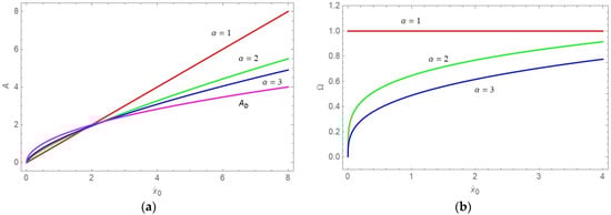
Figure 3. (a) Boundary A_b and A − ${\dot{x}}_0$ curves; (b) $\mathsf{\Omega }-{\dot{x}}_0$ curves for various values of α.

Substituting (20) and (21) into (17), the exact closed-form solution of (6) for (7) is obtained as:

$$x=A\mathrm{sa}(1, \alpha , t(\frac{\alpha +1}{2\alpha }{c}^2{)}^{\frac{\alpha }{\alpha +1}}{A}^{\frac{\alpha -1}{\alpha +1}})$$

(25)

In Figure 4a,b, the x − t diagrams for solutions $A=1$, $c=1$, and $\alpha =1.5,$ i.e., ${\alpha }^{*}=1/3$ and $\alpha =2.5,$ i.e., ${\alpha }^{*}=3/5$, are plotted. It is obvious that the period of vibration is longer for higher values of α, i.e., ${\alpha }^{*}$. Namely, the oscillator with a mixed-form restitution force has a lower frequency of vibration than the elastic oscillator.

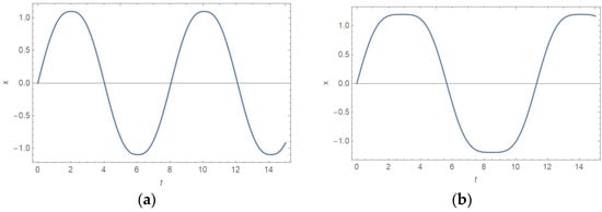
Figure 4. $x-t$ diagrams for A = 1, c = 1, and (a) $\alpha =1.5$, i.e., ${\alpha }^{*}=\frac{1}{3}$; (b) $\alpha =2.5$, i.e., ${\alpha }^{*}=\frac{3}{5}$.

5. Approximate Procedure for Solving the Perturbed Oscillator

Let us consider the perturbed version of Equation (6).

$$\ddot{x}+c^{2}x{\left|\dot{x}\right|}^{\frac{\alpha -1}{\alpha }}=\epsilon f\left(x,\dot{x}\right)$$

(26)

where $f\left(x,\dot{x}\right)$ is a perturbation function and ε << 1 is a small parameter. For ε = 0, Equation (26) transforms into Equation (6). Thus, it follows that Equation (6) is the generating equation for the trial one (26). In accordance with this conclusion, let us assume that the trial solution of (23) has to be the perturbed version of the generating solution (17) of Equation (6). It is supposed that the form of the solution of (26) and its time variable has to be equal to (17) and (18), but with time-variable amplitude and phase.

$$x=A\left(t\right)\mathrm{sa}\left(1,\alpha ,\psi \left(t\right)\right)$$

(27)

$$\dot{x}=A\left(t\right)\omega \left(t\right){\mathrm{ca}}^{\alpha }(\alpha ,1, \psi \left(t\right))$$

(28)

where:

$$\dot{\psi }\left(t\right)=\omega \left(t\right)+\dot{\theta }\left(t\right),$$

(29)

$$\omega \left(t\right)={(\frac{\alpha +1}{2\alpha }{c}^2)}^{\frac{\alpha }{\alpha +1}}A{\left(t\right)}^{\frac{\alpha -1}{\alpha +1}}$$

(30)

$A\left(t\right)$ and $\theta \left(t\right)$ are time-variable functions. Comparing (28) and the time derivative (27), the following constraint is obtained.

$$\dot{A}\left(t\right)\mathrm{sa}+A\left(t\right)\dot{\theta }\left(t\right) {\mathrm{ca}}^{\alpha }=0$$

(31)

where $A\left(t\right)=A,\psi \left(t\right)=\psi ,\theta \left(t\right)=\theta ,\omega \left(t\right)=\omega , \mathrm{sa}\left(1,\alpha ,\psi \left(t\right)\right)=\mathrm{sa}, \mathrm{ca}\left(\alpha ,1,\psi \left(t\right)\right)=\mathrm{ca}.$ Substituting the time variable of (28):

$$\ddot{x}=\left(\dot{A}\left(t\right)\omega \left(t\right)+A\left(t\right)\dot{\omega }\left(t\right)\right){\mathrm{ca}}^{\alpha }-\frac{2\alpha }{\alpha +1}A\left(t\right)\omega \left(t\right)\dot{\psi }\left(t\right){\mathrm{ca}}^{\alpha -1}\mathrm{sa}$$

(32)

and expressions (27) and (28) into (26), it follows that:

$$\left(\dot{A}\left(t\right)\omega \left(t\right)+A\left(t\right)\dot{\omega }\left(t\right)\right){\mathrm{ca}}^{\alpha }-\frac{2\alpha }{\alpha +1}A\left(t\right)\omega \left(t\right)\dot{\theta }\left(t\right){\mathrm{ca}}^{\alpha -1}\mathrm{sa}=\epsilon f\left(A\left(t\right)\mathrm{sa}, A\left(t\right)\omega \left(t\right){\mathrm{ca}}^{\alpha }\right)$$

(33)

Using (30) and the expression:

$$\dot{A}\left(t\right)\omega \left(t\right)+A\left(t\right)\dot{\omega }\left(t\right)=\frac{2\alpha }{\alpha +1}\dot{A}\left(t\right)\omega \left(t\right)$$

(34)

the relation (33) transforms into

$$\dot{A}\left(t\right){\mathrm{ca}}^{\alpha }-A\left(t\right)\dot{\theta }\left(t\right){\mathrm{ca}}^{\alpha -1}\mathrm{sa}=\frac{\alpha +1}{2\alpha \omega \left(t\right)}\epsilon f\left(A\left(t\right)\mathrm{sa}, A\left(t\right)\omega \left(t\right){\mathrm{ca}}^{\alpha }\right)$$

(35)

After some modification, Equations (31) and (35) are rewritten into two first-order differential equations.

$$\dot{A}\left(t\right)=\frac{\alpha +1}{2\alpha \omega \left(t\right)}\epsilon f\left(A\left(t\right)\mathrm{sa}, A\left(t\right)\omega \left(t\right){\mathrm{ca}}^{\alpha }\right)\mathrm{ca}$$

(36)

$$A\left(t\right)\dot{\theta }\left(t\right)=-\frac{\alpha +1}{2\alpha \omega \left(t\right)}\epsilon f\left(A\left(t\right)\mathrm{sa}, A\left(t\right)\omega \left(t\right){\mathrm{ca}}^{\alpha }\right){\mathrm{saca}}^{1-\alpha }$$

(37)

Unfortunately, there does not exist an exact analytic solution for systems (36) and (37). At this point, this is where the averaging of the equations over the period of the Ateb function is introduced. The averaged equations are

$$\dot{A}\left(t\right)=\frac{\alpha +1}{2\alpha \omega \left(t\right)}⟨\epsilon f\left(A\left(t\right)\mathrm{sa}, A\left(t\right)\omega \left(t\right){\mathrm{ca}}^{\alpha }\right)\mathrm{ca}⟩$$

(38)

$$A\left(t\right)\dot{\theta }\left(t\right)=-\frac{\alpha +1}{2\alpha \omega \left(t\right)}⟨\epsilon f\left(A\left(t\right)\mathrm{sa}, A\left(t\right)\omega \left(t\right){\mathrm{ca}}^{\alpha }\right){\mathrm{saca}}^{1-\alpha }⟩$$

(39)

where $⟨·⟩=\frac{1}{T}{\int }_0^T\left(·\right)dt$.

To prove the accuracy of the model, two examples are considered where the approximate analytic solution is compared with the exact numerical solution.

6. Discussion on Perturbed Oscillators

The suggested analytical procedure is applied for solving vibrations of the perturbed oscillators: oscillator with linear damping force and oscillator with additional elastic force.

6.1. Oscillator with External Linear Viscous Damping

For the case when, on the oscillator, an additional viscous damping force $\epsilon f=-\epsilon \dot{x}$ acts, the differential equation of motion is:

$$\ddot{x}+c^{2}x{\left|\dot{x}\right|}^{\frac{\alpha -1}{\alpha }}=-\epsilon \dot{x}$$

(40)

Using the previously mentioned analytic solving procedure, the corresponding averaged equations (Equations (38) and (39)) are:

$$\dot{A}\left(t\right)=-\frac{\alpha +1}{2\alpha }\epsilon A\left(t\right)⟨{\mathrm{ca}}^{\alpha +1}⟩,$$

(41)

$$\dot{\theta }\left(t\right)=\epsilon \frac{\alpha +1}{2\alpha }⟨\mathrm{sa} \mathrm{ca}⟩$$

(42)

using the relation (see [32]):

$${\mathrm{sa}}^2+{\mathrm{ca}}^{\alpha +1}=1$$

(43)

The value of the averaged Ateb function $⟨{\mathrm{sa}}^2⟩=\frac{\alpha +1}{3+\alpha }$, and after integrating (41), it is obtained that the amplitude is an exponential decreasing time function.

$$A\left(t\right)=A\exp \left(-\epsilon \frac{\alpha +1}{\alpha \left(3+\alpha \right)}t\right)$$

(44)

According to (42) and the averaged function $⟨\mathrm{sa} \mathrm{ca}⟩=0$, it follows that

$$\dot{\theta }\left(t\right)=0$$

(45)

$$\dot{\psi }={(\frac{\alpha +1}{2\alpha }{c}^2)}^{\frac{\alpha }{\alpha +1}}{A}^{\frac{\alpha -1}{\alpha +1}}\exp \left(-\epsilon \frac{\alpha +1}{\alpha \left(3+\alpha \right)}t\right).$$

(46)

Integrating (46) and substituting relation (24), the amplitude–time and phase–time relations are obtained.

$$A\left(t\right)=\frac{{\left|{\dot{x}}_0\right|}^{\frac{\alpha +1}{2\alpha }}}{c}\sqrt{\frac{2\alpha }{\alpha +1}}\exp \left(-\epsilon \frac{\alpha +1}{\alpha \left(3+\alpha \right)}t\right)$$

(47)

$$\psi =\sqrt{\frac{\alpha +1}{2\alpha }}c{\left|{\dot{x}}_0\right|}^{\frac{\alpha -1}{2\alpha }}/\left(\epsilon \frac{\alpha +1}{\alpha \left(3+\alpha \right)}\right)\left(1-\exp \left(-\epsilon \frac{\alpha +1}{\alpha \left(3+\alpha \right)}t\right)\right)$$

(48)

For the special case, when α = 1, Equation (40) transforms into the linear damped oscillator, and the relations (47), (48), and (27) for sa(1,1,$\psi$) = sin$\psi$ give the well-known solution:

$$x=\frac{{\dot{x}}_0}{c}\exp \left(-\frac{\epsilon }{2}t\right)\sin \left(ct\right)$$

(49)

Two numerical examples are considered: (a) for $\alpha =1.5$ and (b) for $\alpha =2.5$, described with mathematical models.

$$\ddot{x}+c^{2}x{\left|\dot{x}\right|}^{\frac{1}{3}}=-\epsilon \dot{x}$$

(50)

$$\ddot{x}+c^{2}x{\left|\dot{x}\right|}^{\frac{3}{5}}=-\epsilon \dot{x}$$

(51)

where ε = 0.1. In Figure 5, the $x-t$ diagrams, obtained numerically, and $A-t$ curves obtained analytically (47) are plotted.

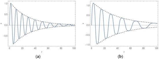
Figure 5. $x-t$ diagrams (full line) and $A-t$ diagrams (dashed line) for damped oscillator with A = 1, c = 1, ε = 0.1, and: (a) $\alpha =1.5$, i.e., ${\alpha }^{*}=\frac{1}{3}$; (b) $\alpha =2.5$, i.e., ${\alpha }^{*}=\frac{3}{5}$.

It is seen that the agreement between numerical and analytical solutions is high even for the long time period. The $A-t$ curves are on the top of the $x-t$ curves.

It is obvious that the amplitude and the period of vibration depend not only on the coefficient of damping but also on the order of nonlinearity: the higher the order of nonlinearity, the slower the velocity of amplitude decrease, and the longer the period of vibration.

6.2. Oscillator with Additional Linear Elastic Term

If an additional linear force $\epsilon f=-\epsilon x$ acts, the equation of motion of the considered oscillator is:

$$\ddot{x}+c^{2}x{\left|\dot{x}\right|}^{\frac{\alpha -1}{\alpha }}=-\epsilon x$$

(52)

The corresponding two first-order averaged differential equations (Equations (38) and (39)) are:

$$\dot{A}\left(t\right)=-\epsilon A\left(t\right)\frac{\alpha +1}{2\alpha \omega \left(t\right)}⟨\mathrm{sa} \mathrm{ca}⟩=0$$

(53)

$$\dot{\theta }\left(t\right)=\epsilon \frac{\alpha +1}{2\alpha \omega \left(t\right)}⟨{\mathrm{sa}}^2{\mathrm{ca}}^{1-\alpha }⟩$$

(54)

i.e., after integration:

$$A\left(t\right)=A=const$$

(55)

$$\psi \left(t\right)=\omega t+\epsilon t\frac{\alpha +1}{2\alpha \omega }⟨{\mathrm{sa}}^2{\mathrm{ca}}^{1-\alpha }⟩$$

(56)

Substituting (30) into (56), the phase angle follows as:

$$\psi \left(t\right)={(\frac{\alpha +1}{2\alpha }{c}^2)}^{\frac{\alpha }{\alpha +1}}{A}^{\frac{\alpha -1}{\alpha +1}}t(1+\epsilon \frac{1}{c^{\frac{4\alpha }{\alpha +1}}}(\frac{\alpha +1}{2\alpha }{)}^{\frac{1-\alpha }{\alpha +1}}{A}^{\frac{2\left(1-\alpha \right)}{\alpha +1}}⟨{\mathrm{sa}}^2{\mathrm{ca}}^{1-\alpha }⟩)$$

(57)

It is obtained that the averaged solution has the constant amplitude (55) while the averaged phase (57) is the linear time function. According to (57) and the periodic property of the Ateb function (see [32]), i.e., $2\mathsf{\Pi }=2B\left(\frac{1}{2},\frac{1}{\alpha +1}\right)$, the period of vibration is:

$$T=\frac{2B\left(\frac{1}{2},\frac{1}{\alpha +1}\right)}{{(\frac{\alpha +1}{2\alpha }{c}^2)}^{\frac{\alpha }{\alpha +1}}{A}^{\frac{\alpha -1}{\alpha +1}}(1+\epsilon \frac{1}{c^{\frac{4\alpha }{\alpha +1}}}(\frac{\alpha +1}{2\alpha }{)}^{\frac{1-\alpha }{\alpha +1}}{A}^{\frac{2\left(1-\alpha \right)}{\alpha +1}}⟨{\mathrm{sa}}^2{\mathrm{ca}}^{1-\alpha }⟩)}$$

(58)

Comparing (58) and (16), i.e., the perturbed case and the unperturbed one (when ε = 0), respectively, it is obvious that the period of vibration is longer for the unperturbed oscillator than for the perturbed one for all values of order of nonlinearity α.

For the case when α = 1, Equation (52) is linear. According to (55), (57), and $⟨{\mathrm{sa}}^2⟩=1/2$, the averaged solution corresponds to the already known one.

$$x=A\sin \left(ct+\frac{\epsilon t}{2c}\right)$$

(59)

Two additional numerical examples are considered where the order of nonlinearity α is 1.5 (Figure 6a) and 2.5 (Figure 6b). The corresponding equations are:

$$\ddot{x}+c^{2}x{\left|\dot{x}\right|}^{\frac{1}{3}}=-\epsilon x$$

(60)

$$\ddot{x}+c^{2}x{\left|\dot{x}\right|}^{\frac{3}{5}}=-\epsilon x$$

(61)

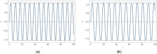
Figure 6. $x-t$ diagrams (full line) and $A-t$ diagrams (dashed line) for A = 1, c = 1, ε = 0.1, and: (a) $\alpha =1.5$, i.e., ${\alpha }^{*}=\frac{1}{3}$; (b) $\alpha =2.5$, i.e., ${\alpha }^{*}=\frac{3}{5}$.

Equations (60) and (61) are solved numerically for $\epsilon =0.1$ and plotted in Figure 6. In addition, the analytically obtained constant amplitude A is inserted into the plot. It is evident that the numerically obtained curves are with constant amplitude A, as is obtained by applying the suggested analytical procedure.

Comparing the period of vibration for the models without elastic force (shown in Figure 4) and that with elastic force (Figure 6), it is seen that the period of vibration is shorter if the elastic force is added, as it is already analytically concluded (see Equation (55)). The shortening of the period of vibration is different for various materials: for those with a higher order of nonlinearity, the influence of the perturbed elastic force is higher and the period of vibration is significantly shorter than for the oscillator without perturbation. The perturbation has no influence on the amplitude of vibration of the oscillator. It remains constant.

7. Conclusions

In the paper, the oscillator with a new type of restitution force is considered. The restitution force is of mixed type and includes the dependence of the material property not only on the strain but also on the strain velocity. Mathematically, the force is of monomial type, i.e., the product of displacement and velocity, and is of integer or non-integer order. The corresponding model of the oscillator is a strong nonlinear differential equation. Analyzing the equation, it is concluded that:

• For the known initial velocity, the model has a constant first integral, which indicates the periodicity of motion. Based on the first integrals, the frequency and amplitude of vibration are obtained.
• There exists the closed-form analytic solution for the oscillator in the form of the sine Ateb function.
• Based on the exact solution, it is concluded that the amplitude, period, and frequency property of the oscillator depend not only on the coefficient and order of nonlinearity of the restitution force, but also on the initial velocity. The amplitude and the frequency of vibration are increasing with initial velocity independently on the order of nonlinearity. The period of vibration of the oscillator is longer for a higher order of nonlinearity, i.e., higher order of velocity of vibration in the restitution force.
• For the perturbed differential equation of the oscillator, the approximate solving procedure with a time-variable amplitude and phase of the sine Ateb function is convenient to be developed. The averaged analytic solution shows good agreement with the numerically obtained one. It proves the accuracy of the procedure developed in the paper.

In addition, it is concluded that the closed-form solution and the developed solving procedure are suitable for prediction of the motion of any oscillators with mixed-type restitution force and for simulation of oscillator responses.

References

- Chen, Z.; Li, J.; Wang, J.; Wa ng, S.; Zhao, J.; Li, J. Towards Hybrid Gait Obstacle Avoidance for a Six Wheel-Legged Robot with Payload Transportation. J. Intell. Robot. Syst. 2021, 102, 21. [Google Scholar] [CrossRef]
- Chen, Z.; Li, J.; Wang, S.; Wang, J.; Ma, L. Flexible gait transition for six wheel-legged robot with unstructured terrains. Rob. Auton. Syst. 2022, 150, 103989. [Google Scholar] [CrossRef]
- Kaviya, B.; Suresh, R.; Chandrasekar, V.K. Extreme bursing events via pulse-shaped explosion in mixed Rayleigh-Lienarrd nonlinear oscillator. Eur. Phys. J. Plus 2022, 137, 844. [Google Scholar] [CrossRef]
- Horváth, R.; Cveticanin, L.; Ninkov, I. Prediction of surface roughness in turning applyins the model of nonlinear oscillator with complex deflection. Mathematics 2022, 10, 12. [Google Scholar] [CrossRef]
- Kakou, P.; Barry, O. Simultaneous vibration reduction and energy harvesting of a nonlinear oscillator using a nonlinear electromagnetic vibration absorber-inerter. Mech. Syst. Signal. Process. 2021, 156, 107607. [Google Scholar] [CrossRef]
- Soares, G.C.; Patnamsetty, M.; Peura, P.; Hokka, M. Effects of adiabatic heating and strain rate on the dynamic response of a CoCrFeMnNi high-entropy alloy. J. Dyn. Behav. Mater. 2019, 5, 320–330. [Google Scholar] [CrossRef]
- Guo, P.; Tang, Q.; Li, L.; Xie, C.; Liu, W.; Zhu, B.; Liu, X. The deformation mechanism and adiabatic shearing behavior of extruded Mg-8.0Al-0.1Mn alloy in different heat treated states under highspeed impact load. J. Mater. Res. Technol. 2021, 11, 2195–2207. [Google Scholar] [CrossRef]
- Gray, G.T. High-strain-rate deformation: Mechanical behavior and deformation substructures induced. Annu. Rev. Mat. Res. 2012, 42, 285–303. [Google Scholar] [CrossRef]
- Peterson, L.A.; Horstemeyer, M.F.; Lacy, T.E.; Moser, R.D. Experimental characterization and constitutive modeling of an aluminum 7085-T711 alloy under large deformations at varying strain rates, stress states, and temperatures. Mech. Mater. 2020, 151, 103602. [Google Scholar] [CrossRef]
- Yakovtseva, O.A.; Kishchik, A.A.; Cheverikin, V.V.; Kotov, A.D.; Mikhaylovskaya, A.V. The mechanisms of the high-strain-rate superplastic deformation of Al-Mg-based alloy. Mater. Lett. 2022, 325, 132883. [Google Scholar] [CrossRef]
- Li, X.; Kim, J.; Roy, A.; Ayvar-Soberanis, S. High temperature and strain-rate response of AA2124-SiC metal matrix composites. Mater. Sci. Eng. A 2022, 856, 144014. [Google Scholar] [CrossRef]
- Natesan, E.; Ahlstrom, J.; Manchili, S.K.; Eriksson, S.; Persson, C. Effect of strain rate on the deformation behavior of A356-T7 cast Aluminium alloys at elevated temperatures. Metals 2020, 10, 1239. [Google Scholar] [CrossRef]
- Gronostajski, Z.; Niechajowicz, A.; Kuziak, R.; Krawczyk, J.; Polak, S. The effect of the strain rate on the stress—strain curve and microstructure of AHSS. J. Mater. Process. Technol. 2017, 242, 246–259. [Google Scholar] [CrossRef]
- El-Magd, E.; Treppmann, C.; Weisshaupt, H. Localisation of deformation and damage under adiabatic compression. J. De Phys. IV Proc. EDP Sci. 1997, 7, C3-511–C3-516. [Google Scholar] [CrossRef]
- Cheng, W.; Outeiro, J.; Costes, J.P.; M'Saoubi, R.; Karaouni, H.; Astakhov, V. A constitutive model for Ti6Al4V considering the state of stress and strain rate effects. Mech. Mater. 2019, 137, 103103. [Google Scholar] [CrossRef]
- Koerber, H.; Kuhn, P.; Ploeckl, M.; Otero, F.; Gerbaud, P.W.; Rolfes, R.; Camanho, P.P. Experimental characterization and constitutive modeling of the non-linear stress–strain behavior of unidirectional carbon–epoxy under high strain rate loading. Adv. Model. Sim. Eng. Sci. 2018, 5, 17. [Google Scholar] [CrossRef]
- Shariyat, M.; Mohammadjani, R. 3D nonlinear variable strain-rate-dependent-order fractional thermoviscoelastic dynamic stress investigation and vibration of thick transversely graded rotating annular plates/discs. Appl. Math. Model. 2020, 84, 287–323. [Google Scholar] [CrossRef]
- Su, T.; Zhou, H.; Zhao, J.; Liu, Z.; Dias, D. A fractional derivative-based numerical approach to rate-dependent stress–strain relationship for viscoelastic materials. Acta Mech. 2021, 232, 2347–2359. [Google Scholar] [CrossRef]
- Song, Y.; Garzia-Gonzales, D.; Rusinek, A. Constitutive models for dynamic strain aging in metals: Strain rate and temperature dependences on the flow stress. Materials 2020, 13, 1794. [Google Scholar] [CrossRef]
- Hou, X.; Liu, Z.; Wang, B.; Lv, W.; Liang, X.; Hua, Y. Stress-strain curves and modified material constitutive model for Ti-6Al-4V over the wide ranges of strain rate and temperature. Materials 2018, 11, 938. [Google Scholar] [CrossRef]
- Haefliger, S.; Famosi, S.; Kaufmann, W. Influence of quasi-static strain rate on the stress-strain characteristics of modern reinforcing bars. Constr. Build. Mater. 2021, 287, 122967. [Google Scholar] [CrossRef]
- Li, J.; Fu, S.; Wang, W. On time-decay rates off strong solutions for the 3D magnetohydrodynamics equations with nonlinear damping. J. Math. Anal. Appl. 2022, 515, 14. [Google Scholar] [CrossRef]
- Guo, K.; Yang, Q.; Tamura, Y. Crosswind response analysis of structures with generalized Van der Pol-type aerodynamic damping by equivalent nonlinear equation method. J. Wind. Eng. Ind. Aerodyn. 2022, 221, 104887. [Google Scholar] [CrossRef]
- Nicaise, S. Stability properties of dissipative evolution equations with nonautonomous and nonlinear damping. Rend. Mat. Appl 2022, 43, 61–102. [Google Scholar]
- Cveticanin, L.; Herisanu, N.; Ninkov, I.; Jovanovic, M. New closed-form solution for quadratic damped and forced nonlinear oscillator with position-dependent mass: Application in grafted skin modeling. Mathematics 2022, 10, 15. [Google Scholar] [CrossRef]
- Ismail, G.M.; Abul-Ez, M.; Farea, N.M. An accurate analytical solution to strongly nonlinear differential equations. Appl. Math. Inf. Sci. 2020, 14, 141–149. [Google Scholar]
- El-Tantawy, S.A.; Salas, A.H.; Alyousef, H.A.; Alharthi, M.R. Novel exact and approximate solutions to the family of the forced damped Kawahara equation and modeling strong nonlinear waves in a plasma. Chin. J. Phys. 2022, 77, 2454–2471. [Google Scholar] [CrossRef]
- El-Dib, Y.O.; Elgazery, N.S. Periodic solution of the parameteric Gaylord’s oscillator with a non-perturbative approach. Europhys. Lett. 2022, 140, 1–7. [Google Scholar] [CrossRef]
- Sierra-Porta, D. Analytic approximations to Lienard nonlinear oscillators with modified energy balance method. J. Vib. Eng. Tech. 2022, 8, 713–720. [Google Scholar] [CrossRef]
- Wen, Y.; Chaolu, T.; Wang, X. Solving the initial value problem of ordinary differential equations by Lie group based neural network method. PLoS ONE 2022, 17, e0265992. [Google Scholar] [CrossRef]
- Lu, J. Global residual harmonic balance method for strongly nonlinear oscillator with cubic and harmonic restoring force. J. Low Freq. Noise Vib. Act. Control 2022, 41, 1402–1410. [Google Scholar] [CrossRef]
- Cveticanin, L. Strong Nonlinear Oscillators—Analytical Solutions, Mathematical Engineering, 2nd ed.; Springer: Berlin/Heidelberg, Germany, 2018; ISBN 978-3-319-58825-4. [Google Scholar]
Disclaimer/Publisher’s Note: The statements, opinions and data contained in all publications are solely those of the individual author(s) and contributor(s) and not of MDPI and/or the editor(s). MDPI and/or the editor(s) disclaim responsibility for any injury to people or property resulting from any ideas, methods, instructions or products referred to in the content. |
© 2023 by the author. Licensee MDPI, Basel, Switzerland. This article is an open access article distributed under the terms and conditions of the Creative Commons Attribution (CC BY) license (https://creativecommons.org/licenses/by/4.0/).