Mathematical Modeling of Gas-Solid Two-Phase Flows: Problems, Achievements and Perspectives (A Review)

Abstract

Mathematical modeling is the most important tool for constructing theories of different kinds of two-phase flows. This review is devoted to the analysis of the introduction of mathematical modeling to two-phase flows, where solid particles mainly serve as the dispersed phase. The main problems and features of the study of gas-solid two-phase flows are included. The main characteristics of gas flows with solid particles are discussed, and the classification of two-phase flows is developed based on these characteristics. The Lagrangian and Euler approaches to modeling the motion of a dispersed phase (particles) are described. A great deal of attention is paid to the consideration of numerical simulation methods that provide descriptions of turbulent gas flow at different hierarchical levels (RANS, LES, and DNS), different levels of description of interphase interactions (one-way coupling (OWC), two-way coupling (TWC), and four-way coupling (FWC)), and different levels of interface resolution (partial-point (PP) and particle-resolved (PR)). Examples of studies carried out on the basis of the identified approaches are excluded, and they are also excluded for the mathematical modeling of various classes of gas-solid two-phase flows.

1. Introduction

Continuum flows, which carry dispersed admixtures, include [1,2,3,4] sandstorms, tornadoes, volcanic eruptions, forest fires, and precipitation in the form of hail, snow, etc. Examples of technical devices that use two-phase currents include the paths of solid-fuel jet engines, pneumatic devices, and many others.

Today, we can state that there is continual growth of interest among researchers in the study of two-phase flows. This seems to be due to two factors. First, in recent years, there has been a tremendous growth in the possibilities of both the mathematical and physical (experimental) modeling of two-phase flows. Second, the range of problems under study for various types of two-phase flows is expanding. The second circumstance largely stems from the first circumstance.

This review differs from other reviews on this topic, which have largely been devoted to some narrower problems (for example, the problem of the influence of particles on gas turbulence, the problem of particle clustering, etc.). This review attempts to analyze the state of mathematical modeling in a broader sense. In the review, a classification of two-phase turbulent flows according to particle inertia is constructed. This classification covers almost the entire range of particle inertia. This classification is of great prognostic value since it offers new dimensionless criteria that allow one to analyze both the existing results at different qualitative levels and conduct new studies regarding various classes of two-phase flows determined by the concentration and inertia of particles.

This review is devoted to the analysis of the currently available approaches to the mathematical modeling of two-phase flows, where mainly solid particles act as the dispersed phase. For anyone who is interested in the direct numerical simulation (DNS) of turbulent flows with droplets and bubbles, it is recommended that they refer to the review presented in [5].

This review is structured as follows. Section 2 describes the main problems and the particularity of studying gas-solid two-phase flows. The main characteristics of gas flows with solid particles and the classifications of gas-solid two-phase flows developed on their basis are discussed in Section 3. Section 4 describes Lagrangian and Eulerian approaches to modeling the motion of the dispersed phase and discusses issues relating to the mathematical modeling of a gas flow that carries particles. The final section, Section 5, presents modern numerical modeling methods that describe turbulent gas flow at different hierarchical levels, different descriptive levels of interphase interactions, and different levels of resolution of the interphase boundary.

2. Main Problems and Specific Features of Two-Phase Flow Modeling

2.1. Main Problems of Two-Phase Flow Modeling

Heterogeneous or two-phase flows are studied to solve two main problems [6,7].

2.2. Specific Features of Two-Phase Flow Modeling

2.2.1. Multiscale Physics of Two-Phase Flow

The inertia of particles (which is primarily determined by their size and density) can vary in a colossal range (many orders of magnitude). One-phase flows are characterized by a number of space-time scales that are determined by the magnitude of their inherent flow velocity, flow regime (laminar, transient, and turbulent), flow geometry, etc. For the accurate modeling of particle motion, it is necessary to consider particles’ interactions at different scales; these interactions are determined by (1) averaged movement, (2) wide-scale fluctuation motions, (3) fine-scale fluctuation motions, (4) different instabilities (for example, Tollmin–Schlichting instability in boundary layers, Taylor–Gertler instability in pipes, and Kelvin–Helmholtz instability in pure shear layers), etc.

2.2.2. Multiplicity of Forces Acting on Particles

For the correct integration of the equations of a particle’s motion, it is necessary to consider a large number of force factors (forces). The main forces are listed as follows: (1) aerodynamic drag force, (2) gravitational forces (Archimedes forces), (3) Safmans’ force, (4) Magnus’ force, (5) the force of thermophoresis, (6) the force of turbofreezing, (7) the force of diffusiophoresis, (8) centrifugal force, (9) electrostatic forces, and (10) wall power.

It important to notice that many of these forces, in one form or another, contain the velocity of the carrier phase $\mathbf{u}(\tau )$, which is a random variable in a turbulent flow. Therefore, a question often arises regarding the applicability of a particular expression that is obtained theoretically or empirically for other conditions to calculating the influence of forces (for example, for laminar flow or in the absence of velocity shift).

2.2.3. Multiplicity of Modeling Parameters

The main parameters are as follows: (1) three components of the average speed ($U_i$, $U_j$, and $U_k$), (2) three components of the fluctuation (rms) velocity (${(\overline{{u_i^{\prime }}^2})}^{1/2}$, ${(\overline{{u_j^{\prime }}^2})}^{1/2}$, and ${(\overline{{u_k^{\prime }}^2})}^{1/2}$), (3) average temperature (T), (4) fluctuation (rms) in temperature (${(\overline{{t^{\prime }}^2})}^{1/2}$), (5) double correlations of various components of fluctuation velocities (components of the Reynolds stress tensor) ($\overline{u_i^{\prime }{u}_j^{\prime }}$), (6) double correlations of fluctuation velocity and fluctuation temperature ($\overline{u_i^{\prime }\hspace{0.17em}{t}^{\prime }}$, $\overline{u_j^{\prime }\hspace{0.17em}{t}^{\prime }}$), etc.

This multiplicity is explained by the fact that similar parameters for the dispersed phase are added to the parameters indicated above (for example, averaged ($V_i$, $V_j$, $V_k$) and fluctuation velocities (${(\overline{{v_i^{\prime }}^2})}^{1/2}$, ${(\overline{{v_j^{\prime }}^2})}^{1/2}$, and ${(\overline{{v_k^{\prime }}^2})}^{1/2}$) and particle temperatures ($T_p$, ${(\overline{{t_p^{\prime }}^2})}^{1/2}$), etc.), including their size, size distribution, averaged and fluctuation (rms) concentrations ($\mathsf{\Phi }$, ${(\overline{{{\varphi }^{\prime }}^2})}^{1/2}$), and the parameters for the carrier phase (in the presence of particles), the heat of phase transitions, and many others.

2.2.4. Multiplicity of Collision Processes

The main factors contributing to the occurrence of collisions between particles are listed as follows: (1) polydispersity, which leads to a difference in the averaged velocities; (2) the influence of the gradient of the averaged velocity of the carrier phase; (3) the influence of gravity (Archimedes); (4) the turbulent transport effect, which leads to the appearance of relative velocity between nearby particles; (5) the effect of clustering, i.e., an increase in the concentration of the dispersed phase in local regions of space; (6) electrostatic interactions; and (7) Brownian motion.

2.2.5. Multiplicity of Phase and Chemical Transformations

Phase transformations are not considered in this review because the subject of this review is gas flows with solid particles (gas-solid two-phase flow). However, for non-isothermal two-phase flows, particle melting may occur during interphase heat exchange. The melting of particles in the gas stream leads to the transition of a gas-solid two-phase flow into a gas–liquid two-phase flow. The subsequent process of the crystallization (solidification) of droplets can cause the flow to “return” to its initial state.

2.2.6. Multiplicity of Dimensionless Parameters

An example of such parameters is represented by the numerous Stokes numbers (see Section 3.3) that characterize the inertia of the dispersed phase with ratios of the various scales of the carrier gas, the Reynolds number of the particle, etc.

3. Main Characteristics of Two-Phase Flows

This section presents classifications of two-phase flows developed on their basis.

3.1. Particle Concentrations

The possible varieties of particle concentrations (classification) are given in [8,9]. There are three classes of two-phase flows: (1) dilute two-phase flows without the reverse effect of the dispersed phase; (2) dilute two-phase flows with the reverse effect of the dispersed phase; and (3) dense two-phase flows with intense collisional interactions between particles.

3.1.1. One-Way Coupling

To model the motion of particles in dilute two-phase streams (dispersed phase $\mathsf{\Phi }\le 10^{-6}$), that is, streams with a small Φ, “one-way coupling” (OWC) is applied.

3.1.2. Two-Way Coupling

With an increase in the concentration of particles (${10}^{-6}<\mathsf{\Phi }\le {10}^{-3}$) [10,11,12,13,14], “two-way coupling” (TWC) occurs.

3.1.3. Four-Way Coupling

Further growth ($\mathsf{\Phi }>10^{-3}$) requires the inclusion of the contribution of interparticle interactions to the process of the momentum and energy transfer of the dispersed phase [15,16,17,18]. The chaotic motion of particles during their interaction is called “pseudoturbulence” to distinguish it from the actual turbulent fluctuations of particle velocities associated with their involvement in the turbulent motion of the carrier flow.

It should be noted that there is a clustering phenomenon in two-phase flows that consists of a sharp increase in the concentration of particles in local areas. This significant rise in Φ leads to an increase in the probability of particle collisions, even in a dilute two-phase flow.

In reference to what has been discussed above, it is clear that in flows with a small mass of dispersed phase content, in which particles do not undergo collisions and do not have a reverse effect on the flow of the carrier continuous medium, clustering phenomena can lead to flow restructuring. The formation of local areas of increased particle concentrations has been revealed experimentally or via calculation in various flows, including homogeneous isotropic turbulence [19,20], shear flows in pipes (channels) [21,22], flows in boundary layers [23], jet flows, traces behind streamlined bodies, flows around blunted bodies [24], and free, concentrated vortices [25,26,27].

3.2. Particles’ Dynamic Relaxation Time

The inertia of particles is the time of dynamic relaxation ${\tau }_p$, which is represented in the following form

$${\tau }_p={\tau }_{p0}/C({\mathrm{Re}}_p)=\frac{{\rho }_p\hspace{0.17em}{d}_p^2}{18\mu \hspace{0.17em}C({\mathrm{Re}}_p)}$$

(1)

where ${\rho }_p$ is the physical density; ${\tau }_{p0}$ is the time of dynamic relaxation of the Stokes particle; $\mu$ is the dynamic viscosity.

3.3. Stokes Numbers

There are three dimensionless criteria listed in [28,29]: ${\mathrm{Stk}}_f$, ${\mathrm{Stk}}_L$, and ${\mathrm{Stk}}_K$, representing Stokes numbers in averaged, large-scale, and small-scale fluctuation movements, respectively.

$${\mathrm{Stk}}_i=\frac{{\tau }_p}{T_i}.$$

(2)

In the equation above, $T_i$ denotes a given characteristic time of the carrier phase.

3.3.1. Stokes Number in Time-Averaged Motion

We can apply the Stokes number to averaged motion, which we express as

$${\mathrm{Stk}}_f=\frac{{\tau }_p}{T_f},$$

(3)

where $T_f$ is the characteristic time of the carrier phase in the averaged motion.

3.3.2. Stokes Number in Large-Scale Fluctuation Motions

In this case, the Stokes number assumes the following form

$${\mathrm{Stk}}_f=\frac{{\tau }_p}{T_L},$$

(4)

where $T_L$ is the characteristic time of the carrier gas in a large–scale fluctuation motion (temporal Lagrangian integral turbulence scale).

3.3.3. Stokes Number in Small-Scale Fluctuation Motions

The inertia of particles in small-scale fluctuation motions can be characterized by the Stokes number we represent as

$${\mathrm{Stk}}_f=\frac{{\tau }_p}{{\tau }_K},$$

(5)

where ${\tau }_K$ is the Kolmogorov time scale of turbulence.

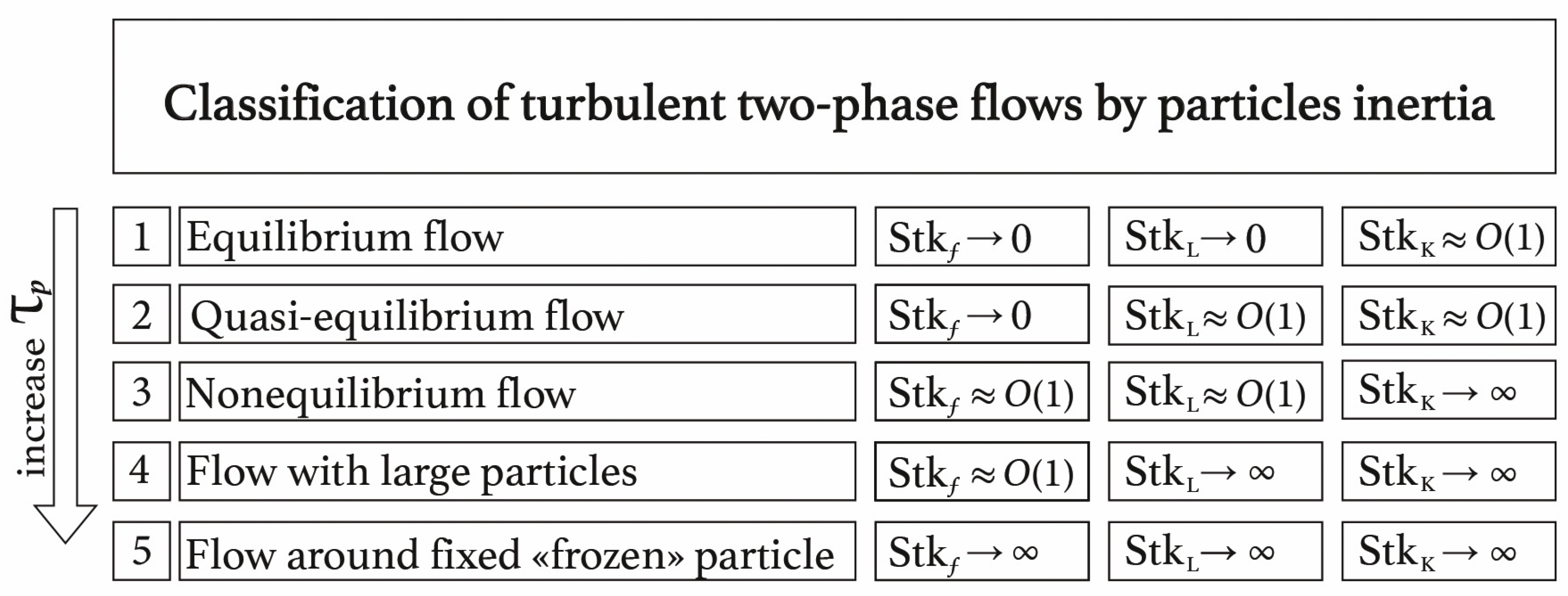
3.4. Classification of Turbulent Two-Phase Flows According to Particle Inertia

We will briefly describe the classification of turbulent two-phase flows according to particle inertia (see Figure 1 and Figure 2) depending on Stokes numbers [28,29].

Flow around fixed “frozen” particles. In this case, the particles have an extremely large amount of inertia, which remains completely static and whose temperature does not change. An analogue of such a hypothetical class of two-phase flows is a one-phase flow in heat exchangers, where fixed pipes act as such particles, through which the working fluid moves.

4. Lagrangian and Eulerian Modeling of Two-Phase Flows

Mathematical modeling methods play an important role in the study of the processes of the motion of solid particles. Detailing a large number of processes in which information about each individual is not always indisputable can lead to a decrease in the reliability of the created model.

4.1. Reasons for Considering of the Two-Phase Nature of Tornados

It is clear that the attempts to describe all the varieties of two-phase flows using all models can hardly be justified. As a consequence, for certain classes of flows (see Section 3), which are characterized primarily by the concentration of the dispersed phase and Stokes numbers, specific models should be preferred.

4.2. Lagrangian Modeling

The system of equations is as follows (example taken from [30])

$$\frac{d{\mathbf{x}}_p}{d\tau }=\mathbf{v},$$

(6)

$$m_p\frac{d\mathbf{v}}{d\tau }={\displaystyle \sum _i{\mathbf{F}}_i}={\mathbf{F}}_D+{\mathbf{F}}_g+{\mathbf{F}}_S+{\mathbf{F}}_M+\dots ,$$

(7)

$$I\frac{d{\mathsf{\omega }}_p}{d\tau }=\mathbf{T},$$

(8)

where ${\mathbf{x}}_p$ is the position vector (radius vector) of the particle, $\mathbf{v}$ is the instantaneous velocity vector of the particle, ${\mathsf{\omega }}_p$ is the angular velocity vector of the particle, $m_p$ is the mass of the particle, and $I$ is the moment of inertia of the particle. Equation (8) describes the change in angular velocity of the particle due to viscous interactions with the surrounding gas.

Due to the viscosity of the liquid, a moment of rotation $\mathbf{T}$ acts on a rotating particle.

4.3. Eulerian Modeling

Let us briefly consider the current approaches to constructing continuum equations for the motion of dispersed impurity and analyze the features of describing their behavior for different classes of two-phase flows.

Algebraic and differential models. There are two main approaches to determining the velocity correlations of dispersed phases. One of them is presented in [31,32]

$$\overline{v_i^{\prime }{v}_j^{\prime }}=A\hspace{0.17em}\overline{u_i^{\prime }{u}_j^{\prime }},$$

(9)

where $A$ is the function of a particle’s involvement in gas fluctuation movement.

The other approach consists of applying gradient relations like the Boussinesq relations for a single-phase flow [33]

$$\overline{v_i^{\prime }{v}_j^{\prime }}=-{\nu }_p\left(\frac{\partial V_i}{\partial x_j}\right),$$

(10)

or in the form presented in [34,35]

$$\overline{v_i^{\prime }{v}_j^{\prime }}=-{\nu }_p\left(\frac{\partial V_i}{\partial x_j}+\frac{\partial V_j}{\partial x_i}-\frac{2}{3}\frac{\partial V_k}{\partial x_k}{\delta }_{ij}\right)+\frac{2}{3}{k}_p{\delta }_{ij},$$

(11)

where ${\nu }_p$ is the turbulent viscosity coefficient of the dispersed phase. Different methods for determining the value of ${\nu }_p$ have been described in the literature [34,35].

Models based on kinetic equations for probability density function (PDF).

The first method. Single-point kinetic equations for the PDF of the velocity and temperature distributions of particles in a turbulent flow using a functional formalism based on the Furutsu–Donsker–Novikov formula for Gaussian random fields were obtained in [36,37,38,39,40,41,42,43,44,45,46,47].

According to this first method, to transform stochastic equations like the Langevin equation into a kinetic equation for a group of particles, a probability density function (PDF) that describes the coordinate $x$, velocity $v$, and temperature distribution of particles $t_p$ is introduced:

$$P(\mathbf{x},\mathbf{v},t_p,\tau )=\overline{\delta (\mathbf{x}-{\mathbf{r}}_p(\tau ))\delta (\mathbf{v}-{\mathbf{v}}_p(\tau ))\delta (t_p-t_p(\tau ))},$$

(12)

where averaging is not carried out over time but over realizations of the random fields of the carrying gas flow.

The equation for the PDF is then used, as presented in [36]:

$$\frac{\partial \mathsf{\Phi }}{\partial \tau }+{\displaystyle \sum _j\frac{\partial \mathsf{\Phi }{V}_j}{\partial x_j}}=0,$$

(13)

$$\frac{\partial V_i}{\partial \tau }+{\displaystyle \sum _j{V}_j\frac{\partial V_i}{\partial x_j}}=-{\displaystyle \sum _j\frac{\partial \overline{v_i^{\prime }{v}_j^{\prime }}}{\partial x_j}}+\frac{U_i-V_i}{{\tau }_p}-{\displaystyle \sum _j\frac{D_{pij}}{{\tau }_p}\frac{\partial \ln \mathsf{\Phi }}{\partial x_j}},$$

(14)

$$\frac{\partial T_p}{\partial \tau }+{\displaystyle \sum _j{V}_j\frac{\partial T_p}{\partial x_j}}=-{\displaystyle \sum _j\frac{\partial \overline{v_j^{\prime }{t}_p^{\prime }}}{\partial x_j}}+\frac{T-T_p}{{\tau }_t}-{\displaystyle \sum _j\frac{D_{pj}^t}{{\tau }_t}\frac{\partial \ln \mathsf{\Phi }}{\partial x_j}},$$

(15)

where $\overline{v_i^{\prime }{v}_j^{\prime }}=\frac{1}{\mathsf{\Phi }}{\displaystyle \iint v_i^{\prime }}{v}_j^{\prime }Pdvd{t}_p$, $\overline{v_j^{\prime }{t}_p^{\prime }}=\frac{1}{\mathsf{\Phi }}{\displaystyle \iint v_j^{\prime }}{t}_p^{\prime }Pdvd{t}_p$, $D_{pij}={\tau }_p(\overline{v_i^{\prime }{v}_j^{\prime }}+g_p\overline{u_i^{\prime }{u}_j^{\prime }})$, $D_{pj}^t={\tau }_t\overline{v_j^{\prime }{t}_p^{\prime }}+{\tau }_p{g}_{pt}\overline{u_j^{\prime }{t}^{\prime }}$, $g_p=T_{pL}/{\tau }_p-1+\exp (-T_{pL}/{\tau }_p)$, $g_{pt}=T_{pLt}/{\tau }_p-1+\exp (-T_{pLt}/{\tau }_p)$.

Here, $T_{pL}$ _and $T_{pLt}$ are the times of interaction between particles (droplets) and energy-intensive fluctuations of velocity and temperature, respectively, for the non-inertial impurities $T_{pL}=T_L$ and $T_{pLt}=T_{Lt}$.

The system of Equations (13)–(15) is not closed, as the equations contain information related to particle involvement in fluctuating motion turbulent stresses $\overline{v_i^{\prime }{v}_j^{\prime }}$ and turbulent heat flux $\overline{v_j^{\prime }{t}_p^{\prime }}$ in the dispersed phase as well as the turbulent diffusion of momentum and heat arising from non-uniform particle concentrations.

A mathematical description of momentum and heat transfer processes in the dispersed phase of varying complexity was developed in [36]:

$$\frac{\partial k_p}{\partial \tau }+{\displaystyle \sum _j{V}_j\frac{\partial k_p}{\partial x_j}=-\frac{1}{\mathsf{\Phi }}{\displaystyle \sum _j\frac{\partial \mathsf{\Phi }\overline{v_i^{\prime }{v}_i^{\prime }{v}_j^{\prime }}}{2\partial x_j}}}-{\displaystyle \sum _j{\displaystyle \sum _i\overline{v_i^{\prime }{v}_j^{\prime }}\frac{\partial V_i}{\partial x_j}}}+\frac{2}{{\tau }_p}(f_{u}k-k_p),$$

(16)

where $k_p=\frac{1}{2}{\displaystyle \sum _i\overline{v_i^{\prime }{v}_i^{\prime }}}$ is the energy of the fluctuations of the dispersed phase velocity.

The second method. The methods presented in [48,49] allow for the acquisition of equations for joint PDF distributions of the velocity and temperature of the dispersed impurity [50].

The third method. The third method constitutes the construction of a closed kinetic equation based on the expansion of the characteristic functional into a series of cumulants [51,52].

4.4. Advantages and Limitations of Lagrangian and Eulerian Modeling

Let us consider Euler–Lagrange and Euler–Euler models with respect to describing the motion of flows of continuous media with solid particles, droplets, and bubbles [36].

The advantage of Euler–Lagrange (trajectory and stochastic) models is their ability to obtain detailed statistical information about the motion of individual particles via integrating the equations of motion.

It should be noted that with an increase in the concentration of the dispersed phase, there are also difficulties in using Euler–Lagrange models [53].

4.5. Description of the Gas Flow Carrying the Particles

An increase in the volume fraction of the dispersed phase can affect the carrier medium (see Section 3.1.2). Let us consider the motion of a continuous medium (gas) in the presence of particles when the particles begin to have a reverse influence on the medium’s characteristics.

4.5.1. Actual Equations

The relevant equations are as follows:

$${\displaystyle \sum _j\frac{\partial u_j}{\partial x_j}}=0,$$

(17)

$$\frac{\partial u_i}{\partial \tau }+{\displaystyle \sum _j{u}_j\frac{\partial u_i}{\partial x_j}}=-\frac{1}{\rho }\frac{\partial p}{\partial x_i}+\nu {\displaystyle \sum _j\frac{{\partial }^2{u}_i}{\partial x_j\partial x_j}}-\frac{{\rho }_p\varphi }{\rho }\frac{(u_i-v_i)}{{\tau }_p},$$

(18)

$$\frac{\partial \hspace{0.17em}t}{\partial \tau }+{\displaystyle \sum _j{u}_j\frac{\partial \hspace{0.17em}t}{\partial x_j}}=a{\displaystyle \sum _j\frac{{\partial }^{2}t}{\partial x_j\partial x_j}}-\frac{C_{p_p}{\rho }_p\varphi }{C_p\rho }\frac{(t-t_p)}{{\tau }_t},$$

(19)

The continuity equation (Equation (17)) has a form similar to the single-phase flow equation.

4.5.2. Time-Averaged Equations

The resulting averaged continuity, motion, and energy equations are expressed as follows:

$${\displaystyle \sum _j\frac{\partial U_j}{\partial x_j}}=0,$$

(20)

$$\frac{\partial U_i}{\partial \tau }+{\displaystyle \sum _j{U}_j\frac{\partial U_i}{\partial x_j}}=-\frac{1}{\rho }\frac{\partial P}{\partial x_i}+\nu {\displaystyle \sum _j\frac{{\partial }^2{U}_i}{\partial x_j\partial x_j}}-{\displaystyle \sum _j\frac{\partial (\overline{u_i^{\prime }{u}_j^{\prime }})}{\partial x_j}}-\frac{{\rho }_p\mathsf{\Phi }}{\rho }\frac{(U_i-V_i)}{{\tau }_p}-\frac{{\rho }_p\overline{{\varphi }^{\prime }{u}_i^{\prime }}}{\rho {\tau }_p},$$

(21)

$$\frac{\partial \hspace{0.17em}T}{\partial \tau }+{\displaystyle \sum _j{U}_j\frac{\partial \hspace{0.17em}T}{\partial x_j}}=a{\displaystyle \sum _j\frac{{\partial }^{2}T}{\partial x_j\partial x_j}}-{\displaystyle \sum _j\frac{\partial (\overline{u_j^{\prime }{t}^{\prime }})}{\partial x_j}}-\frac{C_{p_p}{\rho }_p\mathsf{\Phi }}{C_p\rho }\frac{(T-T_p)}{{\tau }_t}-\frac{C_{p_p}{\rho }_p\overline{{\varphi }^{\prime }{t}^{\prime }}}{C_p\rho {\tau }_t},$$

(22)

Let us assume that the distributions of the averaged velocities and particle concentrations are known. We need to determine the turbulent gas stresses $\overline{u_i^{\prime }{u}_j^{\prime }}$ and the turbulent heat flux $\overline{u_j^{\prime }{t}^{\prime }}$ as well as the correlations between particle concentration fluctuations and gas velocity and temperature fluctuations $\overline{{\varphi }^{\prime }{u}_i^{\prime }}$ and $\overline{{\varphi }^{\prime }{t}^{\prime }}$_, which can be represented as follows [54,55,56]:

$$\overline{{\varphi }^{\prime }{u}_i^{\prime }}=-{\tau }_p{g}_p\overline{u_i^{\prime }{u}_j^{\prime }}\frac{\partial \mathsf{\Phi }}{\partial x_j},$$

(23)

$$\overline{{\varphi }^{\prime }{t}^{\prime }}=-{\tau }_p{g}_{pt}\overline{u_j^{\prime }{t}^{\prime }}\frac{\partial \mathsf{\Phi }}{\partial x_j},$$

(24)

$g_p=T_{pL}/{\tau }_p-1+\exp (-T_{pL}/{\tau }_p)$, $g_{pt}=T_{pLt}/{\tau }_p-1+\exp (-T_{pLt}/{\tau }_p)$.

4.5.3. Equations for the Reynolds Stresses

Subtracting Equations (20)–(22) from Equations (17)–(19) yields the following equations:

$$\begin{array}{l}\frac{\partial (\overline{u_i^{\prime }{u^{\prime }}_j})}{\partial \tau }+{\displaystyle \sum _k{U}_k\frac{\partial (\overline{u_i^{\prime }{u}_j^{\prime }})}{\partial x_k}=}{\displaystyle \sum _k\frac{\partial }{\partial x_k}}\left[\nu \frac{\partial (\overline{u_i^{\prime }{u}_j^{\prime }})}{\partial x_k}-\overline{u_i^{\prime }{u}_j^{\prime }{u}_k^{\prime }}\right]-\\ {\displaystyle \sum _k\left[(\overline{u_j^{\prime }{u}_k^{\prime }})\frac{\partial U_i}{\partial x_k}+(\overline{u_i^{\prime }{u}_k^{\prime }})\frac{\partial U_j}{\partial x_k}\right]}-\frac{1}{\rho }(\overline{u_i^{\prime }\frac{\partial p^{\prime }}{\partial x_j}}+\overline{u_j^{\prime }\frac{\partial p^{\prime }}{\partial x_i}})-2\nu {\displaystyle \sum _k\overline{\frac{\partial u_i^{\prime }\partial u_j^{\prime }}{\partial x_k\partial x_k}}}-\\ \frac{{\rho }_p}{\rho {\tau }_p}[\mathsf{\Phi }(2\overline{u_i^{\prime }{u}_j^{\prime }}-\overline{v_i^{\prime }{u}_j^{\prime }}-\overline{u_i^{\prime }{v}_j^{\prime }})+\overline{{\varphi }^{\prime }{u}_j^{\prime }}(U_i-V_i)+\overline{{\varphi }^{\prime }{u}_i^{\prime }}(U_j-V_j)+\\ (2\overline{{\varphi }^{\prime }{u}_i^{\prime }{u}_j^{\prime }}-\overline{{\varphi }^{\prime }{v}_i^{\prime }{u}_j^{\prime }}-\overline{{\varphi }^{\prime }{u}_i^{\prime }{v}_j^{\prime }})]\end{array}$$

(25)

Equation (25) differs from the corresponding equation of a single-phase flow via the presence of the last group of terms on the right-hand side, which takes into account the dynamic influence of particles on the carrier flow.

The system of Equations (20), (21), (23), and (25) is unclosed because Equation (25) contains unknown triple correlations of velocity fluctuations of the carrier phase, serving as correlations related to fluctuations in particle concentration and velocity.

Algebraic models. These models typically use the semi-empirical theory of turbulence developed by Prandtl [57,58,59].

One-parameter models. The model based on the turbulence energy equation is the most common (as in the case of single-phase flow). It is necessary to multiply the equation of fluctuation motion by $u_i^{\prime }$, sum over $i$, and then average the result. The equation will then have the following form:

$$\begin{array}{l}\frac{\partial k}{\partial \tau }+{\displaystyle \sum _j{U}_j\frac{\partial k}{\partial x_j}}={\displaystyle \sum _j\frac{\partial }{\partial x_j}}\left[\nu \frac{\partial k}{\partial x_j}-\overline{{u^{\prime }}_j\left(\frac{1}{2}{\displaystyle \sum _i{u_i^{\prime }}^2}+\frac{p^{\prime }}{\rho }\right)}\right]-\\ {\displaystyle \sum _j{\displaystyle \sum _i\overline{u_i^{\prime }{u}_j^{\prime }}}}\frac{\partial U_i}{\partial x_j}-\nu {\displaystyle \sum _j{\displaystyle \sum _i\overline{\frac{\partial u_i^{\prime }}{\partial x_j}}}}\overline{\frac{\partial u_i^{\prime }}{\partial x_j}}-\\ {\displaystyle \sum _i\frac{{\rho }_p}{\rho {\tau }_p}\left[\mathsf{\Phi }(\overline{u_i^{\prime }{u}_i^{\prime }}-\overline{u_i^{\prime }{v}_i^{\prime }})+\overline{{\varphi }^{\prime }{u}_i^{\prime }}(U_i-V_i)+(\overline{{\varphi }^{\prime }{u}_i^{\prime }{u}_i^{\prime }}-\overline{{\varphi }^{\prime }{u}_i^{\prime }{v}_i^{\prime }})\right]}\end{array}$$

(26)

The Equation (26) can be rewritten concisely:

$$\frac{Dk}{D\tau }=D+P-\epsilon -{\epsilon }_p,$$

(27)

where the additional dissipation ${\epsilon }_p$_, caused by the presence of a dispersed phase, assumes the following form:

$${\epsilon }_p={\displaystyle \sum _i\frac{{\rho }_p}{\rho {\tau }_p}\left[\hspace{0.17em}\mathsf{\Phi }(\overline{u_i^{\prime }{u}_i^{\prime }}-\overline{u_i^{\prime }{v}_i^{\prime }})+\overline{{\varphi }^{\prime }{u}_i^{\prime }}(U_i-V_i)+(\overline{{\varphi }^{\prime }{u}_i^{\prime }{u}_i^{\prime }}-\overline{{\varphi }^{\prime }{u}_i^{\prime }{v}_i^{\prime }})\right]}.$$

(28)

There have been several studies (e.g., [60,61,62]) in which the authors attempted to estimate the magnitude of the terms on the right-hand side (28) for different classes of two-phase flows. This means the second and third terms on the right-hand side (28) are small compared to the first term. Thus, in the implementation of quasi-equilibrium and non-equilibrium flows (see Figure 1 and Figure 2), the first term on the right-hand side (28) will play a determining role in the process of dissipation:

$${\epsilon }_p={\displaystyle \sum _i\frac{{\rho }_p\mathsf{\Phi }}{\rho {\tau }_p}\overline{u_i^{\prime }{u}_i^{\prime }}=\frac{2\mathrm{M}k}{{\tau }_p}}.$$

(29)

Considering this mechanism [63,64,65] leads to Equation (27) assuming the following form

$$\frac{Dk}{D\tau }=D+P-\epsilon +P_p-{\epsilon }_p,$$

(30)

where $P_p$ is the additional generation caused by the presence of particles.

Two-parameter models. As in the study of single-phase turbulent flows, the two-parameter $k-\epsilon$—turbulence model has become the most widespread.

By analogy with the equation for a single-phase flow in the case of two-phase flow, we obtain

$$\frac{D\epsilon }{D\tau }=D_{\epsilon }+P_{\epsilon }-{\epsilon }_{\epsilon }-{\epsilon }_{\epsilon p}.$$

(31)

where ${\epsilon }_{\epsilon p}$ is the reduction in dissipation due to the presence of particles.

The equation for ${\epsilon }_{\epsilon p}$ is most often represented as follows [66,67]:

$${\epsilon }_{\epsilon p}=C_{\epsilon 3}\frac{\epsilon }{k}{\epsilon }_p,$$

(32)

where the constant $C_{\epsilon 3}$ can assume the following values: $C_{\epsilon 3}=1.0$ [68], $C_{\epsilon 3}=1.2$ [66], and $C_{\epsilon 3}=1.9$ [69].

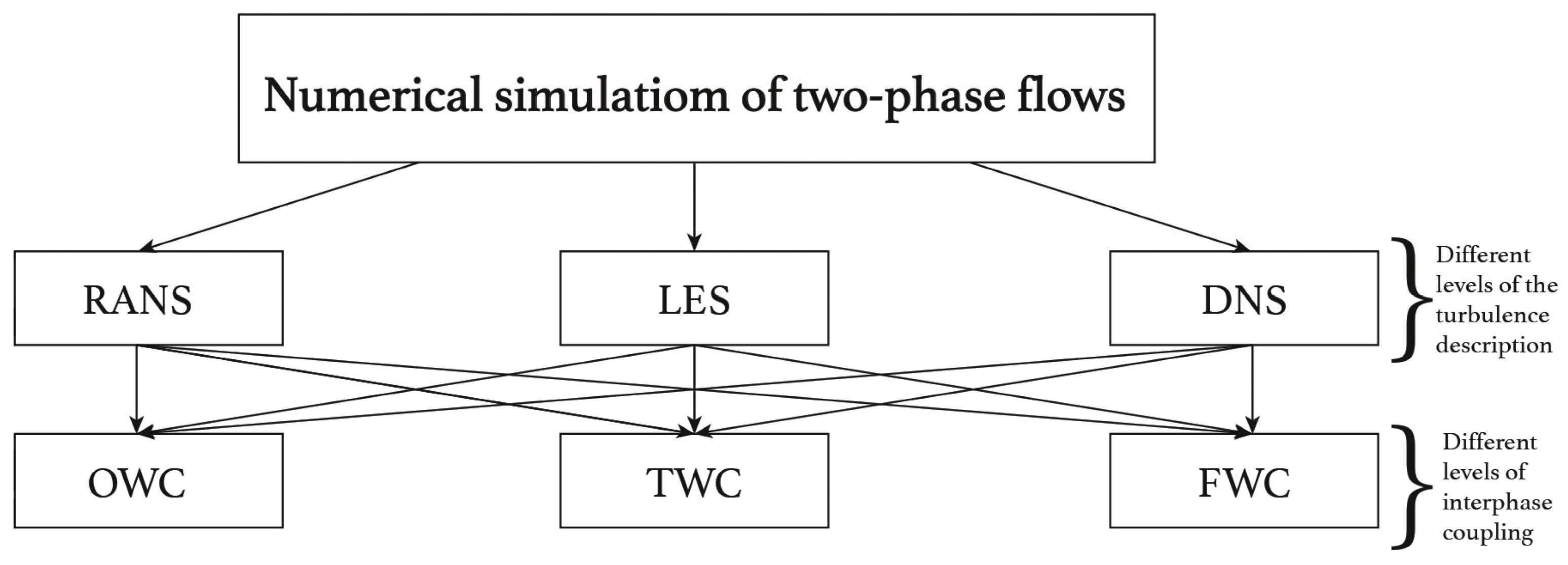
5. Methods of Numerically Modeling Two-Phase Flows

The main methods of numerically modeling two-phase flows are presented below.

5.1. Particle-Resolved DNS

Particle-resolved direct numerical simulation (PR DNS) is the method that most fully describes the physics of two-phase flows. In this method, flow around each particle is allowed to occur. In this case, the behavior of each particle is determined by both external acting forces and the aerodynamic drag force from the carrier gas (determined in the calculation process). This method is also applicable to the calculation of more complex two-phase flows carrying droplets or bubbles, where the interfacial surface may deform. This deformation is calculated using the aerodynamic force determined in the calculation process.

A well-known limitation of this method is the following circumstance. It is possible to calculate the movement of gas around each particle when the step of the computational grid is small compared to the particle size. The application of this method is complicated when the particle size exceeds the size of the smallest turbulent vortices (Kolmogorov microscale) and the number of particles is large.

To date, various numerical methods and algorithms have been developed to implement PR DNS. In [70], this method was used to calculate the force acting on a single stationary particle in decaying homogeneous isotropic turbulence (DHIT). Effective methods of implementing PR DNS include the immersed boundary method [71], which uses a Cartesian grid throughout the computational domain, and the lattice Boltzmann method [72], which also uses a Cartesian grid that is not aligned in terms of particle shape. Another method is Physalis [73], which uses a local analytical solution to determine the flow around each particle.

5.2. Particle Point Methods

Lagrange’s methods of description are the oldest methods of describing the motion of particles. These methods can be used to calculate the motion of millions of particles. The condition for the applicability of Lagrange’s approaches is the smallness of the particle size compared to the Kolmogorov spatial scale. In this case, the particles can be considered as point particles.

The most important characteristic of particle inertia is dynamic relaxation time ${\tau }_p$. In the case of small values of ${\tau }_p$, the instantaneous velocity of the particle is close to the corresponding velocity of the carrier gas, and the particles are tracers. In this case, an equilibrium flow is realized (Section 3). With an increase in ${\tau }_p$, the particles cannot fully track the turbulent fluctuations of the gas, and a quasi-equilibrium flow is realized. In this case, to describe the motion of particles, it is necessary to integrate the equations of their motion.

Lagrange’s models can have different levels of description of the turbulence of the carrier gas, ranging from Reynolds-averaged Navier–Stokes equations (RANS), wherein only fields of averaged turbulence characteristics are calculated, to large-eddy simulation (LES) and direct numerical simulation (DNS), wherein only large vortices and vortices of all scales are resolved (up to Kolmogorov), respectively (see Figure 3). The particle concentration determines the required level of description of the interfacial interaction (see Figure 1 and Figure 2): (1) the mode of movement of single particles, where their presence does not have a reverse effect on the characteristics of a non-existent gas (one-way coupling— OWC); (2) the mode of weakly dusty flow (dilute two-phase flows), with a reverse effect of particles (two-way coupling—TWC), and the mode of highly dusty flow (dense two-phase flows), where collisions of particles with each other play a significant role (four-way coupling—FWC).

5.3. Direct Numerical Simulation

To date, there has been a significant amount of work in which researchers have studied various problems regarding the physics of two-phase flows using DNS and by describing interphase interactions and interphase boundary at various levels.

One of the first papers in which the behavior of point particles (PP DNS) under damped homogeneous isotropic turbulence decaying homogeneous isotropic turbulence (DHIT) was studied was [74]. In this study, the motion of 432 particles was studied at a very small Reynolds number (${\mathrm{Re}}_{\lambda }<35$). Only linear aerodynamic drag was taken into account in the equations of particle motion.

In later studies [75,76] devoted to the study of particle motion, both regarding forced homogeneous isotropic turbulence forced homogeneous isotropic turbulence (FHIT) and with respect to damped homogeneous isotropic turbulence (DHIT), emphasis was placed on the study of the possibilities of various methods of interpolation (linear interpolation, high-order Lagrangian interpolation, and high-order Hermite interpolation) of the gas velocity at the location of the particle.

A more complex case of turbulent two–phase flow turbulent flow in a channel is considered in [77,78]. In [77], in addition to the aerodynamic drag force, the Safman force was also taken into account, and in [78], a more advanced Fourier–Chebyshev pseudo-spectral method was used to interpolate the gas velocity at the particle’s location. To date, there have been numerous studies using the PP OWC DNS method of two-phase flows in the channel [79], in pipes [80,81,82], under FHIT [19,20], and under DHIT [83].

With an increase in the concentration of particles, the particles begin to have the opposite effect on the characteristics of the carrier gas flow (see Section 3), so TWC DNS is necessary. This introduces additional difficulties in mathematical modeling. Firstly, in the equation of the motion of a particle, it is not the initial (inherent in a single-phase flow) velocity of the gas that should be present but the “new” velocity of the flow caused by the presence of particles. In [84], it was suggested that the difference between these velocities is small if the diameter of the particles is smaller than the size of the numerical grid, $d_p<L$. This condition is almost always satisfied in the case of PP DNS. Secondly, it is necessary to introduce a source term in the equations of gas motion [85]. If the particle is smaller than the Kolmogorov scale ($d_p<{\eta }_K$), then there are no special problems. Otherwise, ($d_p>{\eta }_K$) raises the question of the relevance of the assumption of point particles. In [86,87], calculations of a two-phase flow containing a lot of very small particles at $\mathsf{\Phi }=O(10^{-4})$ were carried out, and the number of particles was commensurate with the number of cells of the computational grid.

Examples of studies in which PP TWC DNS modeling was performed include [88,89,90,91]. In [90], turbulent flow in a channel was studied. The volume concentration of particles was equal to $\mathsf{\Phi }\approx 10^{-4}$. It was assumed that the particles were of the Stokes type (adhering to the linear law of resistance). It was found that in the case of small particles ($d_p<{\eta }_K$), their presence suppressed turbulence, and, on the contrary, the presence of relatively large particles ($d_p>{\eta }_K$) caused turbulence intensification. In [89,90], a two-phase flow in a channel at ${\mathrm{Re}}_{\tau }=180$, determined from the half-height of the channel, was simulated. It was revealed that the presence of particles reduces resistance and leads to an increase in longitudinal fluctuations of the gas velocity. At the same time, the presence of particles caused a decrease in gas velocity fluctuations in the other two directions and significantly reduced Reynolds stresses. In [91], a two-phase turbulent flow in a channel was simulated for the same Reynolds number (${\mathrm{Re}}_{\tau }=180$), taking into account the nonlinearity in the particle drag law (regarding non-Stokes particles). It was found that particles with small Stokes numbers increased the intensity of turbulence, Reynolds stresses, and the level of viscous dissipation. At the same time, particles with large Stokes numbers led to a decrease in the intensity of turbulence.

The numerical concentration of particles ${\mathrm{N}}_0$ and the number of particles in the Kolmogorov vortex ${\mathrm{N}}_{\eta }$ are related, as ${\mathrm{N}}_{\eta }={\mathrm{N}}_0\hspace{0.17em}{\eta }_K^3$. The calculations [92] carried out allowed for the clear identification of two regimes. At ${\mathrm{Stk}}_{\mathrm{K}}<1$, the presence of particles results in a decrease in the decay of turbulent energy (first mode). At ${\mathrm{Stk}}_{\mathrm{K}}>1$, particles accelerate the decay of turbulence (second mode). In [93], the results regarding PR TWC DNS with respect to the direction of turbulent two-phase upward flow in a vertical channel are presented.

A further increase in particle concentration necessitates the consideration of interparticle collisions (see Section 3), which requires conducting FWC DNS. Intense interparticle collisions influence particle motion statistics and, consequently, their backreaction with respect to gas flow. This greatly complicates mathematical modeling. Currently, several stochastic approaches have been developed in order to depart from simple deterministic calculations of pairwise particle collisions, which require immense computational time.

Examples of studies in which PP FWC DNS modeling was performed include [94,95]. In [94], the mathematical modeling of turbulent two-phase flow in a vertical pipe in the presence of small heavy particles was carried out over a wide range of variations in particle mass concentration ($\mathrm{M}=0.1-30$). Various modeling techniques for real wall roughness were used to better match the results with experimental data. It was found that the results strongly depend on the model of wall roughness used rather than on the variation of the parameters characterizing the inter-particle collision process. The calculations also revealed a decrease in turbulence intensity with an increase in particle mass concentration. In [95], the modeling of turbulent two-phase downward flow in a channel was performed at ${\mathrm{Re}}_{\tau }=642$ and particle mass concentration $\mathrm{M}=0.8$. The calculations were carried out for smooth and rough walls, where roughness was modeled by placing fixed tiny particles on the wall. It was discovered that rough walls enhance the suppression of turbulence caused by the presence of particles in the flow.

In [96], the interaction between a stationary homogeneous isotropic turbulent (HIT) flow and inertial particles while accounting for inter-particle collisions (PP FWC DNS) was studied via direct numerical simulation (DNS). The calculations were performed for a periodic cubic box with a size of 128³ for two values of the Reynolds Taylor number (${\mathrm{Re}}_{\lambda }=35.4$ and ${\mathrm{Re}}_{\lambda }=58$) while varying the volume concentration of particles (from $\mathsf{\Phi }=1.37\cdot {10}^{-5}$ to $\mathsf{\Phi }=8.22\cdot {10}^{-5}$) and the Stokes number (${\mathrm{Stk}}_{\mathrm{K}}=0.19-12.7$). Elastic spherical particles with a diameter of $d_p=67.6$ μm, corresponding to $d_p/{\eta }_K=0.1$, served as the dispersed phase. The Stokes number was varied by changing the particle density over a wide range, namely, ${\rho }_p=150-\mathrm{18,000}$ kg/m³. The results [96] showed that dissipation decreases up to 32% with an increase in the Stokes number and the volume concentration of particles. It was shown that this maximum reduction in dissipation is overestimated by 7% when accounting for inter-particle collisions. The spectral analysis revealed a transfer of energy from large to small scales due to particle flow, which explains the difference in dissipation.

5.4. Large Eddy Simulation

The use of the Reynolds-averaged Navier–Stokes (RANS) equations requires far fewer computational resources, which is its undeniable advantage. This approach has been successfully used in practical calculations. However, the Reynolds equations and turbulence models used to solve the equations do not have acceptable universality and, therefore, cannot be used to solve a wide range of applied problems.

Large Eddy Modeling (LES) is a compromise between DNS and RANS. This approach is limited to the study of flows only on scales exceeding some given value. In the LES model, the Navier–Stokes equations, which are filtered in space, are solved, and only large eddies are allowed to move. Small eddies have a more versatile structure and are modeled using subgrid scale models.

The LES-based solution contains richer information than the RANS-based solution. It contains not only the average flow characteristics (velocity, temperature, pressure, and concentration fields) and Reynolds stress distributions but also spectral characteristics (velocity, temperature, and pressure fluctuation spectra), two-point moments, and temporal and spatial scales of turbulence. Many of these characteristics are important for engineering applications. For example, temperature fluctuations play a fundamental role in the calculation of chemically reactive flows.

LES is similar to DNS, but the grid used in the process is much larger. Small vortices are approximated using a subgrid-scale (subgrid-scale) model of turbulence. The most commonly used model is the dynamic Smagorinsky model of vortex viscosity [97]. Other well-known models are based on scale similarity assumption [98], Taylor series expansion [99], or approximate deconvolution [100].

One of the early works that used the PP OWC LES method was the study presented in [101]. In this work, particle dispersion was investigated regarding the case of homogeneous shear flow. The authors did not use the term LES, but they considered the spatially averaged Navier–Stokes equation for the gas and used time- and space-varying coefficients for the small-scale vortices. The calculations were carried out for only 48 passive particles, and the influence of subgrid scales on their motion was not considered.

The work presented in [102] investigated particle dispersion in a turbulent pipe flow using PP OWC LES and DNS methods for different Reynolds numbers. The equation of particle motion considered drag force, lift force, and buoyancy force. Due to very low particle volume concentrations, their back-reactions on the gas and interparticle collisions were not considered. Moreover, the influence of subgrid scales of the gas velocity was also not considered. The main conclusion of this work was that the dynamic relaxation time of particles plays an important role in their sedimentation.

In [103] studied particle motion in a vertical channel with a very low particle volume concentration using the PP OWC LES method. The dynamic Smagorinsky approach, previously developed in [104], was used as a subgrid-scale model. A comparison of the results obtained with those of DNS-based modeling showed good agreement. It should be noted that this work investigated the influence of subgrid-scale velocities on particle settling. For this purpose, an additional equation for the transport of kinetic energy of subgrid-scale turbulence was used, revealing only a minor effect on the calculation results.

In [105], the authors performed calculations of a two-phase flow for the case of forced homogeneous isotropic turbulence (FHIT), for which the reverse influence of particles on gas was taken into account, i.e., using the PP TWC LES method. The authors applied various subgrid-scale models to the equations of motion of the carrying gas. A very important conclusion was drawn: an increase in particle mass concentration leads to a decrease in the weighting coefficients in the dynamic model of vortex viscosity. As a consequence, the calculation error due to the use of subgrid-scale models for the two-phase flow was reduced compared to the single-phase flow.

The PP FWC LES method was used to account for particle collisions in [106] in the study of two-phase flow in a vertical channel at ${\mathrm{Re}}_{\tau }=644$ and a volume concentration of up to $\mathsf{\Phi }=1.4\times {10}^{-4}$. The impact of drag force, gravitational force, and lift forces (due to the presence of gas velocity shear and particle rotation) on particle behavior was considered in the work. A deterministic model was used to account for particle collisions. Conclusions were drawn about the significant influence of inter-particle collisions on the statistical characteristics of particle motion, including the concentration magnitude.

In [107], two-phase flow calculations were performed using the PP FWC LES method in a channel with a very high particle volume concentration $\mathsf{\Phi }=1.3\times {10}^{-2}$. Among all the forces, only the drag force and gravitational force were considered. The calculations showed that particles have a colossal effect on turbulence, leading to a thinning of the boundary layer, an increase in gas velocity fluctuations in the longitudinal direction, and, conversely, a reduction in gas fluctuations in the two other directions.

In [108], the parameters of a two-phase flow in a channel were calculated at a particle volume concentration of $\mathsf{\Phi }=4.8\times {10}^{-4}$ and a Reynolds flow rate of $\mathrm{Re}=\mathrm{42,000}$, both of which were set based on the height of the channel. The authors separately considered the effects of particle back-influence on gas and inter-particle collisions (PP TWC LES and PP FWC LES). They also emphasized the use of various particle collision models (hard-sphere and soft-sphere), different wall conditions (smooth and rough), and different subgrid viscosity models (the Smagorinsky model and a dynamic model). The calculation results showed that the differences when using different collision and subgrid models were insignificant. At the same time, the consideration of particle collisions and wall roughness leads to better agreement with the available experimental data.

In [109], PP FWC LES was performed for a two-phase flow with particles at a volume concentration of $\mathsf{\Phi }=7.3\times {10}^{-5}$ and a Reynolds flow rate of $\mathrm{Re}=\mathrm{11,900}$, both of which were set based on half of the height of the channel. The authors used a subgrid model developed earlier in [110] for the particle motion equation as well as a deterministic model to calculate inter-particle collisions. It was shown that with such a small volume concentration of particles, their influence on gas turbulence is negligible. At the same time, it was found that the influence of particle collisions plays a significant role. A good agreement was found between the results and the DNS data described in [86] as well as with the experimental data.

The authors of [109] later performed PP FWC LES simulations of a two-phase flow [111] in a horizontal pipe at a Reynolds number of $\mathrm{Re}=\mathrm{120,000}$, which was set based on the pipe diameter. The peculiarity of this study was the consideration of particle polydispersity and particle rotation as well as the inclusion of not only the drag force but also the lift force of Saffman and the Magnus force. Wall roughness was modeled by introducing coefficients of normal and tangential velocity restitution that differ from unity and by taking into account the so-called shadow effect at small wall collision angles.

In [112], PP FWC LES of a two-phase flow in a channel was performed with the presence of particle agglomeration effects. The main technique that allowed for the consideration of the appearance of particle agglomerates in the flow after their collision was the introduction of van der Waals forces, which are responsible for the phenomenon of cohesion. Various aerodynamic and energy systems can serve as examples of the use of two-phase flows in the future [113,114,115,116,117,118,119]. It should be mentioned that mixing and chemical reactions can occur in a two-phase flow. The coupling of CFD with chemicals can be used to evaluate the performance of devices [120,121,122].

The following conclusions can be drawn from the above description and analysis of works devoted to the mathematical modeling of two-phase flows.

As is known in this field, the Reynolds number is the most important criterion for single-phase flows. It is known that high Reynolds number values limit the use of the DNS method, as the requirements for computing power increase sharply. The Reynolds number of a particle ${\mathrm{Re}}_p$ determines the mode of flow around a particle (from the Stokes mode to the mode of formation of turbulent wakes behind moving particles) and is the most important criterion for two-phase flows. It is important to note that the Reynolds number of a particle can be determined not only from the difference in average velocities but also from the difference in fluctuating velocities between the carrier gas and the particles.

In the overwhelming majority of works, the ratio of a particle’s diameter to the Kolmogorov space scale of turbulence is used as the only “two-phase” criterion. This is obviously not sufficient, especially in the case of studying the flow in channels (pipes), where there may be a difference in the average velocities of the gas and particles. It seems appropriate to use other criteria more widely, such as the Reynolds number of a particle ${\mathrm{Re}}_p$, the Stokes number in average motion ${\mathrm{Stk}}_f$, and the Stokes number in large-scale fluctuating motion ${\mathrm{Stk}}_L$. This will allow for the mathematical modeling of various classes of flows in accordance with the developed classification of two-phase flows (see Figure 1 and Figure 2).

6. Conclusions

Two-phase flows have a colossal distribution in nature and are widely used in practice. The extreme complexity of the physics of two-phase turbulent flows is determined by the factors described in detail in Section 2.2. In addition, in two-phase systems, it is necessary to consider the processes of mixing and chemical reactions [120,121,122], which are of great importance for the operation of a wide range of technical devices. All of the above information complicates the mathematical modeling of such flows.

In the last 20–30 years, there has been a tremendous growth in interest among numerous researchers in the numerical modeling of two-phase flows with particles. As a result, there has been significant progress in improving the methods and approaches for the mathematical modeling of such flows. Currently, there are advanced methods such as particle-resolved direct numerical simulation (PR DNS), which allows for the determination of local gas velocities influenced by the presence of particles and interphase interaction forces. This method has well-known limitations associated with its small number of particles and their “coarseness”. However, DNS is a very computationally intensive method for solving practical problems. Therefore, in the near future, RANS and LES methods and the modeling of particle motion based on the Euler approach are likely to be more in demand and require further improvements.

In conclusion, we have formulated, in our opinion, the following promising directions for further progress in the field of the mathematical modeling of two-phase flows with particles:

(1)

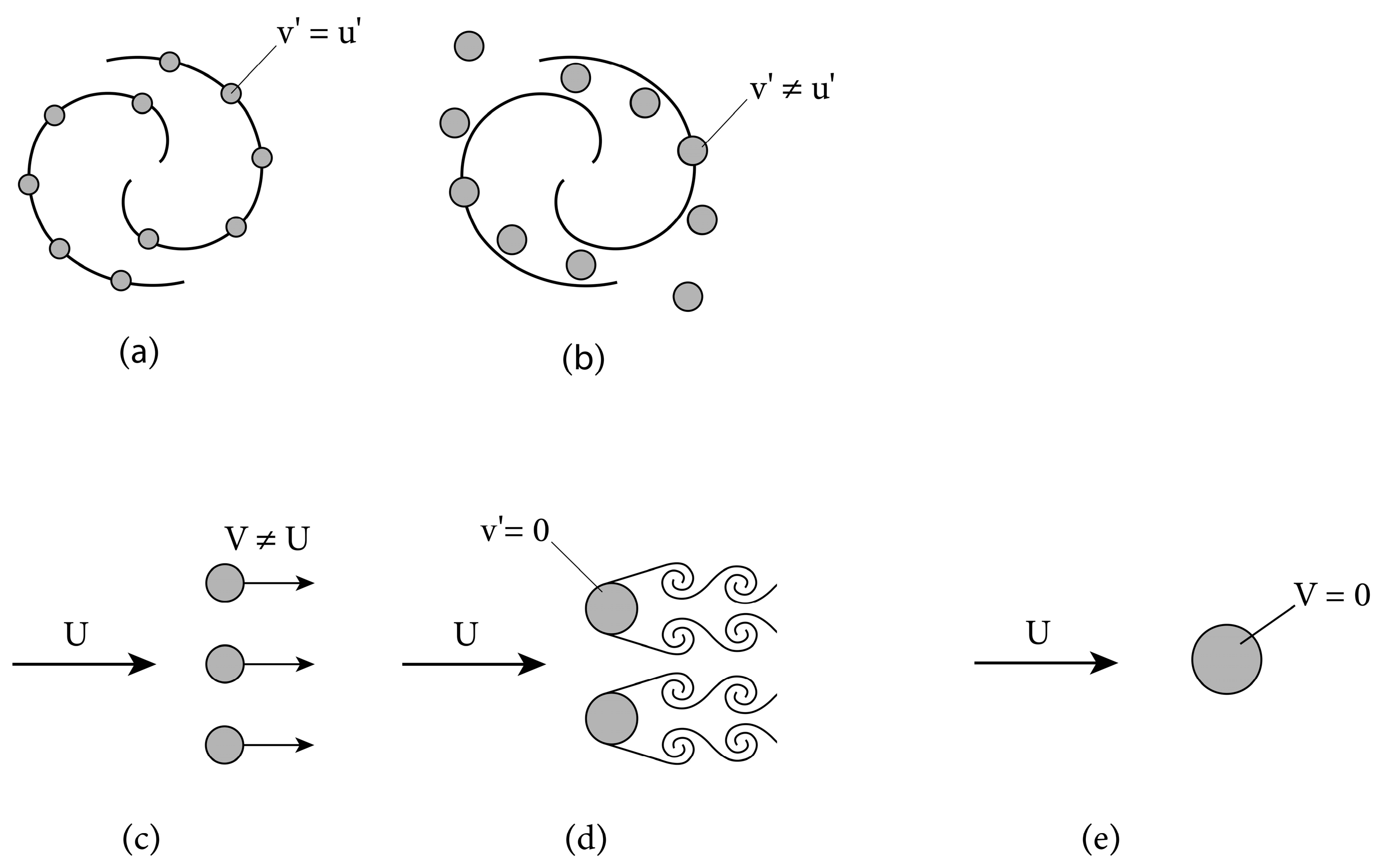
The development of mathematical modeling methods for two-phase flows with relatively large particles (non-equilibrium flows) that only interact with large energy-carrying vortices and are characterized by dynamic slippage (velocity difference) in relation to average motion.

(2)

The development of mathematical modeling methods for two-phase flows with large particles, which form turbulent wakes behind them. With the increase in particle concentration, these turbulent wakes will interfere with each other, and the particles will undergo collisions.

(3)

The development of mathematical modeling methods for two-phase flows containing particles of different sizes (polydisperse particles). Such flows are of interest to practicing engineers. Particles of different sizes will have different velocities and different effects on gas flow and tend to collide with each other at lower concentrations.

The development of mathematical modeling methods for two-phase flows with particles complicated by phase transitions (melting and subsequent evaporation) and chemical reactions (primarily combustion reactions).

References

1. Crowe, C.; Sommerfeld, M.; Tsuji, Y. (Eds.) Multiphase Flows with Droplets and Particles; CRC Press: Boca Raton, FL, USA, 1998; 471p. [Google Scholar]
2. Varaksin, A.Y. Turbulent Particle-Laden Gas Flows; Springer: New York, NY, USA, 2007; 210p. [Google Scholar]
3. Michaelides, E.E.; Crowe, C.T.; Schwarzkopf, J.D. (Eds.) Multiphase Flow Handbook, 2nd ed.; CRC Press: Boca Raton, FL, USA, 2017; 1396p. [Google Scholar]
4. Varaksin, A.Y.; Romash, M.E.; Kopeitsev, V.N. Tornado; Begell House: New York, NY, USA, 2015; 394p. [Google Scholar]
5. Elghobashi, S. Direct numerical simulation of turbulent flows laden with droplets of bubbles. Annu. Rev. Fluid Mech. 2019, 51, 217–244. [Google Scholar] [CrossRef] [Green Version]
6. Varaksin, A.Y. Collisions in Particle-Laden Gas Flows; Begell House: New York, NY, USA, 2013; 370p. [Google Scholar]
7. Varaksin, A.Y. Two-phase flows with solid particles, droplets, and bubbles: Problems and research results (review). High Temp. 2020, 58, 595–614. [Google Scholar] [CrossRef]
8. Elghobashi, S. Particle-laden turbulent flows. Appl. Sci. Res. 1991, 48, 301–314. [Google Scholar] [CrossRef]
9. Elghobashi, S. On predicting particle-laden turbulent flows. Appl. Sci. Res. 1994, 52, 309–329. [Google Scholar] [CrossRef]
10. Tsuji, Y.; Morikawa, Y. LDV Measurements of an air-solid two-phase flow in a horizontal pipe. J. Fluid Mech. 1982, 120, 385–409. [Google Scholar] [CrossRef]
11. Tsuji, Y.; Morikawa, Y.; Shiomi, H. LDV measurements of an air-solid two-phase flow in a vertical pipe. J. Fluid Mech. 1984, 139, 417–434. [Google Scholar] [CrossRef]
12. Rogers, C.B.; Eaton, J.K. The behavior of small particles in a vertical turbulent boundary layer in air. Int. J. Multiph. Flow 1990, 16, 819–834. [Google Scholar] [CrossRef]
13. Kulick, J.D.; Fessler, J.R.; Eaton, J.K. Particle response and turbulence modification in fully developed channel flow. J. Fluid Mech. 1994, 277, 109–134. [Google Scholar] [CrossRef]
14. Varaksin, A.Y.; Polezhaev, Y.V.; Polyakov, A.F. Effect of particle concentration on fluctuating velocity of the disperse phase for turbulent pipe flow. Int. J. Heat Fluid Flow 2000, 21, 562–567. [Google Scholar] [CrossRef]
15. Saffman, P.G.; Turner, J.S. On the collision of drops in turbulent cloud. J. Fluid Mech. 1956, 1, 16–30. [Google Scholar] [CrossRef] [Green Version]
16. Wang, L.-P.; Wexler, A.S.; Zhou, Y. On the collision rate of small particles in isotropic turbulence. I. Zero-inertia case. Phys. Fluids 1998, 10, 2647–2651. [Google Scholar] [CrossRef] [Green Version]
17. Wang, L.-P.; Wexler, A.S.; Zhou, Y. Statistical mechanical description and modelling of turbulent collision of inertial particles. J. Fluid Mech. 2000, 415, 117–153. [Google Scholar] [CrossRef] [Green Version]
18. Varaksin, A.Y. Collision of particles and droplets in turbulent two-phase flows. High Temp. 2019, 57, 555–572. [Google Scholar] [CrossRef]
19. Squires, K.D.; Eaton, J.K. Particle response and turbulence modification in isotropic turbulence. Phys. Fluids A 1990, 2, 1191–1203. [Google Scholar] [CrossRef]
20. Squires, K.D.; Eaton, J.K. Preferential concentration of particles by turbulence. Phys. Fluids A 1991, 3, 1169–1178. [Google Scholar] [CrossRef]
21. Fessler, J.R.; Kulick, J.D.; Eaton, J.K. Preferential concentration of heavy particles in a turbulent channel flow. Phys. Fluids 1994, 6, 3742–3749. [Google Scholar] [CrossRef]
22. Rouson, D.W.I.; Eaton, J.K. On the preferential concentration of solid particles in turbulent channel flow. J. Fluid Mech. 2001, 428, 149–169. [Google Scholar] [CrossRef]
23. Osiptsov, A.N. Investigation of regions of unbounded growth of the particle concentration in disperse flows. Fluid Dyn. 1984, 19, 378–385. [Google Scholar] [CrossRef]
24. Volkov, A.N.; Tsirkunov, Y.M.; Oesterle, B. Numerical simulation of a supersonic gas-solid flow over a blunt body: The role of inter-particle collisions and two-way coupling effects. Int. J. Multiph. Flow 2005, 31, 1244–1275. [Google Scholar] [CrossRef]
25. Varaksin, A.Y.; Romash, M.E.; Kopeitsev, V.N. Tornado-like gas-solid flow. AIP Conf. Proc. 2010, 1207, 342–347. [Google Scholar]
26. Varaksin, A.Y.; Romash, M.E.; Kopeitsev, V.N.; Gorbachev, M.A. Experimental study of wall-free non-stationary vortices generation due to air unstable stratification. Int. J. Heat Mass Transf. Transf. 2012, 55, 6567–6572. [Google Scholar] [CrossRef]
27. Varaksin, A.Y.; Romash, M.E.; Kopeitsev, V.N. Effect of net structures on wall-free non-stationary air heat vortices. Int. J. Heat Mass Transf. 2013, 64, 817–828. [Google Scholar] [CrossRef]
28. Varaksin, A.Y.; Ryzhkov, S.V. Turbulence in two-phase flows with macro-, micro- and nanoparticles: A review. Symmetry 2022, 14, 2433. [Google Scholar] [CrossRef]
29. Varaksin, A.Y.; Ryzhkov, S.V. Particle-laden and droplet-laden two-phase flows past bodies (a review). Symmetry 2023, 15, 388. [Google Scholar] [CrossRef]
30. Sommerfeld, M. Analysis of collision effects for turbulent gas-particle flow in a horizontal channel. Part, I. Particle transport. Int. J. Multiph. Flow 2003, 29, 675–828. [Google Scholar] [CrossRef]
31. Gavin, L.B.; Naumov, V.A.; Shor, V.V. Numerical investigation of a gas jet with heavy particles on the basis of a two-parameter model of turbulence. J. Appl. Mech. Tech. Phys. 1984, 25, 56–61. [Google Scholar] [CrossRef]
32. Kondrat‘ev, L.V. Modeling of two-phase flow on the stabilized section of a pipe. In Turbulent Two-Phase Flows and Experimental Techniques (pt. 2); Academy of Sciences of the Estonian SSR: Tallinn, Estonia, 1985; pp. 144–148. (In Russian) [Google Scholar]
33. Chen, C.P.; Wood, P.E. A turbulence closure model for dilute gas-particle flows. Can. J. Chem. Eng. 1985, 63, 349–360. [Google Scholar] [CrossRef]
34. Volkov, E.P.; Zaichik, L.I.; Pershukov, V.A. Simulation of the Combustion of Solid Fuels; Nauka: Moscow, Russian, 1994; 320p. (In Russian) [Google Scholar]
35. Melville, W.K.; Bray, K.N.C. A model of the two-phase turbulent jet. Int. J. Heat Mass Transf. 1979, 22, 647–656. [Google Scholar] [CrossRef]
36. Zaichik, L.I.; Alipchenkov, V.M.; Sinaiski, E.G. Particles in Turbulent Flows; Wiley-VCH: Darmstadt, Germany, 2008; 320p. [Google Scholar]
37. Buyevich, Y.A. Statistical hydrodynamics of disperse systems. Part 1. Physical background and general equations. J. Fluid Mech. 1971, 49, 489–507. [Google Scholar] [CrossRef]
38. Derevich, I.V.; Zaichik, L.I. Particle deposition from a turbulent flow. Fluid Dyn. 1988, 23, 722–729. [Google Scholar] [CrossRef]
39. Derevich, I.V.; Zaichik, L.I. An equation for the probability density velocity and temperature of particles in a turbulent flow modeled by a random Gaussian field. J. Appl. Math. Mech. 1990, 54, 631–636. [Google Scholar] [CrossRef]
40. Zaichik, L.I. Models of turbulent momentum and heat transfer in a dispersed phase based on equations for the second and third moments of particle velocity and temperature fluctuations. J. Eng. Phys. Thermophys. 1992, 63, 976–984. [Google Scholar] [CrossRef]
41. Zaichik, L.I. Modelling of the motion of particles in non-uniform turbulent flow using the equation for the probability density function. J. Appl. Math. Mech. 1997, 61, 127–133. [Google Scholar] [CrossRef]
42. Swailes, D.C.; Darbyshire, K.F.F. A generalized Fokker-Plank equation for particle transport in random media. Physica A 1997, 242, 38–48. [Google Scholar] [CrossRef]
43. Hyland, K.E.; McKee, S.; Reeks, M.W. Derivation of a PDF kinetic equation for the transport of particles in turbulent flows. J. Phys. A Math. Gen. 1999, 32, 6169–6190. [Google Scholar] [CrossRef]
44. Zaichik, L.I. A statistical model of particle transport and heat transfer in turbulent shear flows. Phys. Fluids 1999, 11, 1521–1534. [Google Scholar] [CrossRef]
45. Derevich, I.V. Statistical modelling of mass transfer in turbulent two-phase dispersed flows. 1. Model development. Int. J. Heat Mass Transf. 2000, 43, 3709–3723. [Google Scholar] [CrossRef]
46. Pandya, R.V.R.; Mashayek, F. Kinetic equation for particle transport and heat transport in non-isothermal turbulent flows. AIAA Paper 2002, 41, 841–847. [Google Scholar] [CrossRef]
47. Zaichik, L.I.; Oesterle, B.; Alipchenkov, V.M. On the probability density function model for the transport of particles in anisotropic turbulent flow. Phys. Fluids 2004, 16, 1956–1964. [Google Scholar] [CrossRef]
48. Reeks, M.W. On a kinetic equation for the transport of particles in turbulent flows. Phys. Fluids A 1991, 3, 446–456. [Google Scholar] [CrossRef]
49. Reeks, M.W. On the continuum equation for dispersed particles in nonuniform flows. Phys. Fluids A 1992, 4, 1290–1303. [Google Scholar] [CrossRef]
50. Pandya, R.V.R.; Mashayek, F. Non-isotermal dispersed phase of particles in turbulent flow. J. Fluids Mech. 2003, 475, 205–245. [Google Scholar] [CrossRef]
51. Pozorski, J. Derivation of the kinetic equation for dispersed particles in turbulent flows. J. Theor. Appl. Mech. 1998, 36, 31–46. [Google Scholar]
52. Pozorski, J.; Minier, J.-P. Probability density function modeling of dispersed two-phase turbulent flows. Phys. Rev. E 1999, 59, 855–863. [Google Scholar] [CrossRef]
53. Pialat, X.; Simonin, O.; Villedieu, P. Direct coupling between Lagrangian and Eulerian approaches in turbulent gas-solid flows. In Proceedings of the ASME 2005 Fluids Engineering Division Summer Meeting, Houston, TX, USA, 19–23 June 2005. FEDS2006-98122. [Google Scholar]
54. Jones, W. Models for turbulent flows with variable density and combustion. In Prediction Methods for Turbulent Flows; Hemisphere: Washington, DC, USA, 1980; 468p. [Google Scholar]
55. Derevich, I.V.; Yeroshenko, V.M.; Zaichik, L.I. Hydrodynamics and heat transfer of turbulent gas suspension flows in tubes. 1. Hydrodynamics. Int. J. Heat Mass Transf. 1989, 32, 2329–2339. [Google Scholar] [CrossRef]
56. Derevich, I.V.; Yeroshenko, V.M.; Zaichik, L.I. Hydrodynamics and heat transfer of turbulent gas suspension flows in tubes. 2. Heat Transfer. Int. J. Heat Mass Transf. 1989, 32, 2341–2350. [Google Scholar] [CrossRef]
57. Abramovich, G.N. The effect of solid particle or drop addition on the structure of a turbulent gas jet. Dokl. Akad. Nauk SSSR 1970, 190, 1052–1055. (In Russian) [Google Scholar]
58. Abramovich, G.N.; Girshovich, T.A.; Krasheninnikov, S.Y.; Sekundov, A.N.; Smirnova, I.P. The Theory of Turbulent Jets; Nauka: Moscow, Russian, 1984; 717p. (In Russian) [Google Scholar]
59. Varaksin, A.Y. Effect of particles on carrier gas flow turbulence. High Temp. 2015, 53, 423–444. [Google Scholar] [CrossRef]
60. Eaton, J.K.; Fessler, J.R. Preferential concentration of particles by turbulence. Int. J. Multiph. Flow 1994, 20, 169–209. [Google Scholar] [CrossRef]
61. Fessler, J.R.; Eaton, J.K. Particle response in a planar sudden expansion flow. Exp. Therm. Fluid Sci. 1997, 15, 413–423. [Google Scholar] [CrossRef]
62. Fessler, J.R.; Eaton, J.K. Turbulence modification by particles in a backward-facing step flow. J. Fluid Mech. 1999, 394, 97–117. [Google Scholar] [CrossRef]
63. Yuan, Z.; Michaelides, E.E. Turbulence modulation in particulate flows–a theoretical approarch. Int. J. Multiph. Flow 1992, 18, 779–785. [Google Scholar] [CrossRef]
64. Yarin, L.P.; Hetsroni, G. Turbulence intensity in dilute two-phase flows–3. The particles-turbulence interaction in dilute two-phase flow. Int. J. Multiph. Flow 1994, 20, 27–44. [Google Scholar] [CrossRef]
65. Zaichik, L.I.; Varaksin, A.Y. Effect of the wake behind large particles on the turbulence intensity of carrier flow. High Temp. 1999, 37, 655–658. [Google Scholar]
66. Elghobashi, S.E.; Abou-Arab, T.W. A two-equation turbulence model for two-phase flows. Phys. Fluids 1983, 26, 931–938. [Google Scholar] [CrossRef]
67. Rizk, M.A.; Elghobashi, S.E. A two-equation turbulence model for dispersed dilute confined two-phase flows. Int. J. Multiph. Flow 1989, 15, 119–134. [Google Scholar] [CrossRef]
68. Mostafa, A.A.; Mongia, H.C. On the interaction of particles and turbulent fluid flow. Int. J. Heat Mass Transf. 1988, 31, 2063–2075. [Google Scholar] [CrossRef]
69. Berlemont, A.; Grancher, M.-S.; Gousbet, G. On the Lagrangian simulation of turbulence influence on droplet evaporation. Int. J. Heat Mass Transf. 1991, 34, 2805–2812. [Google Scholar] [CrossRef]
70. Burton, T.M.; Eaton, J. Fully resolved simulations of particle-turbulence interaction. J. Fluid Mech. 2005, 545, 67–111. [Google Scholar] [CrossRef]
71. Picano, F.; Breugem, W.P.; Brandt, L. Turbulent channel flow of dense suspensions of neutrally-buoyant spheres. J. Fluid Mech. 2015, 764, 463–487. [Google Scholar] [CrossRef] [Green Version]
72. ten Cate, A.; Derksen, J.J.; Portela, L.M.; van den Akker, H.E.A. Fully resolved simulations of colliding monodisperse spheres in forced isotropic turbulence. J. Fluid Mech. 2004, 539, 233–271. [Google Scholar] [CrossRef] [Green Version]
73. Takagi, S.; Oguz, H.N.; Zhang, Z.; Prosperetti, A. Physalis: A new method for particle simulation: Part ii: Two-dimensional Navier-Stokes flow around cylinders. J. Comput. Phys. 2003, 187, 371–390. [Google Scholar] [CrossRef]
74. Riley, J.J.; Patterson Jr, G.S. Diffusion experiments with numerically integrated isotropic turbulence. Phys. Fluids 1974, 17, 292–297. [Google Scholar] [CrossRef]
75. Yeung, P.K.; Pope, S.B. An algorithm for tracking fluid particles in numerical simulation of homogeneous turbulence. J. Comput. Phys. 1988, 79, 373–416. [Google Scholar] [CrossRef]
76. Balachandar, S.; Maxey, M.R. Methods for evaluating fluid velocities in spectral simulations of turbulence. J. Comput. Phys. 1989, 83, 96–125. [Google Scholar] [CrossRef]
77. McLaughlin, J.B. Aerosol particle deposition in numerically simulated channel flow. Phys. Fluids 1989, A1, 1211–1224. [Google Scholar] [CrossRef]
78. Kontomaris, K.; Hanratty, T.J.; McLaughlin, J.B. An algorithm for tracking fluid particles in a spectral simulation of turbulent channel flow. J. Comput. Phys. 1992, 103, 231–242. [Google Scholar] [CrossRef]
79. Marchioli, C.; Soldati, A.; Kuerten, J.G.M.; Arcen, B.; Taniere, A.; Goldensoph, G.; Squires, K.D.; Cargnelutti, M.F.; Portela, L.M. Statistics of particle dispersion in direct numerical simulations of wallbounded turbulence: Results of an international collaborative benchmark test. Int. J. Multiph. Flow 2008, 34, 879–893. [Google Scholar] [CrossRef] [Green Version]
80. Marchioli, C.; Giusti, A.; Salvetti, M.V.; Soldati, A. Direct numerical simulation of particle wall transfer and deposition in upward turbulent pipe flow. Int. J. Multiph. Flow 2003, 29, 1017–1038. [Google Scholar] [CrossRef]
81. van Esch, B.P.M.; Kuerten, J.G.M. Direct numerical simulation of the motion of particles in rotating pipe flow. J. Turbul. 2008, 9, N4. [Google Scholar] [CrossRef]
82. Picano, F.; Sardina, G.; Casciola, C.M. Spatial development of particle-laden turbulent pipe flow. Phys. Fluids 2009, 21, 093305. [Google Scholar] [CrossRef]
83. Elghobashi, S.; Truesdell, G.C. Direct simulation of particle dispersion in a decaying isotropic turbulence. J. Fluid Mech. 1992, 242, 655–700. [Google Scholar] [CrossRef]
84. Boivin, M.; Simonin, O.; Squires, K.D. Direct numerical simulation of turbulence modulation by particles in homogeneous turbulence. J. Fluid Mech. 1998, 375, 235–263. [Google Scholar] [CrossRef] [Green Version]
85. Eaton, J.K. Two-way coupled turbulence simulations of gas-particle flows using point-particle tracking. Int. J. Multiph. Flow 2009, 35, 792–800. [Google Scholar] [CrossRef]
86. Kuerten, J.G.M.; Vreman, A.W. Effect of droplet interaction on droplet-laden turbulent channel flow. Phys. Fluids 2015, 27, 053304. [Google Scholar] [CrossRef] [Green Version]
87. Russo, E.; Kuerten, J.G.M.; van der Geld, C.W.M.; Geurts, B.J. Water droplet condensation and evaporation in turbulent channel flow. J. Fluid Mech. 2014, 749, 666–700. [Google Scholar] [CrossRef]
88. Pan, Y.; Banerjee, S. Numerical simulation of particle interactions with wall turbulence. Phys. Fluids 1996, 8, 2733–2755. [Google Scholar] [CrossRef]
89. Zhao, L.H.; Andersson, H.I.; Gillissen, J.J.J. Turbulence modulation and drag reduction by spherical particles. Phys. Fluids 2010, 22, 081702. [Google Scholar] [CrossRef] [Green Version]
90. Zhao, L.H.; Andersson, H.I.; Gillissen, J.J.J. Interphasial energy transfer and particle dissipation in particle-laden wall turbulence. J. Fluid Mech. 2013, 715, 32–59. [Google Scholar] [CrossRef] [Green Version]
91. Lee, J.; Lee, C. Modification of particle-laden near-wall turbulence; effect of Stokes number. Phys. Fluids 2015, 27, 023303. [Google Scholar] [CrossRef] [Green Version]
92. Letournel, R.; Laurent, F.; Massot, M.; Vie, A. Modulation of homogeneous and isotropic turbulence by sub-Kolmogorov particles: Impact of particle field heterogeneity. Int. J. Multiph. Flow 2020, 125, 103233. [Google Scholar] [CrossRef]
93. Yu, Z.; Xia, Y.; Lin, J. Modulation of turbulence intensity by heavy finite-size particles in upward channel flow. J. Fluid Mech. 2021, 913, A3. [Google Scholar] [CrossRef]
94. Vreman, A.W. Turbulence characteristics of particle-laden pipe flow. J. Fluid Mech. 2007, 584, 235–279. [Google Scholar] [CrossRef]
95. Vreman, A.W. Turbulence attenuation in particle-laden flow in smooth and rough channels. J. Fluid Mech. 2015, 773, 103–136. [Google Scholar] [CrossRef] [Green Version]
96. Mallouppas, G.; George, W.K.; van Wachem, B.G.M. Dissipation and inter-scale transfer in fully coupled particle and fluid motions in homogeneous isotropic forced turbulence. Int. J. Heat Fluid Flow 2017, 67, 74–85. [Google Scholar] [CrossRef] [Green Version]
97. Smagorinsky, J. General circulation experiments with the primitive equations. Mon. Weather Rev. 1963, 91, 99–164. [Google Scholar] [CrossRef]
98. Bardina, J.; Ferziger, J.H.; Reynolds, W.C. Improved Turbulence Models Based on LES of Homogeneous Incompressible Turbulent Flows; Technical Report No. TF-19; Stanford, Depart. Mech. Eng.: Stanford, CA, USA, 1984. [Google Scholar]
99. Clark, R.A.; Ferziger, J.H.; Reynolds, W.C. Evaluation of subgrid-scale models using an accurately simulated turbulent flow. J. Fluid Mech. 1979, 91, 1–16. [Google Scholar] [CrossRef]
100. Stolz, S.; Adams, N.A.; Kleiser, L. An approximate deconvolution model for large-eddy simulation with application to incompressible wall-bounded flows. Phys. Fluids 2001, 13, 997–1015. [Google Scholar] [CrossRef]
101. Deardorff, J.W.; Peskin, R.L. Lagrangian statistics from numerically integrated turbulent shear flow. Phys. Fluids 1970, 13, 584–595. [Google Scholar] [CrossRef]
102. Uijttewaal, W.S.J.; Oliemans, R.V.A. Particle dispersion and deposition in direct numerical and large eddy simulation of vertical pipe flows. Phys. Fluids 1996, 8, 2590–2604. [Google Scholar] [CrossRef]
103. Wang, Q.; Squires, K.D. Large eddy simulation of particle deposition in a vertical turbulent channel flow. Int. J. Multiph. Flow 1996, 22, 667–683. [Google Scholar] [CrossRef]
104. Germano, M.; Piomelli, U.; Moin, P.; Cabot, W.H. A dynamic subgrid-scale eddy viscosity model. Phys. Fluids 1991, A3, 1760–1765. [Google Scholar] [CrossRef]
105. Boivin, M.; Simonin, O.; Squires, K.D. On the prediction of gas-solid flows with two-way coupling using large eddy simulation. Phys. Fluids 2000, 12, 2080–2090. [Google Scholar] [CrossRef] [Green Version]
106. Yamamoto, Y.; Potthoff, M.; Tanaka, T.; Kajishima, T.; Tsuji, Y. Large-eddy simulation of turbulent gas-particle flow in a vertical channel: Effect of considering inter-particle collisions. J. Fluid Mech. 2001, 442, 303–334. [Google Scholar] [CrossRef] [Green Version]
107. Vreman, A.W.; Geurts, B.J.; Deen, N.G.; Kuipers, J.A.M.; Kuerten, J.G.M. Two- and four-way coupled Euler-Lagrangian large-eddy simulation of turbulent particle-laden channel flow. Flow Turbul. Combust. 2009, 82, 47–71. [Google Scholar] [CrossRef] [Green Version]
108. Mallouppas, G.; van Wachem, B. Large eddy simulations of turbulent particle-laden channel flow. Int. J. Multiph. Flow 2013, 54, 65–75. [Google Scholar] [CrossRef] [Green Version]
109. Breuer, M.; Alletto, M. Efficient simulation of particle-laden turbulent flows with high mass loadings using LES. Int. J. Heat Fluid Flow 2012, 35, 2–12. [Google Scholar] [CrossRef]
110. Pozorski, J.; Apte, S.V. Filtered particle tracking in isotropic turbulence and stochastic modeling of subgrid-scale dispersion. Int. J. Multiph. Flow 2009, 35, 118–128. [Google Scholar] [CrossRef]
111. Alletto, M.; Breuer, M. Prediction of turbulent particle-laden flow in horizontal smooth and rough pipes inducing secondary flow. Int. J. Multiph. flow 2013, 55, 80–98. [Google Scholar] [CrossRef]
112. Breuer, M.; Almohammed, N. Modeling and simulation of particle agglomeration in turbulent flows using a hard-sphere model with deterministic collision detection and enhanced structure models. Int. J. Multiph. Flow 2015, 73, 171–206. [Google Scholar] [CrossRef]
113. Kuzenov, V.V.; Ryzhkov, S.V. Approximate calculation of convective heat transfer near hypersonic aircraft surface. J. Enhanc. Heat Transf. 2018, 25, 181–193. [Google Scholar] [CrossRef]
114. Kuzenov, V.V.; Ryzhkov, S.V. The Qualitative and Quantitative Study of Radiation Sources with a Model Configuration of the Electrode System. Symmetry 2021, 13, 927. [Google Scholar] [CrossRef]
115. Kuzenov, V.V.; Ryzhkov, S.V. Estimation of the neutron generation in the combined magneto-inertial fusion scheme. Phys. Scr. 2021, 96, 125613. [Google Scholar] [CrossRef]
116. Kuzenov, V.V.; Ryzhkov, S.V. Numerical Simulation of Pulsed Jets of a High-Current Pulsed Surface Discharge. Comput. Therm. Sci. 2021, 13, 45–56. [Google Scholar] [CrossRef]
117. Kuzenov, V.V.; Ryzhkov, S.V.; Varaksin, A.Y. Calculation of heat transfer and drag coefficients for aircraft geometric models. Appl. Sci. 2022, 12, 11011. [Google Scholar] [CrossRef]
118. Kuzenov, V.V.; Ryzhkov, S.V.; Frolko, P.A. Numerical simulation of the coaxial magneto-plasma accelerator and non-axisymmetric radio frequency discharge. J. Phys. Conf. Ser. 2017, 830, 012049. [Google Scholar] [CrossRef]
119. Kuzenov, V.V.; Ryzhkov, S.V.; Varaksin, A.Y. The Adaptive Composite Block-Structured Grid Calculation of the Gas-Dynamic Characteristics of an Aircraft Moving in a Gas Environment. Mathematics 2022, 10, 2130. [Google Scholar] [CrossRef]
120. Engler, M.; Kockmann, N.; Kiefer, T.; Woias, P. Numerical and experimental investigations on liquid mixing in static micromixers. Chem. Eng. J. 2004, 101, 315. [Google Scholar] [CrossRef]
121. Lobasov, A.; Minakov, A. Analyzing mixing quality in a T-shaped micromixer for different fluids properties through numerical simulation. Chem. Eng. Process 2018, 124, 11. [Google Scholar] [CrossRef] [Green Version]
122. Mariotti, A.; Galletti, C.; Brunazzi, E.; Salvetti, M.V. Unsteady flow regimes in arrow-shaped micro-mixers with different tilting angles. Phys. Fluids 2021, 33, 012008. [Google Scholar] [CrossRef]
Figure 1. Classification of turbulent two-phase flows’ dependence on particle inertia.
Mathematics 11 03290 g001
Figure 2. Simplified schemes of turbulent two-phase flows of different classes depending on particle inertia: (a) equilibrium flow, (b) quasi-equilibrium flow, (c) nonequilibrium flow, (d) flow with large particles, (e) and flow around fixed “frozen” particles.
Mathematics 11 03290 g002
Figure 3. Classification of approaches to numerical simulation of two-phase flows depending on different levels of turbulence description and interphase coupling.
Mathematics 11 03290 g003
Disclaimer/Publisher’s Note: The statements, opinions and data contained in all publications are solely those of the individual author(s) and contributor(s) and not of MDPI and/or the editor(s). MDPI and/or the editor(s) disclaim responsibility for any injury to people or property resulting from any ideas, methods, instructions or products referred to in the content.