
Eulerian-Eulerian Modeling of the Features of Mean and Fluctuational Flow Structure and Dispersed Phase Motion in Axisymmetric Round Two-Phase Jets

Abstract
:1. Introduction
2. Mathematical Model
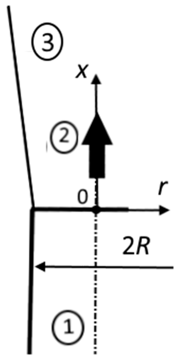
2.1. Bubbly Free Round Jet
2.1.1. Carrier Phase (Liquid)
2.1.2. Dispersed Phase (Gas Bubbles)
2.2. Gas-Droplet Jet
2.2.1. Carrier Phase (Gas)
2.2.2. Dispersed Phase (Liquid Droplets)
2.3. SMC Model of Carrier Phase Turbulence for Bubbly and Gas-Droplet Flows
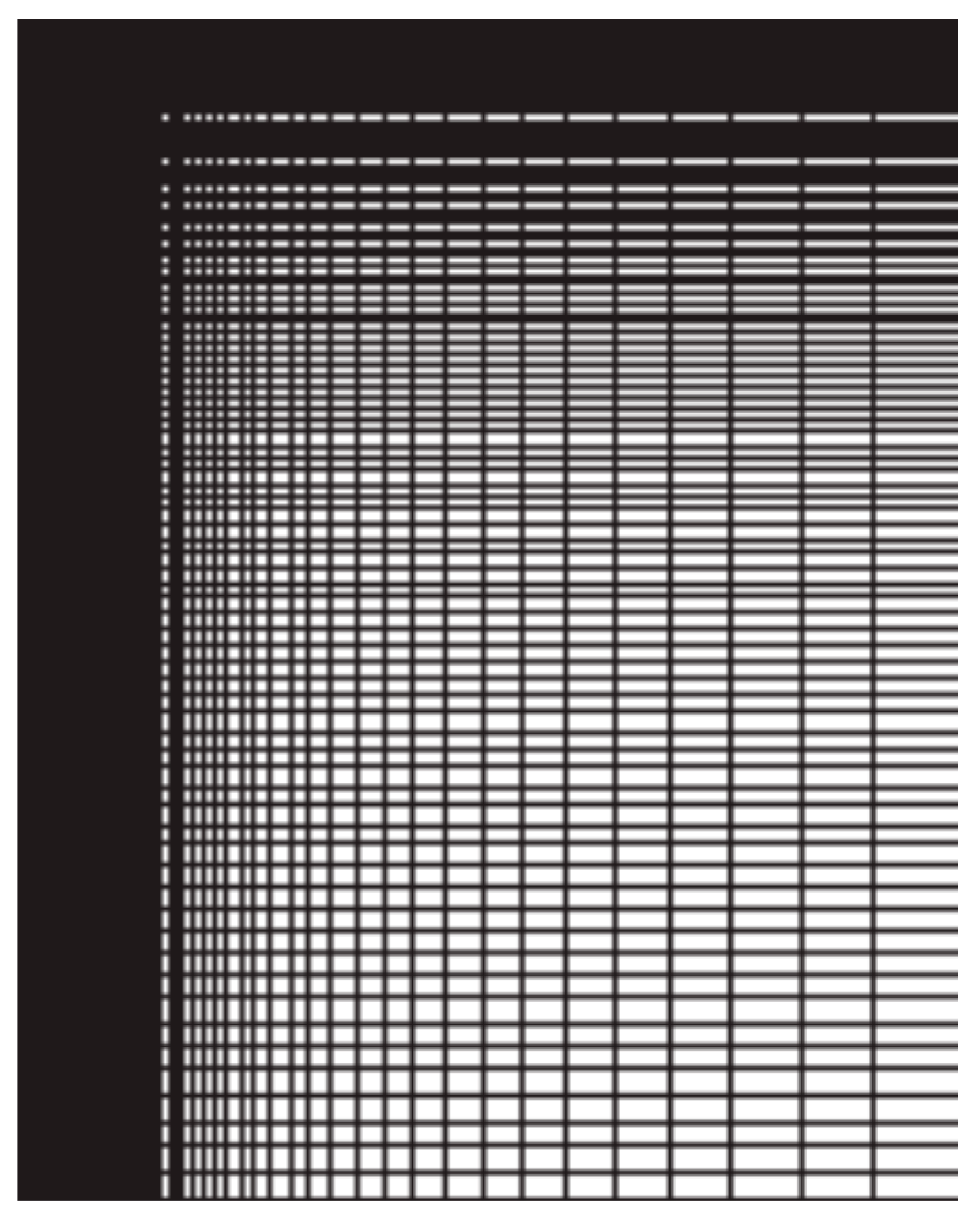
3. Numerical Implementation
4. Comparison with Data from Other Works
4.1. Comparisons with Measurement Results for a Single-Phase Gas Jet
4.2. Comparison with Measurement Data for Two-Phase Submerged Gas-Dispersed, Gas-Droplet and Bubbly Jets
5. The Results of Numerical Simulation and Analysis
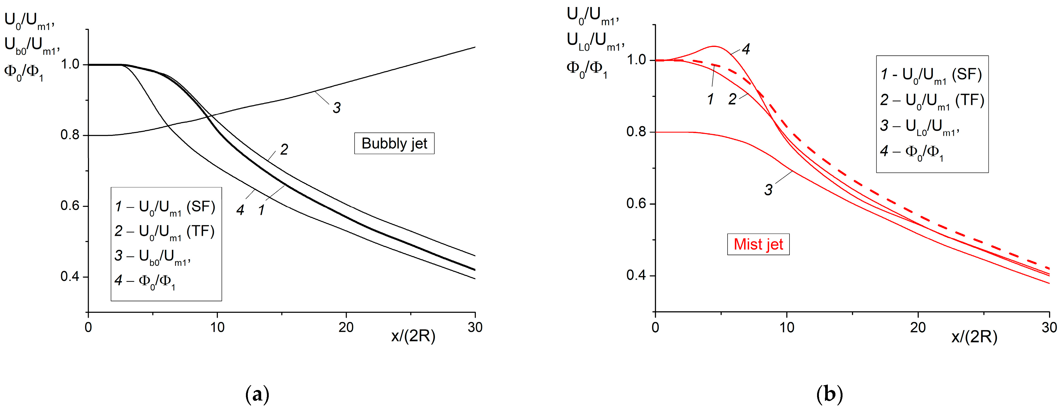
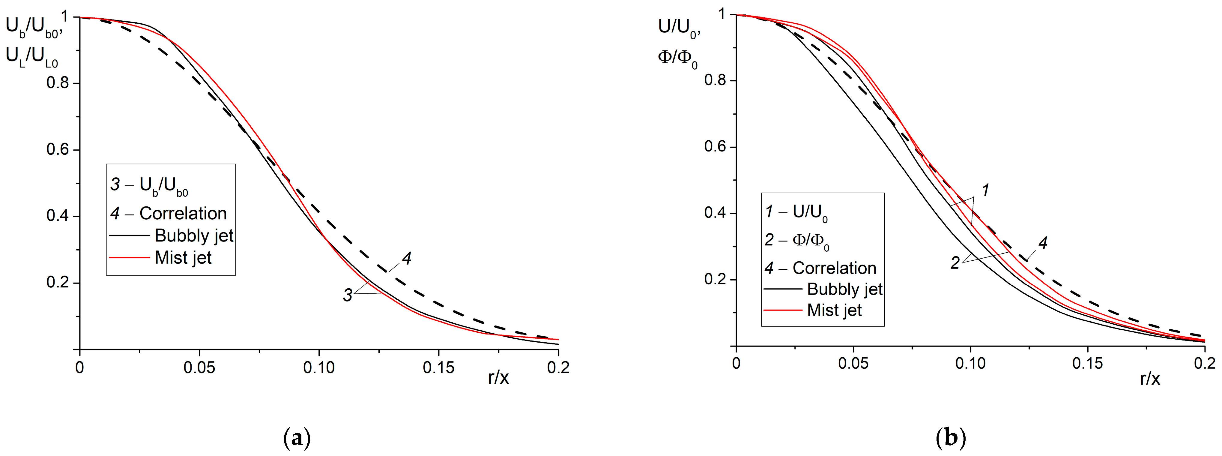
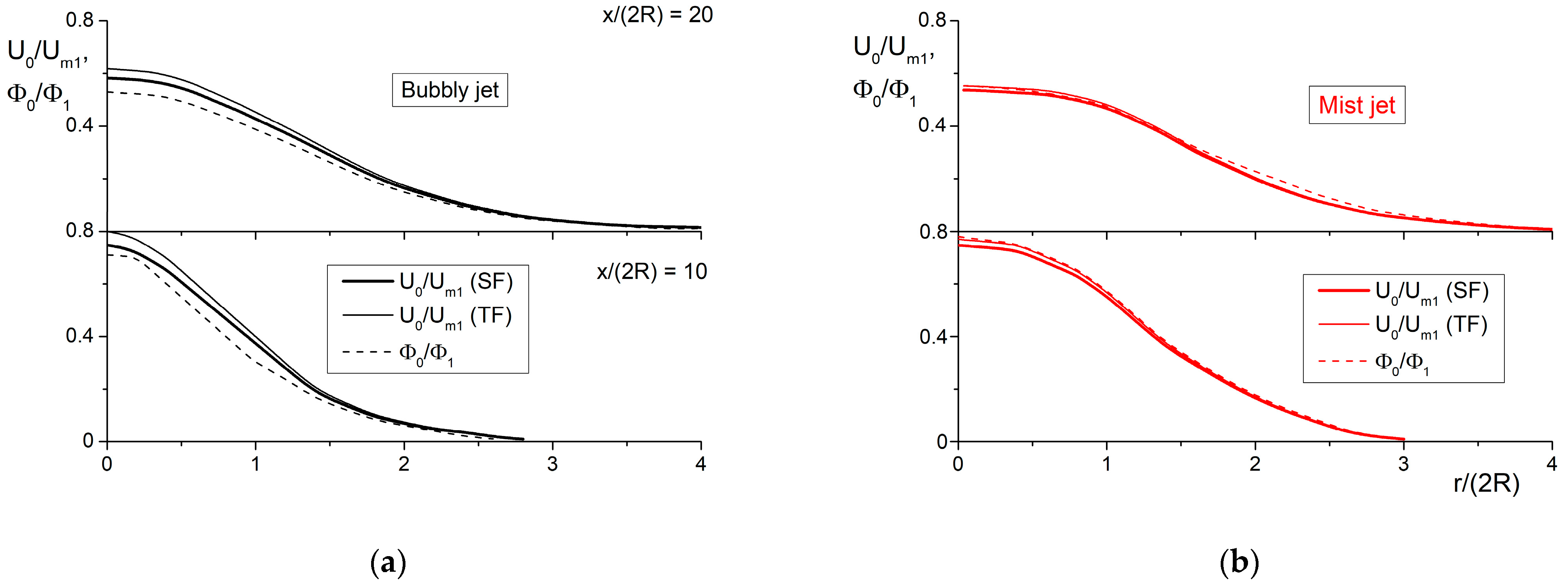
5.1. Flow Structure
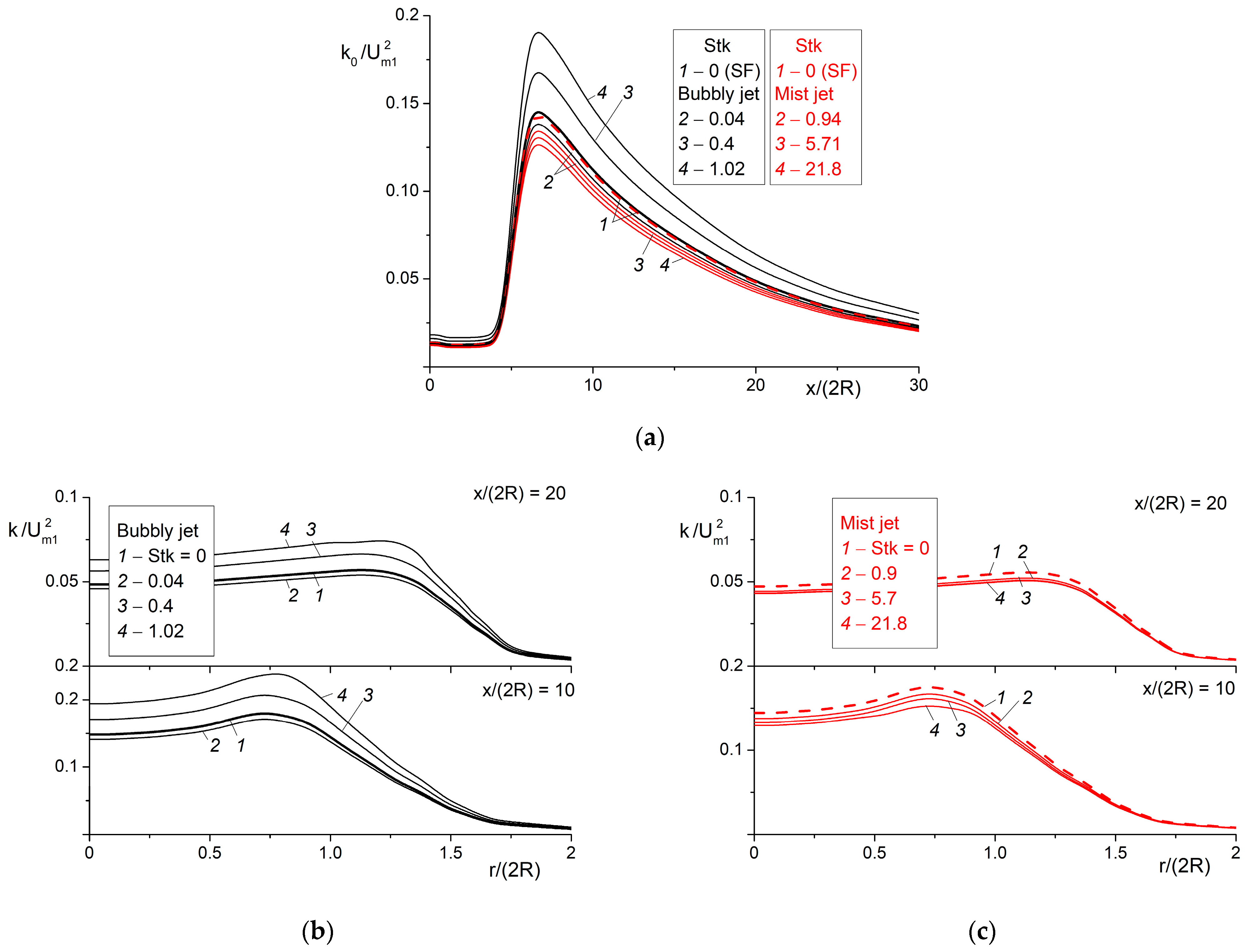
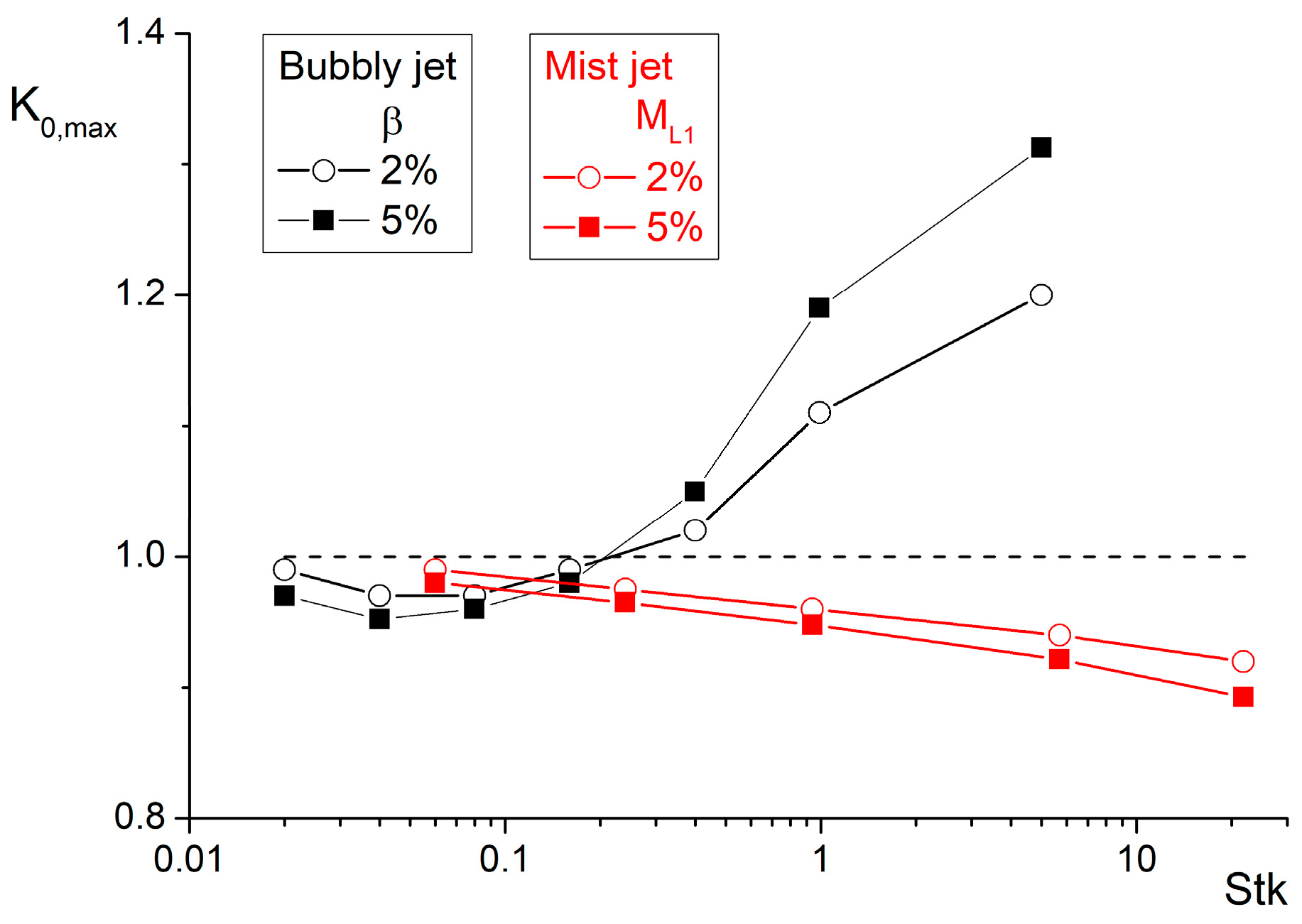
5.2. Turbulence
6. Comparison with Experimental Data for a Gas-Droplet Jet with Evaporating Droplets
7. Conclusions
8. Unresolved Problems
Author Contributions
Funding
Data Availability Statement
Conflicts of Interest
Nomenclature
| d | bubble or droplet diameter |
| turbulent kinetic energy | |
| ML | mass fraction |
| m | mass of all particles (bubbles or droplets) |
| N | numerical concentrations |
| 2R | pipe outlet diameter |
| Re = Um12R/ν | Reynolds number |
| Reynolds number | |
| Stk = τ/τf | the average Stokes number |
| UL | the droplet velocity (vector) |
| Um1 | mean-mass average flow velocity |
| US | the carrier fluid velocity seen by the bubble or droplet (vector) |
| u* | wall friction velocity |
| x | streamwise coordinate |
| y | distance normal from the wall |
| Subscripts | |
| 0 | jet axis |
| 1 | initial condition |
| W | wall |
| b | bubble |
| l | liquid |
| m | mean-mass |
| Greek | |
| Φ | volume fraction |
| β | gas volumetric flow rate ratio |
| ε | dissipation of the turbulent kinetic energy |
| μ | dynamic viscosity |
| ν | kinematic viscosity |
| ρ | density |
| τ | droplet relaxation time |
| τV | viscous stress |
| τW | wall shear stress |
| Acronym | |
| CV | control volume |
| EE | Eulerian-Eulerian |
| EA | Eulerian-Lagrangian |
| KET | kinetic energy of turbulence |
| RANS | Reynolds-averaged Navier-Stokes |
| SMC | second moment closure |
| SF | single-phase flow |
| TF | two-phase flow |
References
- Nigmatulin, R.I. Dynamics of Multiphase Media; V. 1; Hemisphere: New York, NY, USA, 1991. [Google Scholar]
- Ishii, M.; Hibiki, T. Thermo-Fluid Dynamics of Two-Phase Flow; Springer: Berlin, Germany, 2011. [Google Scholar]
- Sirignano, W.A. Fluid Dynamics and Transport of Droplets and Sprays; Cambridge University Press: Cambridge, UK, 1999. [Google Scholar]
- Jenny, P.; Roekaerts, D.; Beishuizen, N. Modeling of turbulent dilute spray combustion. Progr. Energy Combust. Sci. 2012, 38, 846–887. [Google Scholar] [CrossRef]
- Reeks, M.W. On a kinetic equation for the transport of particles in turbulent flows. Phys. Fluids A 1991, 3, 446–456. [Google Scholar] [CrossRef]
- Sun, T.Y.; Faeth, G.M. Structure of turbulent bubbly jets—I: Methods and centerline properties. Int. J. Multiph. Flow 1986, 12, 99–114. [Google Scholar] [CrossRef]
- Abramovich, G.N. On the influence of solid particles or drops on the structure of a turbulent gas jet. Dokl. USSR 1970, 190, 1052–1055. (In Russian) [Google Scholar]
- Laats, M.K.; Frishman, F.A. Assumptions used in calculating the two-phase jet. Fluid Dyn. 1970, 5, 333–338. [Google Scholar] [CrossRef]
- Zuev, Y.V.; Lepeshinskii, I.A. Mathematical model of a two-phase turbulent jet. Fluid Dyn. 1981, 16, 857–864. [Google Scholar] [CrossRef]
- Kartushinskii, A.I. Explanation of the anomalous dispersal of the discrete particles in a two-phase turbulent jet with allowance for their inertia. Fluid Dyn. 1984, 19, 29–34. [Google Scholar] [CrossRef]
- Shearer, A.J.; Tamura, H.; Faeth, G.M. Evaluation of a locally homogeneous flow model of spray evaporation. J. Energy 1979, 3, 271–278. [Google Scholar] [CrossRef]
- Vinberg, A.A.; Zaichik, L.I.; Pershukov, V.A. Computational model of turbulent gas-disperse jet flows. J. Eng. Phys. 1991, 61, 1199–1206. [Google Scholar] [CrossRef]
- Solomon, A.S.P.; Shuen, J.S.; Zhang, Q.F.; Faeth, G.M. Measurements and predictions of the structure of evaporating sprays. ASME J. Heat Transf. 1985, 107, 679–686. [Google Scholar] [CrossRef]
- Mostafa, A.A.; Mongia, H.C. On the modeling of turbulent evaporating sprays: Eulerian versus Lagrangian approach. Int. J. Heat Mass Transf. 1987, 30, 2583–2593. [Google Scholar] [CrossRef]
- Zuev, Y.V.; Lepeshinsky, I.A. Two-phase multicomponent turbulent jet with phase transitions. Fluid Dyn. 1995, 30, 750–757. [Google Scholar] [CrossRef]
- Sommerfeld, M. Analysis of isothermal and evaporating turbulent sprays by phase-doppler anemometry and numerical calculations. Int. J. Heat Fluid Flow 1998, 19, 173–186. [Google Scholar] [CrossRef]
- Prevost, F.; Boree, J.; Nuglish, H.J.; Sharnay, G. Measurements of fluid/particle correlated motion in the far field of an axisymmetric jet. Int. J. Multiph. Flow 1996, 22, 686–701. [Google Scholar] [CrossRef]
- Amani, E.; Nobari, M.R.H. Systematic tuning of dispersion models for simulation of evaporating sprays. Int. J. Multiph. Flow 2013, 48, 11–31. [Google Scholar] [CrossRef]
- Alekseenko, S.V.; Anufriev, I.S.; Dekterev, A.A.; Kuznetsov, V.A.; Maltsev, L.I.; Minakov, A.V.; Chernetskiy, M.Y.; Shadrin, E.Y.; Sharypov, O.V. Experimental and numerical investigation of aerodynamics of a pneumatic nozzle for suspension fuel. Int. J. Heat Fluid Flow 2019, 77, 288–298. [Google Scholar] [CrossRef]
- Sun, T.Y.; Faeth, G.M. Structure of turbulent bubbly jets—II: Phase properties and profiles. Int. J. Multiph. Flow 1986, 12, 115–126. [Google Scholar] [CrossRef]
- Iguchi, M.; Okita, K.; Nakatani, T.; Kasai, N. Structure of turbulent round bubbling jet generated by premixed gas and liquid injection. Int. J. Multiph. Flow. 1997, 23, 249–262. [Google Scholar] [CrossRef]
- Lopez de Bertodano, M.; Moraga, F.J.; Drew, D.A.; Lahey, R.T., Jr. The modeling of lift and dispersion forces in two-fluid model simulations of a bubbly jet. ASME J. Fluids Eng. 2004, 126, 573–580. [Google Scholar] [CrossRef]
- Alekseenko, S.V.; Dulin, V.M.; Markovich, D.M.; Pervunin, K.S. Experimental investigation of turbulence modification in bubbly axisymmetric jets. J. Eng. Thermophys. 2015, 24, 101–112. [Google Scholar] [CrossRef]
- Poletaev, I.; Tokarev, M.P.; Pervunin, K.S. Bubble patterns recognition using neural networks: Application to the analysis of a two-phase bubbly jet. Int. J. Multiph. Flow 2020, 126, 103194. [Google Scholar] [CrossRef]
- Seo, H.; Kim, K.C. Experimental study on flow and turbulence characteristics of bubbly jet with low void fraction. Int. J. Multiph. Flow 2021, 142, 103748. [Google Scholar] [CrossRef]
- Kuo, T.W.; Bracco, F.V. On the scaling of impulsively started incompressible turbulent round jet. ASME J. Fluids Eng. 1982, 104, 191–197. [Google Scholar] [CrossRef]
- Sanjose, M.; Senoner, J.M.; Jaegle, F.; Cuenot, B.; Moreau, S.; Poinsot, T. Fuel injection model for Euler–Euler and Euler–Lagrange large-eddy simulations of an evaporating spray inside an aeronautical combustor. Int. J. Multiph. Flow 2011, 37, 514–529. [Google Scholar] [CrossRef]
- Njue, J.C.W.; Salehi, F.; Lau, T.C.W.; Cleary, M.J.; Nathan, G.J.; Chen, L. Numerical and experimental analysis of poly-dispersion effects on particle-laden jets. Int. J. Heat Fluid Flow 2021, 91, 108852. [Google Scholar] [CrossRef]
- Pakseresht, P.; Apte, S.V. Volumetric displacement effects in Euler-Lagrange LES of particle-laden jet flows. Int. J. Multiph. Flow 2019, 113, 16–32. [Google Scholar] [CrossRef]
- Fan, J.; Luo, K.; Ha, M.Y.; Cen, K. Direct numerical simulation of a near-field particle-laden plane turbulent jet. Phys. Rev. E 2004, 70, 026303. [Google Scholar] [CrossRef]
- Dalla Barba, F.; Picano, F. Clustering and entrainment effects on the evaporation of dilute droplets in a turbulent jet. Phys. Rev. Fluids 2018, 3, 034304. [Google Scholar] [CrossRef]
- Lopez de Bertodano, M.; Lee, S.J.; Lahey, R.T., Jr.; Drew, D.A. The prediction of two-phase turbulence and phase distribution using a Reynolds stress model. ASME J. Fluids Eng. 1990, 112, 107–113. [Google Scholar] [CrossRef]
- Pakhomov, M.A.; Terekhov, V.I. Structure of the turbulent flow in a submerged axisymmetric gas-saturated jet. J. Appl. Mech. Tech. Phys. 2019, 60, 805–815. [Google Scholar] [CrossRef]
- Chen, X.Q.; Pereira, J.F.C. Computation of turbulent evaporating spray with well-specified measurements: A sensitivity study on droplet properties. Int. J. Heat Mass Transf. 1996, 39, 441–454. [Google Scholar] [CrossRef]
- Beishuizen, N.A.; Naud, B.; Roekaerts, D. Evaluation of a modified Reynolds stress model for turbulent dispersed two-phase flows including two-way coupling. Flow Turbul. Combust. 2007, 79, 321–341. [Google Scholar] [CrossRef]
- Lozhkin, Y.A.; Markovich, D.M.; Pakhomov, M.A.; Terekhov, V.I. Investigation of the structure of a polydisperse gas-droplet jet in the initial region. Experiment and numerical simulation. Thermophys. Aeromech. 2014, 21, 293–307. [Google Scholar] [CrossRef]
- Shraiber, A.A.; Gavin, L.B.; Naumov, V.A.; Yatsenko, V.P. Turbulent Flows in Gas Suspensions; Hemisphere Publ. Corp.: New York, NY, USA, 1990. [Google Scholar]
- Zaichik, L.I.; Alipchenkov, V.M.; Sinaiski, E.G. Particles in Turbulent Flows; Wiley-VCH: Weinheim, Germany, 2008. [Google Scholar]
- Crowe, C.T.; Schwarzkopf, J.D.; Sommerfeld, M.; Tsuji, Y. Multiphase Flows with Droplets and Particles, 2nd ed.; CRC Press/Taylor & Francis Group: Boca Raton, FL, USA, 2012. [Google Scholar]
- Elgobashi, S. On predicting particle-laden turbulent flows. Appl. Sci. Res. 1994, 52, 309–329. [Google Scholar] [CrossRef]
- Osiptsov, A.N. Mathematical modeling of dusty-gas boundary layers. Appl. Mech. Rev. 1997, 50, 357–370. [Google Scholar] [CrossRef]
- Gouesbet, G.; Berlemont, A. Eulerian and Lagrangian approaches for predicting the behaviour of discrete particles in turbulent flows. Progr. Energy Combust. Sci. 1999, 25, 133–159. [Google Scholar] [CrossRef]
- Balachandar, S.; Eaton, J.K. Turbulent dispersed multiphase flow. Ann. Rev. Fluid Mech. 2010, 42, 111–133. [Google Scholar] [CrossRef]
- Minier, J.P. On Lagrangian stochastic methods for turbulent polydisperse two-phase reactive flows. Progr. Energy Combust. Sci. 2015, 50, 1–62. [Google Scholar] [CrossRef]
- Kuerten, J.G. Point-particle DNS and LES of particle-laden turbulent flow: A state-of-the-art review. Flow Turbul. Combust. 2016, 97, 689–713. [Google Scholar] [CrossRef]
- Brandt, L.; Coletti, F. Particle-laden turbulence: Progress and perspectives. Annu. Rev. Fluid Mech. 2022, 54, 159–189. [Google Scholar] [CrossRef]
- Varaksin, A.Y.; Ryzhkov, S.V. Turbulence in two-phase flows with macro-, micro- and nanoparticles: A review. Symmetry 2022, 14, 2433. [Google Scholar] [CrossRef]
- Faeth, G.M. Mixing, transport and combustion in sprays. Prog. Energy Combust. Ser. 1987, 13, 293–345. [Google Scholar] [CrossRef]
- Alipchenkov, V.M.; Zaichik, L.I. Modeling of the motion of light-weight particles and bubbles in turbulent flows. Fluid Dyn. 2010, 45, 574–590. [Google Scholar] [CrossRef]
- Shima, N. Low-Reynolds-number second-moment closure without wall-refection redistribution terms. Int. J. Heat Fluid Flow 1998, 19, 549–555. [Google Scholar] [CrossRef]
- Zaichik, L.I.; Mukin, R.V.; Mukina, L.S.; Strizhov, V.F. Development of a diffusion-inertia model for calculating bubble turbulent flows: Isothermal polydispersed flow in a vertical pipe. High Temp. 2012, 50, 621–630. [Google Scholar] [CrossRef]
- Nguyen, V.T.; Song, C.-H.; Bae, B.U.; Euh, D.J. Modeling of bubble coalescence and break-up considering turbulent suppression phenomena in bubbly two-phase flow. Int. J. Multiph. Flow 2013, 54, 31–42. [Google Scholar] [CrossRef]
- Evdokimenko, I.A.; Lobanov, P.D.; Pakhomov, M.A.; Terekhov, V.I.; Das, P.K. The effect of gas bubbles on the flow structure, turbulence in a downward two-phase flow in a vertical pipe. J. Eng. Thermophys. 2020, 29, 414–423. [Google Scholar] [CrossRef]
- Abramovich, G.N.; Girshovich, T.A.; Krasheninnikov, S.Y.; Sekundov, A.N.; Smirnova, I.P. Theory of Turbulent Jets; Nauka: Moscow, Russia, 1984. (In Russian) [Google Scholar]
- Panchapakesan, N.R.; Lumley, J.L. Turbulence measurements in axisymmetric jets of air and helium. Part 1. Air jet. J. Fluid Mech. 1993, 246, 197–223. [Google Scholar] [CrossRef]
- Picano, F.; Sardina, G.; Gualtieri, P.; Casciola, C.M. Anomalous memory effects on transport of inertial particles in turbulent jets. Phys. Fluids 2010, 22, 051705. [Google Scholar] [CrossRef]
- Li, F.; Qi, H.; You, C.F. Phase Doppler anemometry measurements and analysis of turbulence modulation in dilute gas–solid two-phase shear flows. J. Fluid Mech. 2010, 66, 434–455. [Google Scholar] [CrossRef]
- Frishman, F.; Hussainov, M.; Kartushinsky, A.; Mulgi, A. Numerical simulation of a two-phase turbulent pipe-jet flow loaded with polydispersed solid admixture. Int. J. Multiph. Flow 1997, 23, 765–796. [Google Scholar] [CrossRef]
- Derevich, I.V. The hydrodynamics and heat and mass transfer of particles under conditions of turbulent flow of gas suspension in a pipe and in an axisymmetric jet. High Temp. 2002, 40, 78–91. [Google Scholar] [CrossRef]
- Zuev, Y.V. Some reasons for nonmonotonic variation of discrete-phase concentration in a turbulent two-phase jet. Fluid Dyn. 2020, 55, 194–203. [Google Scholar] [CrossRef]
- Reichardt, H. Gesetzmaessigkeaiten der freien turbulenz. VDI-Forsch 1942, 414, 2. [Google Scholar]
- Chen, Y.-C.; Starner, S.H.; Masri, A.R. A detailed experimental investigation of well-defined, turbulent evaporating spray jets of acetone. Int. J. Multiph. Flow 2006, 32, 389–412. [Google Scholar] [CrossRef]


| Grid | x/(2R) = 10 | |
|---|---|---|
| U0, m/s | Φ0, % | |
| “coarse” 50 × 200 | 0.400 | 3.35 |
| “basic” 100 × 412 | 0.44100 | 3.412 |
| “fine” 150 × 600 | 0.44101 | 3.4122 |
| Grid | x/(2R) = 10 | |
|---|---|---|
| U0, m/s | Φ0, % | |
| “coarse” 50 × 200 | 7.318 | 3.95 |
| “basic” 100 × 412 | 7.101 | 4.002 |
| “fine” 150 × 600 | 7.0995 | 4.003 |
| Bubbly Round Jet | |||||||
| d, mm | τ, ms | τf, ms | DR = ρ/ρb | Reb | Stk | d/η | StkK |
| 0.1 | 0.33 | 0.02 | 825 | 116 | 0.02 | 499 | 8 × 10⁻⁴ |
| 0.2 | 0.88 | 231 | 0.04 | 1343 | 2 × 10⁻³ | ||
| 0.3 | 1.55 | 347 | 0.08 | 2365 | 4 × 10⁻³ | ||
| 0.5 | 3.13 | 578 | 0.2 | 3519 | 6 × 10⁻³ | ||
| 1 | 8.01 | 1156 | 0.4 | 4777 | 8 × 10⁻³ | ||
| 2 | 20.31 | 2312 | 1 | 12,230 | 0.02 | ||
| Droplet-Laden Round Jet | |||||||
| d, µm | τ, ms | τf, ms | DR = ρ/ρL | ReL | Stk | d/η | StkK |
| 5 | 0.08 | 1.3 × 10⁻³ | 1.2 × 10⁻³ | 3 × 10⁻³ | 0.06 | 103 | 3 × 10⁻³ |
| 10 | 0.3 | 0.01 | 0.2 | 147 | 0.01 | ||
| 20 | 1.19 | 0.07 | 0.9 | 434 | 0.05 | ||
| 30 | 2.6 | 0.33 | 2.1 | 660 | 0.1 | ||
| 50 | 7.14 | 0.48 | 5.7 | 1408 | 0.3 | ||
| 100 | 27.3 | 0.72 | 21.8 | 2257 | 1.1 | ||
Disclaimer/Publisher’s Note: The statements, opinions and data contained in all publications are solely those of the individual author(s) and contributor(s) and not of MDPI and/or the editor(s). MDPI and/or the editor(s) disclaim responsibility for any injury to people or property resulting from any ideas, methods, instructions or products referred to in the content. |
© 2023 by the authors. Licensee MDPI, Basel, Switzerland. This article is an open access article distributed under the terms and conditions of the Creative Commons Attribution (CC BY) license (https://creativecommons.org/licenses/by/4.0/).
Share and Cite
Pakhomov, M.A.; Terekhov, V.I. Eulerian-Eulerian Modeling of the Features of Mean and Fluctuational Flow Structure and Dispersed Phase Motion in Axisymmetric Round Two-Phase Jets. Mathematics 2023, 11, 2533. https://doi.org/10.3390/math11112533
Pakhomov MA, Terekhov VI. Eulerian-Eulerian Modeling of the Features of Mean and Fluctuational Flow Structure and Dispersed Phase Motion in Axisymmetric Round Two-Phase Jets. Mathematics. 2023; 11(11):2533. https://doi.org/10.3390/math11112533
Chicago/Turabian StylePakhomov, Maksim A., and Viktor I. Terekhov. 2023. "Eulerian-Eulerian Modeling of the Features of Mean and Fluctuational Flow Structure and Dispersed Phase Motion in Axisymmetric Round Two-Phase Jets" Mathematics 11, no. 11: 2533. https://doi.org/10.3390/math11112533