Breast Cancer Diagnosis Using a Novel Parallel Support Vector Machine with Harris Hawks Optimization

Abstract

Three contributions are proposed. Firstly, a novel hybrid classifier (HHO-SVM) is introduced, which is a combination between the Harris hawks optimization (HHO) and a support vector machine (SVM) is introduced. Second, the performance of the HHO-SVM is enhanced using the conventional normalization method. The final contribution is to improve the efficiency of the HHO-SVM by adopting a parallel approach that employs the data distribution. The proposed models are evaluated using the Wisconsin Diagnosis Breast Cancer (WDBC) dataset. The results show that the HHO-SVM achieves a 98.24% accuracy rate with the normalization scaling technique, outperforming other related works. On the other hand, the HHO-SVM achieves a 99.47% accuracy rate with the equilibration scaling technique, which is better than other previous works. Finally, to compare the three effective scaling strategies on four CPU cores, the parallel version of the proposed model provides an acceleration of 3.97.

1. Introduction

Breast cancer is the most common disease in men and women of all ages, accounting for 11.7 percent of all cancer cases in 2020 [1]. It is the most common cancer in women worldwide, accounting for 24.5 percent of all new cases diagnosed in 2020. Breast cancer must be detected early in order to receive appropriate treatment and to reduce the number of fatalities caused by the disease.

Expert systems and artificial intelligence techniques can aid breast cancer detection professionals in avoiding costly mistakes. These expert systems can review medical data in less time and provide assistance to junior physicians. Breast cancer has been detected with excellent accuracy using a variety of artificial intelligence techniques. Marcano-Cedeo et al. [2] proposed the artificial metaplasticity MLP (AMMLP) method with a 99.26 percent accuracy. An RS-SVM classifier for breast cancer diagnosis was used by Chen et al. [3] and achieved 100% and 96.87% for the highest and average accuracy, respectively. Hui-Ling Chen et al. [4] obtained a 99.3% accuracy using a PSO-SVM. For the breast cancer dataset, Liu and Fu [5] presented the CS-PSO-SVM model, which merged a support vector machine (SVM), particle swarm optimization (PSO), and cuckoo search (CS) and obtained an accuracy of 91.3% versus 90% for both the PSO-SVM and GA-SVM models. Bashir, Qamar, and Khan [5] achieved a 97.4% accuracy with ensemble learning algorithms. Tuba et al. [6] proposed an adjusted bat algorithm to optimize the parameters of a support vector machine and showed that compared to the grid search, it led to a 96.49% better classifier versus 96.31% for the WDBC dataset. Shokoufeh Aalaei et al. [7] introduced a feature selection strategy based on GA, which achieved a 96.9% accuracy. In S. Mandal [8], different cancer classification models (naïve Bayes (NB), logistic regression (LR), decision tree (DT)) were compared to find the smallest subset of features that could warrant a high-accuracy classification of breast cancer. The author concluded that logistic regression classifier was the best classifier with the highest accuracy of 97.9%. The particle swarm optimization (PSO) algorithm was used as a feature option and to improve the C4.5 algorithm by Muslim et al. [9]. The accuracy of C4.5 was 95.61% versus 96.49% for the PSO C4.5 algorithm for the WBC dataset. Liu et al. [10] suggested an improved cost-sensitive support vector machine classifier (ICS-SVM), which took into consideration the unequal misclassification costs of breast cancer intelligent diagnosis and tested the approach on the (WBC) and (WDBC) breast cancer datasets. They scored 98.83% on the WDBC dataset. Agarap [11] performed a comparison of six ML techniques and obtained a 99.04% accuracy rate. The fruit fly optimization algorithm (FOA) enhanced by the Levy flight (LF) strategy (LFOA) was proposed by Huang et al. [12] to optimize the best parameters of an SVM and build an LFOA-based SVM for breast cancer diagnosis. Xie et al. [13] introduced a new technique based on an SVM, with a combined RBF and polynomial kernel functions, and the dragonfly algorithm (DA-CKSVM). Harikumar and Chakravarthy [14] proposed a model that applied two machine learning (ML) algorithms, a decision tree (DT) and the K-nearest neighbors (KNN) algorithm to the WDBC dataset after a feature selection using a principal component analysis (PCA), and the results of the comparative analysis indicated that the KNN classifier outperformed the DT classifier. Habib [15] used genetic programming and machine learning algorithms and achieved a 98.24% classification accuracy. Hemeida et al. [16] proposed four distinct optimization strategies for the classification of two datasets, the Iris dataset and the Breast Cancer dataset, using ANN. Telsang and Hegde [17] presented a prediction of breast cancer using various machine learning algorithms and compared the accuracy of their predictions using the WDBC dataset. After analysis, the SVM model had an accuracy of 96.25 percent. Umme and Doreswamy [18] proposed a hybrid diagnostic model that combined the bat method, gravitational search algorithm (GSA), and a feed-forward neural network (FNN). When training and testing, the accuracy on the WDBC dataset was found to be 94.28 percent and 92.10 percent, respectively. Singh et al. [19] proposed the grey wolf–whale optimization algorithm, a hybrid metaheuristic-swarm-intelligence-based SVM classifier (GWWOA-SVM). The hyperparameters of the SVM were tuned using the WOA and GWO. The WDBC dataset was used to test the effectiveness of the GWWOA-SVM. The model obtained a classification accuracy of 97.721 percent. Badr et al. [20] proposed three contributions. They used a recent grey wolf optimizer (GWO) to improve the performance of an SVM for diagnosing breast cancer utilizing efficient scaling strategies in contrast to the traditional normalization technique. They made use of a parallel technique that used task allocation to boost GWO’s efficiency. The suggested model was tested on the WDBC dataset and obtained an accuracy rate of 98.60 percent with normalization scaling, and using scaling strategies also resulted in a fast convergence and a 99.30 percent accuracy rate. On four CPU cores, the parallel version of the proposed model provided a speedup of 3.9.

Scaling strategies can help classifiers become more accurate. For the SVM optimization, Elsayed Badr et al. [21] presented ten efficient scaling approaches. For linear programming approaches, these scaling techniques were effective [22,23,24,25,26,27,28,29,30,31]. On the WDBC dataset, they utilized the arithmetic mean and de Buchet scaling techniques for three cases (p = 1, 2, ∞), and the equilibration, geometric mean, IBM MPSX, and Lp-norm scaling techniques for three cases (p = 1, 2, ∞).

The parallel swarm technique was created by the authors of [32] for two-sided balancing problems. In [33], a parallel approach was applied to data testing in order to achieve massive passing. The authors of [34] introduced and discussed parallel dynamic programming methods. Reference [35] gives a survey of numerous strategies for parallelizing algorithms. Reference [36] introduces a parallel approach to constraint-solving methods. Polap et al. [37] proposed three strategies for improving traditional procedures that reduced the solution space by using a neighborhood search. The second was to reduce the calculation time by limiting the number of possible solutions. In addition, the two procedures indicated above were combined. Metaheuristic algorithms such as ABC, FPA, BA, PSO, and MFO have been used to optimize SVMs and extreme learning machines, allowing them to readily overcome local minima and overfitting difficulties. The reader can refer to [38,39], which present the advantages and disadvantages of traditional machine learning methods such as SVMs and deep learning methods.

Three achievements are presented in this work. The first is a new hybrid classifier (HHO-SVM) that combines the Harris hawks optimization (HHO) and support vector machine (SVM) techniques. In order to increase the HHO-SVM performance, the second contribution compares three efficient scaling algorithms with the usual normalizing methodology. The final contribution is to improve the efficiency of the HHO-SVM by adopting a parallel approach that employs the data distribution. The proposed models are tested on the Wisconsin Diagnosis Breast Cancer (WDBC) dataset. The results show that the HHO-SVM achieves a 98.24% accuracy rate with the normalization scaling technique outperforming the results in [6,7,8,15,17,18,19]. On the other hand, the HHO-SVM achieves a 99.47% accuracy rate with the equilibration scaling technique, better than the results in [6,7,8,10,11,15,17,18,19,20]. Finally, the parallel version of the suggested model achieves a speedup of 3.97 on four CPU cores.

The sections that follow are grouped as such: Section 2 delves into SVM and HHO. Section 3 contains an explanation of the suggested model. Section 4 provides a complete study of three unique scaling methods: the equilibration, arithmetic, and geometric means. Section 5 explains the parallel version of the HHO-SVM. Section 6 has an experimental design that includes data descriptions, experimental setup, performance evaluation measures, and a comparative analysis. The experimental results and discussion are found in Section 7. Finally, Section 8 provides a conclusion as well as future work.

2. Preliminaries

Support vector machines (SVM) and the Harris hawks optimization (HHO) are introduced and studied in this section.

2.1. Support Vector Machine (SVM)

The goal of an SVM is to find an N-dimensional hyperplane that classifies the available data vectors with the least amount of error. An SVM employs convex quadratic programming to avoid local minima [40]. If we assume a binary classification problem and have a training dataset with a class label: $\left(x_1,{ y}_1\right)\dots \left(x_n,{ y}_n\right), x_i\in R_d \mathrm{a}\mathrm{n}\mathrm{d} y_i \in (-1,+1)$ where $x_{i }$is the class label and y_i is the input or feature vector, the best hyperplane is as follows:

$$w{x}^T+b=0$$

(1)

such that w, x, and b indicate the weight, input vector, and bias, respectively. The letters w and b fulfill the following requirements:

$$w{x}_i^T+b \ge +1 if y_i=1$$

(2)

$$w{x}_i^T+b \le -1 if y_i=-1$$

(3)

The goal of the SVM model training is to find the w and b that maximize the margin$\frac{1}{{‖w‖}^2}$.

Nonlinearly separable problems are common. To transform the nonlinear problem to a linear one, the input space is converted into a higher-dimensional space.

Kernel functions [41] could be used to extend the data’s dimensions and turn the problem into a linear one. The linear and nonlinear SVMs are depicted in Figure 1. Furthermore, kernel functions may be useful in speeding up calculations in high-dimensional space. For example, in the extended feature space, the linear kernel can be used to compute the dot product of two features. The most frequent SVM kernels are RBF and polynomial. They can be expressed as:

$$K\left(x_i,x_j\right)=e^{-\gamma {‖x_i-x_j‖}^2}$$

(4)

$$K\left(x_i,x_j\right)={(1+x_i^T{x}_j)}^p$$

(5)

such that the parameters $\gamma$ and $p$ are the width of the Gaussian kernel and the polynomial order, respectively. Setting proper model parameters has been demonstrated to increase the accuracy of SVM classification [42]. The adjustment of SVM parameters is a very delicate process. These parameters are C, gamma, and the SVM kernel function which finds the mapping from the nonlinear to linear problem by increasing the dimension.

2.2. Harris Hawks Optimization (HHO)

Heidari et al. [43] developed an algorithm called HHO (Harris hawks optimization). It derives from the hunting style and cooperation of Harris’s hawks. Some hawks cooperate when attacking their prey from different directions to surprise and disable it. Furthermore, to aid in the selection of different hunting strategies, it is dependent on various sceneries and kinds of prey flying. Exploring a prey, transitioning from exploration to exploitation, and exploitation are the three primary phases of the HHO. In this diagram, all phases of the HHO are depicted (Figure 2). The following is a diagram of each phase:

2.2.1. Exploration Phase

This phase is mathematically modeled primarily for waiting, searching, and prey detection. Harris’s hawks are the alternative or best at every step. Harris’s hawks’ position $X(i+1)$ can be formulated according to Equation (6):

$$X\left(i+1\right)=\left\{\begin{array}{c}{(X}_{rand}\left(i\right))-r_1\left|X_{rand}\left(i\right)-2r_{2}X\left(i\right)\right| if q\ge 0.5\\ \left(X_{rabbit}\left(i\right)-X_m\left(i\right)\right)-badr{r}_3\left(LB+r_4\left(UB-LB\right)\right) if q<0.5\end{array}\right.$$

(6)

where $i$ is the current iteration, $X_{rabbit}$ is the rabbit’s position, $X_{rand}$ is a randomly chosen hawk at the current population, $r_j, j=\mathrm{1,2},\mathrm{3,4},$ $q$ are random numbers between 0 and 1, and $X_m$ is the average position of the hawks, which can be calculated by:

$$X_m(i)=\frac{1}{N}{\sum }_{j=1}^N{X}_j\left(i\right)$$

(7)

where the vector $X_j$ denotes the position of each hawk j, and $N$ is the number of hawks.

2.2.2. Transition from Exploration to Exploitation

The HHO alternates between exploration and exploitation depending on the rabbit’s escaping energy. Moreover, the rabbit’s energy can be calculated using the formula below:

$$E=2E_0\left(1-\frac{i}{T}\right)$$

(8)

where $E$ indicates the rabbit’s escaping energy, $T$ denotes the maximum size of the iterations, and$E_0\in (-\mathrm{1,1})$ presents the initial energy at each step.

$$E_0=2 rand\left( \right) -1$$

(9)

The HHO can determine the state of a rabbit based on the direction of $E_0$ (the HHO enters the exploration phase in order to locate the prey when$\left|E\right|\ge 1$, otherwise, during the exploitation steps, this strategy seeks to exploit the solutions’ proximity).

2.2.3. Exploitation Phase

At this phase, hawks besiege the prey from all directions to hunt it, and this siege is hard or soft according to the remaining prey’s energy. During this siege, the prey’s escape depends on the chance r (it succeeds in escaping if r < 0.5). Moreover, if |E| ≥ 0.5, the HHO is besieging softly, otherwise, it is besieging hard. According to the phenomenon of prey escape and hawks–hawks’ strategies in pursuit, the HHO implements four attack strategies: a soft siege, a hard siege, a soft siege with progressive rapid dives, a hard siege with progressive rapid dives. In particular, the rabbit has enough energy to escape if$\left|E\right|\ge 0.5$; however, the prey’s ability to escape or not depends on both values of $\left|E\right|$ and$r$.

Soft Siege (r ≥ 0.5 and |E| ≥ 0.5)

This procedure can be written as:

$$X\left(i+1\right)=∆X\left(i\right)-E\left|J{X}_{rabbit}\left(i\right)-X\left(i\right)\right|$$

(10)

$$∆X\left(i\right)=X_{rabbit}\left(i\right)-X\left(i\right)$$

(11)

where $∆X\left(i\right)$ indicates the difference between the rabbit’s current location and the rabbit’s location vector at the $i$ iteration, $J=2(1-r_5)$ is the intensity of the rabbit’s random jumping during the escape process, and $r_5\in \left(\mathrm{0,1}\right)$ is a random number.

Hard Siege (r ≥ 0.5 and |E| < 0.5)

In this strategy, current positions can be updated with the following formula:

$$X\left(i+1\right)=X_{rabbit}\left(i\right)-E\left|∆X\left(i\right)\right|$$

(12)

Soft Siege with Progressive Rapid Dives (|E| ≥ 0.5 and r < 0.5)

As for the soft siege, hawks decide their next move with the following equation:

$$Y=X_{rabbit}\left(i\right)-E\left|J{X}_{rabbit}\left(i\right)-X\left(i\right)\right|$$

(13)

The hawks dive according to the following rules based on the LF-based patterns:

$$Z=Y+S\times LF\left(D\right)$$

(14)

in which $D$ indicates the dimension of problem, and${ S}_{1\times D}$denotes a random vector.

The levy flight ($LF$) can be calculated by Equation (15):

$$LF\left(D\right)=0.01\times \frac{\mu \times \sigma }{{\left|v\right|}^{\frac{1}{\beta }}},\sigma =\left(\frac{\mathrm{\Gamma }(1+\beta )\sin \left(\frac{\pi \beta }{2}\right)}{\mathrm{\Gamma }\left(\frac{1+\beta }{2}\right)\times \beta \times 2^{\left(\frac{\beta -1}{2}\right)}}\right),\beta =1.5$$

(15)

where$\mu$ and$v$ represent a range of random numbers between 0 and 1. As a result, Equation (16) can be used to describe the final strategy of this phase, which is to update the positions of the hawks:

$$X\left(i+1\right)=\left\{\begin{array}{c}Y if F\left(Y\right)<F\left(X\left(i\right)\right)\\ Z if F\left(Z\right)<F\left(X\left(i\right)\right)\end{array}\right.$$

(16)

Hard Siege with Progressive Rapid Dives (|E| < 0.5 and r < 0.5)

The hawk is always in close proximity to the prey during this step. The following is a model of the behavior:

$$X\left(i+1\right)=\left\{\begin{array}{c}Y if F\left(Y\right)<F\left(X\left(i\right)\right)\\ Z if F\left(Z\right)<F\left(X\left(i\right)\right)\end{array}\right.$$

(17)

The following formulas can be used to calculate Y and Z:

$$Y=X_{rabbit}\left(i\right)-E\left|J{X}_{rabbit}\left(i\right)-X_m\left(i\right)\right|$$

(18)

$$Z=Y+S\times LF\left(D\right)$$

(19)

$$\mathrm{where} X_m\left(i\right)=\frac{1}{N}\sum _{i=1}^N{X}_i\left(i\right)$$

(20)

The main purpose of this study was to employ new scaling approaches to scale breast cancer data, compute the SVM parameter using the HHO algorithm to efficiently classify breast tumors, and use a parallel approach to reduce the proposed model’s execution time.

3. The Proposed HHO-SVM Classification Model

The HHO-SVM system is implemented in two stages. The HHO algorithm determines the SVM parameters automatically for the first phase. The optimized SVM algorithm diagnoses a breast tumor as benign or malignant in the second phase. To obtain the best accurate result, a ten-fold cross-validation (CV) is used. To test the SVM parameters, the HHO-SVM model applies the root-mean-square error (RMSE) as the fitness function. The following formula is used to calculate the RMSE:

$$RMSE=\sqrt{\frac{\sum _{i=1}^N\left({ Predicted}_i-{Actual}_i\right)}{N}}$$

(21)

such that N is the number of entities in the test dataset.

In the HHO-SVM algorithm for breast cancer, the population size is set to N, and each hawk represents $X_i (i=\mathrm{1,2},\dots ,N),$ the maximum number of iterations is set to T, the number of dimensions is set to dim, the upper bound is set to ub, the lower bound is set to lb, and the boundary of positions is set to $X_{rabbit}$. $X_{rabbit}$ is the position of the rabbit, and all hawks update their positions. After that, random values are used to form the initial population (N*dim). After the data have been loaded, we use one of the scaling strategies to modify it. It uses a k-fold cross-validation and conducts several procedures for each fold to evaluate the model’s efficiency. If the number of iterations does not equal T, the model repeats the steps below for each iteration.

To begin, it passes each bird through two specified functions and sets its output to the SVM (C and γ) parameters, then trains the SVM and classifies the test set. Then, it calculates the fitness function ($RMSE$) from Equation (21), updates $X_{rabbit}$, according to the smallest fitness value, and update the initial energy${ E}_0$, jump strength$J$, and the position of the current hawk according to the $X_{rabbit}, E_{0 }, J, E, and r$ values, where $r$ is a random value and$E$ is the energy. Then, the algorithm checks whether ($\left|E\right|\ge 1)$; if it is, then it enters the exploration phase and updates the location vector using Equation (6); if ($\left|E\right|<1)$, then it enters the exploitation phase, which may be a soft siege, hard siege, soft siege with progressive rapid dives or a hard siege with progressive rapid dives.

Therefore, the algorithm checks whether ($\left|E\right|\ge 0.5 and r\ge 0.5)$; if true, then it is a soft siege, and the location vector is updated using Equation (10). If ($\left|E\right|<0.5 and r\ge 0.5)$, then it is a hard siege, and the location vector is updated using Equation (12). If ($\left|E\right|\ge 0.5 and r<0.5)$, then it is a soft siege with progressive rapid dives and the location vector is updated using Equation (16), $F\left(Y\right) and F\left(Z\right)$ are calculated by passing Y or Z to two particular functions, and the parameters of the SVM ($C$ and$\gamma$) are equal to its output. Then, the algorithm trains the SVM and classifies the test set. It computes the $RMSE$ from Equation (21) as the value of$F\left(Y\right) or F\left(Z\right)$. If ($\left|E\right|<0.5 and r<0.5)$, then it is a hard siege with progressive rapid dives. The location vector is updated using Equation (17), $F\left(Y\right) and F\left(Z\right)$ are calculated by passing Y or Z to two particular functions, and the parameters of the SVM (C and γ) are equal to its output; then, the algorithm trains the SVM and classifies the test set. It computes the $RMSE$ from Equation (21) as the value of$F\left(Y\right) or F\left(Z\right)$. Then, if the number of iterations does not surpass T, it goes back to step 4 in the process (Algorithm 1). We move on to the next fold and return to step 3 if T is satisfied. If T and the fold number k are equal, we proceed to step 5. Finally, we compute the averages of the RMSE and the accuracy of the k folds and return them.

Algorithm 1: HHO-SVM Algorithm

Input: $N$     $The population size$    $T$    $Maximum number of Iterations$    $lb$   $Lower\_Bound$    $ub$   $Upper\_Bound$    $dim\hspace{1em}\hspace{1em}No. of dimensions$    $k$     $No. of folds$ Output: $Average RMSE$:$Average classification accuracy rates$ 1. Initialize the random population Xi (i = 1, 2, …, N) 2. Apply one of the scaling techniques after loading the data. 3. for (each fold j) do     Divide the data into train and test subsets randomly 4.   while (t < T) do     for (each hawk (Xi)) do       Pass $X_i$ to particular functions       Set function’s output to parameter of SVM ($C,\gamma$)       Train and test the SVM model       Evaluate the fitness $X_i$ with EQ (21)       Update Xrabbit as the position of the rabbit (best position based on the fitness value)     end (for)     for (every hawk (Xi)) do       Update E0 and J (initial energy and jump strength)       Update the E by EQ (8)       if ($\left|E\right|\ge 1$) then       ▷ Exploration phase       Update the position vector by EQ (6)       if ($\left|E\right|<1$) then       ▷ Exploration phase       if ($r\ge 0.5$and $\left|E\right|\ge 0.5$) then ▷ Soft siege       Update the position vector by EQ (10)      else if ($r\ge 0.5$ and $\left|E\right|<0.5$) then ▷ Hard siege         Update the position vector by EQ (12)      else if ($r<0.5$ and $\left|E\right|\ge 0.5$) then      ▷ Soft siege with PRD      Update the position vector by EQ (16)      ▷$\mathit{F}\left(\mathit{Y}\right), \mathit{F}\left(\mathit{Z}\right) \mathit{a}\mathit{n}\mathit{d} \mathit{F}\left({\mathit{X}}_{\mathit{i}}\right)$ calculated by using RMSE      else if ($r<0.5$ and $\left|E\right|<0.5$) then ▷ Hard siege with PRD        Update the position vector by EQ (17)     end (for)     t=t+1   end (while)   t=0 end (for) 5. Return averages of $RMSE$ and classification accuracy for all folds

4. Scaling Techniques

Before introducing the scaling techniques, some of the necessary mathematical symbols should be presented. We treat the breast cancer data as a matrix and present some mathematical symbols as shown in

Table 1. Some mathematical terms for scaling techniques.

Term	Meaning
$A\left(a_{ij}\right)$	$m\times n$ matrix (with m entities and n attributes)
$r_i$	The scaling factor of row $i$
$s_j$	The scaling factor of row $j$
$R$	$R=diag(r_1,\dots ,r_{m)}$ (diagonal matrix)
$S$	$S=diag(s,\dots ,s_{n)}$ (diagonal matrix)
$N_i$	$N_i=\left\{j\right|Aij\ne 0\}, such that 1\le i\le m$
$M_j$	$M_j=\left\{i\right|Aij\ne 0\}, such that 1\le j\le n$
$n_i$	The cardinality of the set $N_i$
$m_j$	The cardinality of the set $M_j$
$A^R{(a}_{ij}^R)$	The scaled matrix by row $R$ scaling factor
$A^{RS}{(a}_{ij}^{RS})$	The scaled matrix in its final form.

. The final scaled matrix is denoted by$RAS$, where $R=diag (r_1, \dots ,r_m)$ and$S=diag (s_1, \dots ,s_n)$.

All of the scaling approaches presented in this section scale the rows first, then the columns. Equations (22) and (23) show the steps for scaling the matrix.

$$A^R=RA$$

(22)

$$A^{RS}=A^{R}S$$

(23)

(1)

Arithmetic mean:

The variance between nonzero entries in the coefficient matrix A is reduced using the arithmetic mean scaling technique. As shown in Equation (24), the rows are scaled by dividing each row by the mean of the absolute value of the nonzero values:

$$r_i=\frac{n_i}{\sum _{j\in N_i}{a}_{ij}}$$

(24)

Each column (attribute) is scaled by dividing the modulus value of the nonzero items in that column by the mean of the modulus of the nonzero entries in that column as shown in Equation (25):

$$s_j=\frac{m_i}{\sum _{i\in M_j}{a_{ij}}^R}$$

(25)

(2)

Equilibration scaling technique:

This scaling method’s cornerstone is the largest value in absolute value. The row scaling is done by dividing every row (instance) of matrix A by the absolute value of the row’s largest value. Then, we divide every column of the matrix by the absolute value of the largest value in that column, which is scaled by the row factor. The final scaled matrix A has a range of [−1, 1].

(3)

Geometric mean:

To begin, Equation (26) depicts the scaling of the rows, in which every row is split by the geometric mean of the nonzero elements in that row.

$$r_i={\left(\underset{j\in N_i}{\max }{a}_{ij} \underset{j\in N_i}{\min }{a}_{ij}\right)}^{-1/2}$$

(26)

Second, Equation (27) represents the column scaling where every column is divided by the geometric mean of the modulus of the nonzero elements in that column.

$$s_j={\left(\underset{j\in M_j}{\max }{a}_{ij}^R \underset{j\in M_j}{\min }{a}_{ij}^R\right)}^{-1/2}$$

(27)

(4)

Normalization [−1, 1]:

Equation (28) represents the normalization within the range [−1, 1] where a, a′, ${max}_k$, and ${min}_k$ are the initial value, the scaled value, the maximum value, and the minimum value of feature k, respectively.

$$\dot{a}=\left(\frac{a-{min}_k}{{max}_k-{min}_k}\right)\times 2-1$$

(28)

5. The Parallel Metaheuristic Algorithm

We implemented a parallel metaheuristic algorithm based on the population, where the population is divided into different parts that are easy to exchange, that evolve separately, and that are then later combined. In this paper, the parallel approach was implemented by dividing the population into several sets on different cores. The number of cores, $Nc$, was identified. The starting population consisted of $n$ particles randomly initialized. The group size was calculated as follows:

$$n_g=\left[\frac{n}{Nc}\right]$$

(29)

The proposed model steps are shown in Algorithm 2.

Algorithm 2: Parallel Approach

1: Begin    2: Identify $\mathit{N}\mathit{c}$ (no. of cores);    3: Randomly initialize the population;    4: Compute ${\mathit{n}}_{\mathit{g}}$ particles with Equation (20);    5: Make $\mathit{N}\mathit{c}$ sets;    6: Distribute the particles on cores. 7: Run the HHO-SVM model on each core    8: Choose the optimal particles from all cores;     9: Update the model’s parameters and particle positions;      10: For all folds, return the average accuracy. 11: End

The ceil function was used to obtain an integer number of particles to be distributed on the cores. The basic algorithm steps were executed for all sets in a standalone thread. Nc best particles were chosen as a solution for the optimization problem when these phases were completed. Moreover, these particles were combined to obtain the best particles in general on all cores and update the position according to them.

6. Experimental Design

This part contains a description of the data, a performance evaluation measure, as well as a comparative study.

6.1. Data Description

The proposed model was tested on the Wisconsin diagnostic Breast Cancer (WDBC) dataset, which is available at the University of California, Irvine Machine Learning Repository [44]. There are 569 examples in the dataset, which are separated into two groups (malignant and benign). There are 357 cases of malignant tumors and 212 cases of benign tumors, respectively. Each database record has thirty-two attributes.

Table 2. Description of dataset.

No	Attribute Name	Description
3	Radius	The range between the center and point on the perimeter
4	Texture	Gray-scale values’ standard deviation
5	Perimeter	The total distance between the points that make up the nuclear perimeter
6	Area	The average of the cancer cell areas
7	Smoothness	The distance between a radial line’s length and the mean length of the lines that surround it.
8	Compactness	${\mathrm{P}\mathrm{e}\mathrm{r}\mathrm{i}\mathrm{m}\mathrm{e}\mathrm{t}\mathrm{e}\mathrm{r}}^2/\mathrm{a}\mathrm{r}\mathrm{e}\mathrm{a}-1.0$
9	Concavity	The severity of the contour’s concave parts
10	Concave points	The number of concave contour parts
11	Fractal dimension	(“coastline approximation”—1)
12	Symmetry	In both directions, the length difference between lines perpendicular to the major axis and the cell boundary.

lists the thirty-two qualities.

6.2. Experimental Setup

MATLAB was used to create the suggested HHO-SVM detection method. Chang and Lin [45] created the SVM method, and their implementation was improved. The computing environment for the experiment is described in

Table 3. Computational environment.

Center Processing Unit	Intel (R) Core (TM) i5—7200U CPU@ 2.70 GHz
RAM size	4 GB RAM
MATLAB ver.	R2015a

.

The k-fold CV was proposed by Salzberg [46], and it was used to ensure that the results were genuine. k = 10 in this study. The following are the HHO-SVM’s detailed settings: 1000, 19, 25, and 10 were the values for the iterations, search agents, dimensions, and k-fold, respectively. The [lb, ub] lower and upper bounds were set to [−5, 5].

6.3. Performance Metrics

Six metrics, sensitivity, specificity, accuracy, precision, G-mean, and F-score, were used to assess the efficacy of the suggested HHO-SVM model. These metrics are defined as follows according to the confusion matrix:

$$Accuracy=\frac{TP+TN}{TP+TN+FP+FN}\times 100$$

(30)

$$Sensitivity=\frac{TP}{TP+FN}\times 100$$

(31)

$$Specificity=\frac{TN}{TN+FP}\times 100$$

(32)

$$Precision=\frac{TP}{TP+FP}\times 100$$

(33)

$$Gmean=\sqrt{Sensitivity\times Specificity}$$

(34)

$$Fmeasure=2\times \frac{Precision\times Sensitivity}{Precision+Sensitivity}$$

(35)

If the dataset has two classes (“M” for malignant and “B” for benign), then the true positives (TP) are the total number of cases with classification result “M” when they are actually “M” in the dataset; the true negatives (TN) are the total number of cases with classification result “B” when they are actually “B” in the dataset; the false positives (FP) are the total number of cases with classification result “M” when they are “B” in the dataset; and the false negatives (FN) are the total number of cases with classification result “B” when they are “M” in the dataset.

6.4. Comparative Study

In this study, the efficiency of the presented HHO-SVM algorithm was compared to the SVM algorithm with the grid search technique. Figure 3 shows how the SVM algorithm works with the grid search technique

7. Empirical Results and Discussion

In this study, the abbreviations S0, S1, S2, S3, and S4 are used to denote no scaling, a normalization in [−1, 1], the arithmetic mean, the geometric mean, and the equilibration scaling techniques, respectively. Experiments on the WBCD dataset were used to assess the efficacy of the proposed HHO-SVM model for breast cancer against the SVM algorithm with a grid search technique. First and foremost, our findings show the value of the grid search methodologies, the usefulness of the HHO-SVM model that was developed sequentially, and the superiority of the most recent scaling strategies over the previous normalizing methodology. Finally, the results show that the parallel version of the proposed model achieves a speedup of 3.97 for four cores.

Table 4. SVM using S0 and S1.

Fold	(S0)			(S1)
	C	γ	Accuracy %	C	γ	Accuracy %
1	23	2−13	94.76	211	21	94.64
2	27	2−15	91.59	215	21	92.98
3	215	2−13	100	213	21	100
4	25	2−13	97.18	213	21	98.25
5	21	2−11	96.23	215	21	96.49
6	2−1	2−9	91.29	215	2−1	96.49
7	211	2−15	97.59	213	21	100
8	29	2−15	98.60	215	21	96.49
9	29	2−15	97.59	213	21	94.74
10	215	2−9	96.23	213	2−1	96.49
Avg.	6877.9	0.00049	96.10	17408	1.7	96.66
Time	52.62167			19.208797

,

Table 5. SVM using S2 and S3.

Fold	(S2)			(S3)
	C	γ	Accuracy %	C	γ	Accuracy %
1	23	2−7	100.00	21	2−5	100
2	215	2−9	98.25	29	2−5	98.25
3	29	2−5	96.49	29	2−5	96.49
4	2−1	2−5	96.49	2−1	2−5	96.49
5	29	2−9	100.00	29	2−9	100
6	25	2−5	98.25	27	2−5	98.25
7	27	2−7	98.25	23	2−3	100.00
8	2−1	2−3	98.25	215	2−3	98.25
9	29	2−9	100.00	29	2−9	100
10	215	2−9	98.25	25	2−3	98.25
Avg.	6724	0.024	98.42	3498.7	0.0535	98.59
Time	7.237509			6.822561

and

Table 6. SVM using S4.

Fold	(S4)
	C	γ	Accuracy %
1	25	2−1	100.00
2	23	21	98.25
3	25	2−1	100.00
4	215	21	98.25
5	21	2−1	100.00
6	29	2−1	98.25
7	215	21	100.00
8	215	21	100.00
9	23	21	94.74
10	23	21	100.00
Avg.	9890.6	1.4	98.95
CPU Time	6.066946

demonstrate a comparison of the SVM classification accuracies using the grid search algorithm with S0, S1, S2, S3, and S4. Table 4 and Table 5 show that the average accuracy rates obtained by the SVM using S3 (98.59%) are higher than those produced by the SVM using S1 (96.66%) (98.59%). On the other hand, the S4 technique outperforms all other scaling techniques with an accuracy of 98.95% compared to that obtained by the SVM.

Table 7. Grid-SVM accuracy with S0, S1, S2, S3, and S4.

No	Symbol	Accuracy	CPU Time
1	(S4)	98.95	6.066946
2	(S3)	98.59	6.822561
3	(S2)	98.42	7.237509
4	(S1)	96.66	19.208797
6	(S0)	96.10	52.62167

,

Table 8. Different metrics for the HHO-SVM model with S0.

Fold	HHO-SVM (S0)
	Accuracy %	Sensitivity %	Specificity %	Precision %
1	91.07	90.48	91.43	91.07
2	98.98	81.82	100	98.98
3	100	100	100	100
4	96.49	95.24	97.22	96.49
5	63.16	0	100	63.16
6	92.98	80.95	100	92.98
7	96.49	95.24	97.22	96.49
8	63.16	0	100	63.16
9	96.49	95.24	97.22	96.49
10	98.25	100	97.22	98.25
Avg.	89.11	73.90	98.03	89.11
CPU Time	1.88 × 104

,

Table 9. Different metrics for the HHO-SVM model with S0.

Fold	HHO-SVM (S0)
	Recall %	F-Score %	G-Mean %	RMSE
1	90.48	90.95	0.2988	90.48
2	81.82	90.45	0.2649	81.82
3	100	100	0.00	100
4	95.24	96.23	0.1873	95.24
5	0.00	0.00	0.6070	0.00
6	80.95	89.97	0.2649	80.95
7	95.24	96.23	0.1873	95.24
8	0.00	0.00	0.6070	0.00
9	95.24	96.23	0.1873	95.24
10	100	98.60	0.1325	100
Avg.	73.90	75.87	0.2737	73.90
CPU Time	1.88 × 104

,

Table 10. Different metrics for the HHO-SVM model with S1.

Fold	HHO-SVM (S1)
	Accuracy %	Sensitivity %	Specificity %	Precision %
1	94.64	95.24	94.29	90.91
2	98.25	100	97.14	95.65
3	96.49	100	94.29	91.67
4	100	100	100	100
5	98.25	95.24	100	100
6	100	100	100	100
7	100	100	100	100
8	94.74	85.71	100	100
9	100	100	100	100
10	100	100	100	100
Avg.	98.24	97.62	98.57	97.82
CPU Time	1.13 × 105

and

Table 11. Different metrics for the HHO-SVM model with S1.

Fold	HHO-SVM (S1)
	Recall %	F-Score %	G-Mean %	RMSE
1	95.24	93.02	94.76	0.2315
2	100	97.78	98.56	0.1325
3	100	95.65	97.1	0.1873
4	100	100	100	0
5	95.24	97.56	97.59	0.1325
6	100	100	100	0
7	100	100	100	0
8	85.71	92.31	92.58	0.2294
9	100	100	100	0
10	100	100	100	0
Avg.	97.62	97.63	98.06	0.0913
CPU Time	1.13 × 105

and Figure 4 show the importance of the data scaling techniques in improving classification accuracy, with the average classification accuracy rate without scaling the data (89.11%) being lower than the average classification accuracy rate when using any other scaling technique, and when comparing the normalization and other scaling techniques, we found that the novel scaling techniques outperformed the normalization in terms of both accuracy rates and CPU time. It is obvious that the HHO-SVM with the arithmetic mean scaling approach (98.25) achieved higher average accuracy rates than the HHO-SVM with normalization and the scaling strategy in the range [−1, 1] (98.24%). With an accuracy of 99.47 percent, the equilibration scaling technique outperforms all the other scaling strategies, including the HHO-SVM.

Table 8, Table 9, Table 10, Table 11,

Table 12. Different metrics for the HHO-SVM model with S2.

Fold	HHO-SVM (S2)
	Accuracy %	Sensitivity %	Specificity %	Precision %
1	100	100	100	100
2	100	100	100	100
3	94.74	90.91	97.14	95.24
4	98.25	95.24	100	100
5	100	100	100	100
6	100	100	100	100
7	100	100	100	100
8	94.74	90.48	97.22	95
9	98.25	95.24	100	100
10	96.49	90.48	100	100
Avg.	98.25	96.23	99.44	99.02
CPU Time	2.20 × 104

,

Table 13. Different metrics for the HHO-SVM model with S2.

Fold	HHO-SVM (S2)
	Recall %	F-Score %	G-Mean %	RSME
1	100	100	100	0
2	100	100	100	0
3	90.91	93.02	93.97	0.2294
4	95.24	97.56	97.59	0.1325
5	100	100	100	0
6	100	100	100	0
7	100	100	100	0
8	90.48	92.68	93.79	0.2294
9	95.24	97.56	97.59	0.1325
10	90.48	95	95.12	0.1873
Avg.	96.23	97.58	97.81	0.0911
CPU Time	2.20 × 104

,

Table 14. Different metrics for the HHO-SVM model with S3.

Fold	HHO-SVM (S3)
	Accuracy %	Sensitivity %	Specificity %	Precision %
1	96.43	90.48	100	100
2	100	100	100	100
3	96.49	90.91	100	100
4	100	100	100	100
5	96.49	90.48	100	100
6	100	100	100	100
7	96.49	95.24	97.22	95.24
8	98.25	100	97.22	95.45
9	98.25	95.24	100	100
10	100	100	100	100
Avg.	98.24	96.23	99.44	99.07
Time	2.71 × 104

,

Table 15. Different metrics for the HHO-SVM model with S3.

Fold	HHO-SVM (S3)
	Recall %	F-Score %	G-Mean %	RSME
1	90.48	95	95.12	0.1890
2	100	100	100	0
3	90.91	95.24	95.35	0.1873
4	100	100	100	0
5	90.48	95	95.12	0.1873
6	100	100	100	0
7	95.24	95.24	96.23	0.1873
8	100	97.67	98.60	0.1325
9	95.24	97.56	97.59	0.1325
10	100	100	100	0
Avg.	96.23	97.57	97.80	0.1016
CPU Time	2.71 × 104

,

Table 16. Different metrics for the HHO-SVM model with S4.

Fold	HHO-SVM (S4)
	Accuracy %	Sensitivity %	Specificity %	Precision %
1	100	100	100	100
2	96.49	90.91	100	100
3	100	100	100	100
4	100	100	100	100
5	100	100	100	100
6	100	100	100	100
7	100	100	100	100
8	100	100	100	100
9	100	100	100	100
10	98.25	95.24	100	100
Avg.	99.47	98.61	100	100
CPU Time	8.14 × 103

and

Table 17. Different metrics for the HHO-SVM model with S4.

Fold	HHO-SVM (S4)
	Recall %	F-Score %	G-Mean %	RMSE
1	100	100	100	0
2	90.91	95.24	95.35	0.1873
3	100	100	100	0
4	100	100	100	0
5	100	100	100	0
6	100	100	100	0
7	100	100	100	0
8	100	100	100	0
9	100	100	100	0
10	95.24	97.56	97.59	0.1325
Avg.	98.61	99.28	99.29	0.0320
CPU Time	8.14 × 103

show the importance of the data scaling techniques in improving the classification accuracy, with the average classification accuracy rate without scaling the data (89.11 percent) being lower than the average classification accuracy rate when using any other scaling technique, and when comparing the normalization and other scaling techniques, we found that the novel scaling techniques outperformed the normalization in terms of both accuracy rates and CPU time. The HHO-SVM with the arithmetic mean scaling approach (98.25) clearly outperformed the HHO-SVM with the normalization scaling strategy in the range [−1, 1] (98.24%). With an accuracy of 99.47%, S4 outperformed all other scaling procedures.

The results of all scaling strategies obtained by the HHO-SVM in terms of accuracies and CPU times are summarized in

Table 18. The accuracy of the HHO-SVM model with S1, S2, S3, and S4.

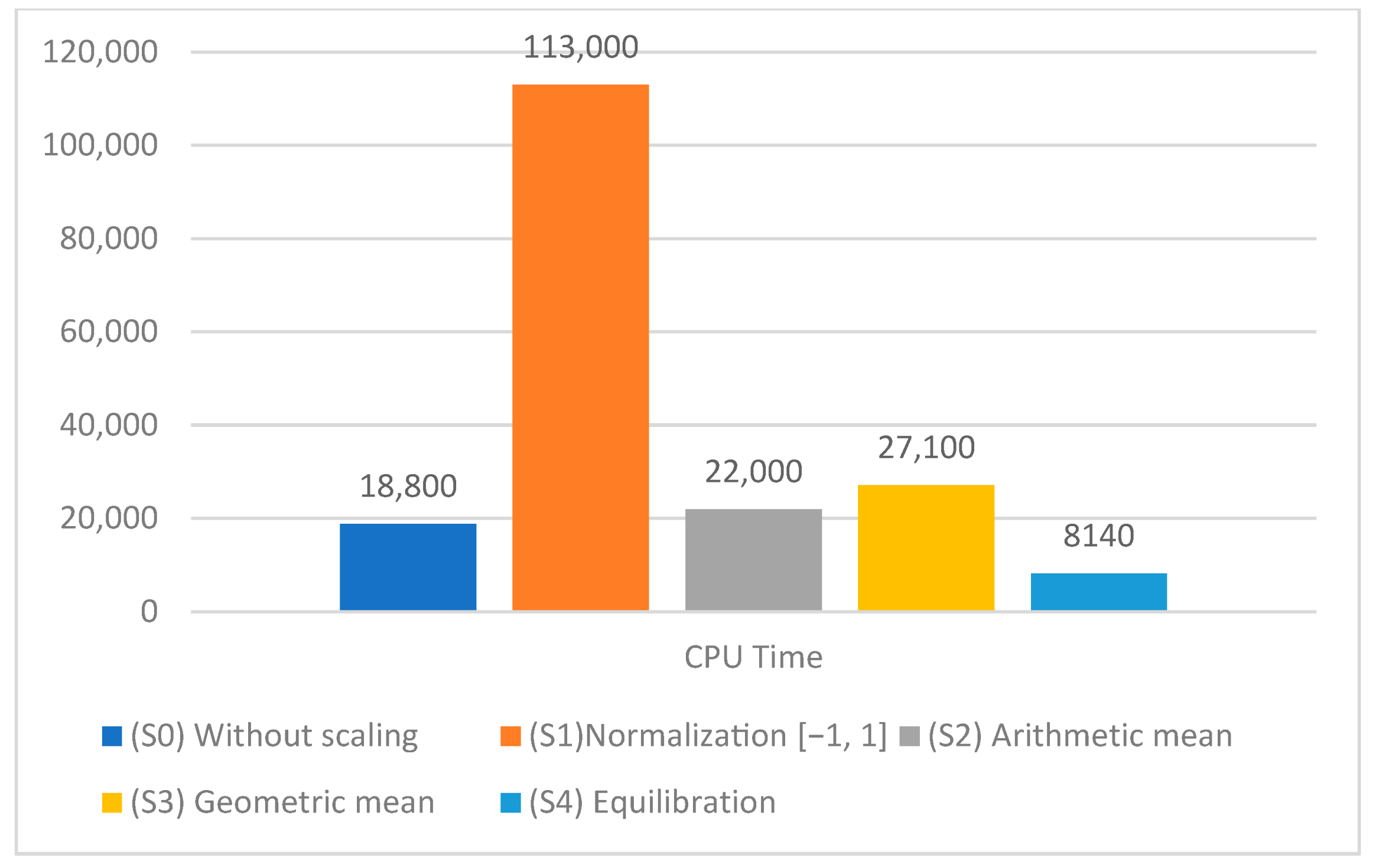
No	Symbol	Accuracy	CPU Time
1	(S0)	89.11	18,800
1	(S1)	98.24	113,000
2	(S2)	98.25	22,000
3	(S3)	98.24	27,100
4	(S4)	99.47	8140

and Figure 5 and Figure 6. In terms of accuracy and CPU time, the equilibration scaling technique clearly outperformed all other scaling techniques. In terms of precision, however, the equilibration scaling technique was the least accurate. According to CPU time, the normalization scaling in the range [−1, 1] was the greatest.

The accuracy rate of the proposed HHO-SVM model was compared to that of the conventional SVM employing a grid search technique in

Table 19. Accuracy comparison between HHO-SVM and Grid-SVM.

Symbol	Scaling Techniques	HHO-SVM Accuracy	Grid-SVM Accuracy
(S1)	Normalization [−1, 1]	98.24	96.49
(S2)	Arithmetic mean	98.25	98.42
(S3)	Geometric mean	98.24	98.59
(S4)	Equilibration	99.47	98.95

. For the scaling procedures S4, S2, S3, and S1, the accuracy rates of the proposed HHO-SVM model were 99.47, 98.25, 98.24, and 98.24, respectively. For the scaling approaches S4 and S1, the accuracy rates of the classic SVM with a grid search algorithm were 98.95 and 96.49, respectively.

The parallel version of the HHO-SVM algorithm was provided to reduce its running time. CPU timings for all scaling strategies produced by the HHO-SVM on different cores are shown in

Table 20. CPU time comparison between HHO-SVM and Grid-SVM.

Symbol	Scaling Techniques	HHO-SVM
		Core1	Core2	Core4
(S1)	Normalization [−1, 1]	91,600	47,461.14	23,073.04
(S2)	Arithmetic mean	8560	4703.30	2338.80
(S3)	Geometric mean	11,000	5820.11	2941.18
(S4)	Equilibration	3500	2023.12	980.39

and Figure 7.

In addition,

Table 21. Speedup on the WBCD database using the HHO-SVM with S1, S2, S3, and S4.

Symbol	HHO-SVM
	Core1	Core2	Core4
(S1)	1	1.93	3.97
(S2)	1	1.82	3.66
(S3)	1	1.89	3.74
(S4)	1	1.73	3.57

For the scaling techniques S4, S3, S2, and S1, the speedups for four cores were 3.57, 3.74, 3.66, and 3.97, respectively.

and Figure 8 show the speedup obtained by the HHO-SVM for all scaling strategies.

Table 22. A comparison between related works against to our model.

Study	Year	Method	Accuracy (%)
Tuba et al. [6]	(2016)	ABA-SVM	96.49 %
Aalaei et al. [7]	(2016)	GA-ANN	97.30%
S. Mandal [8]	(2017)	Logistic regression	97.90%
Liu et al. [10]	(2018)	ICS-SVM	98.83%
Agarap [11]	(2018)	GRU-SVM	93.80%
Dhahri et al. [15]	(2019)	GA-AB	98.23%
Telsang et al. [17]	(2020)	SVM	96.25%
Umme et al. [18]	(2020)	BATGSA-FNN	92.10%
Singh et al. [19]	(2020)	GWWOA-SVM	97.72%
Badr et al. [20]	(2021)	GWO-SVM	99.3%
Our study	(2023)	HHO-SVM	99.47%

shows that the performance of the presented HHO-SVM model against other related models developed in the literature, demonstrating the usefulness of our method. Table 22 shows that the classification accuracy of our created HHO-SVM diagnostic system is equivalent to or better than that of existing classifiers on the WBCD database.

8. Conclusions

Three achievements were proposed. The first achievement was a novel hybrid classifier (HHO-SVM), which was a combination of the Harris hawks optimization (HHO) and a support vector machine (SVM). In order to increase the HHO-SVM performance, the second goal was to compare three efficient scaling algorithms to the old normalizing methodology. The final contribution was to improve the efficiency of the HHO-SVM by adopting a parallel approach that employed the data distribution. On the Wisconsin Diagnosis Breast Cancer (WDBC) dataset, the proposed models were tested. The results showed that the HHO-SVM achieved a 98.24% accuracy rate with the normalization scaling technique, thus outperforming the results in [6,7,8,11,15,17,18,19]. On the other hand, the HHO-SVM achieved a 99.47% accuracy rate with the equilibration scaling technique, outperforming the results in [6,7,8,10,11,15,17,18,19,20]. Finally, on four CPU cores, the parallel HHO-SVM model delivered a speedup of 3.97. The proposed approach will be evaluated in various medical datasets in future research. In addition, we are attempting to incorporate various measuring techniques that will reduce the running time and improve the proposed diagnostic system’s efficiency.

References

- Sung, H.; Ferlay, J.; Siegel, R.L.; Laversanne, M.; Soerjomataram, I.; Jemal, A.; Bray, F. Global Cancer Statistics 2020: GLOBOCAN Estimates of Incidence and Mortality Worldwide for 36 Cancers in 185 Countries. CA Cancer J. Clin. 2021, 71, 209–249. [Google Scholar] [CrossRef] [PubMed]
- Marcano-Cedeño, A.; Quintanilla-Domínguez, J.; Andina, D. WBCD breast cancer database classification applying artificial metaplasticity neural network. Expert Syst. Appl. 2011, 38, 9573–9579. [Google Scholar] [CrossRef]
- Chen, H.-L.; Yang, B.; Liu, J.; Liu, D.-Y. A support vector machine classifier with rough set-based feature selection for breast cancer diagnosis. Expert Syst. Appl. 2011, 38, 9014–9022. [Google Scholar] [CrossRef]
- Chen, H.L.; Yang, B.; Wang, G.; Wang, S.J.; Liu, J.; Liu, D.Y. Support vector machine based diagnostic system for breast cancer using swarm intelligence. J. Med. Syst. 2012, 36, 2505–2519. [Google Scholar] [CrossRef] [PubMed]
- Bashir, S.; Qamar, U.; Khan, F.H. Heterogeneous classifiers fusion for dynamic breast cancer diagnosis using weighted vote based ensemble. Qual. Quant. 2015, 49, 2061–2076. [Google Scholar] [CrossRef]
- Tuba, E.; Tuba, M.; Simian, D. Adjusted bat algorithm for tuning of support vector machine parameters. In Proceedings of the 2016 IEEE Congress on Evolutionary Computation (CEC), Vancouver, BC, Canada, 24–29 July 2016; pp. 2225–2232. [Google Scholar] [CrossRef]
- Aalaei, S.; Shahraki, H.; Rowhanimanesh, A.; Eslami, S. Feature selection using genetic algorithm for breast cancer diagnosis: Experiment on three different datasets. Iran. J. Basic. Med. Sci. 2016, 19, 476–482. [Google Scholar]
- Mandal, S.K. Performance Analysis of Data Mining Algorithms for Breast Cancer Cell Detection Using Naïve Bayes, Logistic Regression and Decision Tree. Int. J. Eng. Comput. Sci. 2017, 6, 20388–20391. [Google Scholar]
- Muslim, M.A.; Rukmana, S.H.; Sugiharti, E.; Prasetiyo, B.; Alimah, S. Optimization of C4.5 algorithm-based particle swarm optimization for breast cancer diagnosis. J. Phys. Conf. Ser. 2018, 983, 012063. [Google Scholar] [CrossRef]
- Liu, N.; Shen, J.; Xu, M.; Gan, D.; Qi, E.-S.; Gao, B. Improved Cost-Sensitive Support Vector Machine Classifier for Breast Cancer Diagnosis. Math. Probl. Eng. 2018, 2018, 3875082. [Google Scholar] [CrossRef]
- Agarap, A.F.M. On breast cancer detection: An application of machine learning algorithms on the wisconsin diagnostic dataset. In Proceedings of the 2nd International Conference on Machine Learning and Soft Computing, Phuoc Island, Vietnam, 2–4 February 2018; pp. 5–9. [Google Scholar] [CrossRef]
- Huang, H.; Feng, X.; Zhou, S.; Jiang, J.; Chen, H.; Li, Y.; Li, C. A new fruit fly optimization algorithm enhanced support vector machine for diagnosis of breast cancer based on high-level features. BMC Bioinform. 2019, 20, 290. [Google Scholar] [CrossRef]
- Xie, T.; Yao, J.; Zhou, Z. DA-Based Parameter Optimization of Combined Kernel Support Vector Machine for Cancer Diagnosis. Processes 2019, 7, 263. [Google Scholar] [CrossRef]
- Rajaguru, H.; SR, C.S. Analysis of Decision Tree and K-Nearest Neighbor Algorithm in the Classification of Breast Cancer. Asian Pac. J. Cancer Prev. 2019, 20, 3777–3781. [Google Scholar] [CrossRef] [PubMed]
- Dhahri, H.; Al Maghayreh, E.; Mahmood, A.; Elkilani, W.; Nagi, M.F. Automated Breast Cancer Diagnosis Based on Machine Learning Algorithms. J. Health Eng. 2019, 2019, 4253641. [Google Scholar] [CrossRef] [PubMed]
- Hemeida, A.; Alkhalaf, S.; Mady, A.; Mahmoud, E.; Hussein, M.; Eldin, A.M.B. Implementation of nature-inspired optimization algorithms in some data mining tasks. Ain Shams Eng. J. 2020, 11, 309–318. [Google Scholar] [CrossRef]
- Telsang, V.A.; Hegde, K. Breast Cancer Prediction Analysis using Machine Learning Algorithms. In Proceedings of the 2020 International Conference on Communication, Computing and Industry 4.0 (C2I4), Bangalore, India, 17–18 December 2020; pp. 1–5. [Google Scholar] [CrossRef]
- Salma, M.U.; Doreswamy, N. Hybrid BATGSA: A metaheuristic model for classification of breast cancer data. Int. J. Adv. Intell. Paradig. 2020, 15, 207. [Google Scholar] [CrossRef]
- Singh, I.; Bansal, R.; Gupta, A.; Singh, A. A Hybrid Grey Wolf-Whale Optimization Algorithm for Optimizing SVM in Breast Cancer Diagnosis. In Proceedings of the 2020 Sixth International Conference on Parallel, Distributed and Grid Computing (PDGC), Waknaghat, India, 6–8 November 2020; pp. 286–290. [Google Scholar] [CrossRef]
- Badr, E.; Almotairi, S.; Salam, M.A.; Ahmed, H. New Sequential and Parallel Support Vector Machine with Grey Wolf Optimizer for Breast Cancer Diagnosis. Alex. Eng. J. 2021, 61, 2520–2534. [Google Scholar] [CrossRef]
- Badr, E.; Salam, M.A.; Almotairi, S.; Ahmed, H. From Linear Programming Approach to Metaheuristic Approach: Scaling Techniques. Complexity 2021, 2021, 9384318. [Google Scholar] [CrossRef]
- Badr, E.S.; Paparrizos, K.; Samaras, N.; Sifaleras, A. On the Basis Inverse of the Exterior Point Simplex Algorithm. In Proceedings of the 17th National Conference of Hellenic Operational Research Society (HELORS), Rio, Greece, 16–18 June 2005; pp. 677–687. [Google Scholar]
- Badr, E.S.; Paparrizos, K.; Thanasis, B.; Varkas, G. Some computational results on the efficiency of an exterior point algorithm. In Proceedings of the 18th National conference of Hellenic Operational Research Society (HELORS), Kozani, Greece, 15–17 June 2006; pp. 1103–1115. [Google Scholar]
- Badr, E.M.; Moussa, M.I. An upper bound of radio k-coloring problem and its integer linear programming model. Wirel. Netw. 2020, 26, 4955–4964. [Google Scholar] [CrossRef]
- Badr, E.; AlMotairi, S. On a Dual Direct Cosine Simplex Type Algorithm and Its Computational Behavior. Math. Probl. Eng. 2020, 2020, 7361092. [Google Scholar] [CrossRef]
- Badr, E.S.; Moussa, M.; Paparrizos, K.; Samaras, N.; Sifaleras, A. Some computational results on MPI parallel implementation of dense simplex method. Trans. Eng. Comput. Technol. 2006, 17, 228–231. [Google Scholar]
- Elble, J.M.; Sahinidis, N.V. Scaling linear optimization problems prior to application of the simplex method. Comput. Optim. Appl. 2012, 52, 345–371. [Google Scholar] [CrossRef]
- Ploskas, N.; Samaras, N. The impact of scaling on simplex type algorithms. In Proceedings of the 6th Balkan Conference in Informatics, Thessaloniki Greece, 19–21 September 2013; pp. 17–22. [Google Scholar] [CrossRef]
- Triantafyllidis, C.; Samaras, N. Three nearly scaling-invariant versions of an exterior point algorithm for linear programming. Optimization 2015, 64, 2163–2181. [Google Scholar] [CrossRef]
- Ploskas, N.; Samaras, N. A computational comparison of scaling techniques for linear optimization problems on a graphical processing unit. Int. J. Comput. Math. 2015, 92, 319–336. [Google Scholar] [CrossRef]
- Badr, E.M.; Elgendy, H. A hybrid water cycle-particle swarm optimization for solving the fuzzy underground water confined steady flow. Indones. J. Electr. Eng. Comput. Sci. 2020, 19, 492–504. [Google Scholar] [CrossRef]
- Tapkan, P.; Özbakır, L.; Baykasoglu, A. Bee algorithms for parallel two-sided assembly line balancing problem with walking times. Appl. Soft Comput. 2016, 39, 275–291. [Google Scholar] [CrossRef]
- Tian, T.; Gong, D. Test data generation for path coverage of message-passing parallel programs based on co-evolutionary genetic algorithms. Autom. Softw. Eng. 2016, 23, 469–500. [Google Scholar] [CrossRef]
- Maleki, S.; Musuvathi, M.; Mytkowicz, T. Efficient parallelization using rank convergence in dynamic programming algorithms. Commun. ACM 2016, 59, 85–92. [Google Scholar] [CrossRef]
- Sandes, E.F.D.O.; Boukerche, A.; De Melo, A.C.M.A. Parallel Optimal Pairwise Biological Sequence Comparison. ACM Comput. Surv. 2016, 48, 1–36. [Google Scholar] [CrossRef]
- Truchet, C.; Arbelaez, A.; Richoux, F.; Codognet, P. Estimating parallel runtimes for randomized algorithms in constraint solving. J. Heuristics 2016, 22, 613–648. [Google Scholar] [CrossRef]
- Połap, D.; Kęsik, K.; Woźniak, M.; Damaševičius, R. Parallel Technique for the Metaheuristic Algorithms Using Devoted Local Search and Manipulating the Solutions Space. Appl. Sci. 2018, 8, 293. [Google Scholar] [CrossRef]
- Jiao, S.; Gao, Y.; Feng, J.; Lei, T.; Yuan, X. Does deep learning always outperform simple linear regression in optical imag-ing? Opt. Express 2020, 28, 3717–3731. [Google Scholar] [CrossRef] [PubMed]
- Chauhan, D.; Anyanwu, E.; Goes, J.; Besser, S.A.; Anand, S.; Madduri, R.; Getty, N.; Kelle, S.; Kawaji, K.; Mor-Avi, V.; et al. Comparison of machine learning and deep learning for view identification from cardiac magnetic resonance images. Clin. Imaging 2022, 82, 121–126. [Google Scholar] [CrossRef]
- Sain, S.R.; Vapnik, V.N. The Nature of Statistical Learning Theory; Springer Science & Business Media: Berlin/Heidelberg, Germany, 1996; Volume 38. [Google Scholar]
- Cristianini, N.; Shawe-Taylor, J. An Introduction to Support Vector Machines and Other Kernel-Based Learning Meth-Ods; Cambridge University Press: Cambridge, UK, 2000. [Google Scholar]
- Boser, B.E.; Guyon, I.M.; Vapnik, V.N. A training algorithm for optimal margin classifiers. In Proceedings of the Fifth Annual Workshop on Computational Learning Theory, Pittsburgh, PA, USA, 27–29 July 1992; pp. 144–152. [Google Scholar] [CrossRef]
- Heidari, A.A.; Mirjalili, S.; Faris, H.; Aljarah, I.; Mafarja, M.; Chen, H. Harris hawks optimization: Algorithm and applications. Futur. Gener. Comput. Syst. 2019, 97, 849–872. [Google Scholar] [CrossRef]
- UCI Machine Learning Repository. Breast Cancer Wisconsin (Diagnostic) Data Set 1995. Available online: https://archive.ics.uci.edu/dataset/17/breast+cancer+wisconsin+diagnostic (accessed on 1 January 2015).
- Chang, C.; Lin, C. LIBSVM: A Library for Support Vector Machines. ACM Trans. Intell. Syst. Technol. 2013, 2, 1–27. [Google Scholar] [CrossRef]
- Salzberg, S.L. On Comparing Classifiers: Pitfalls to Avoid and a Recommended Approach. Data Min. Knowl. Discov. 1997, 1, 317–328. [Google Scholar] [CrossRef]