Article

Transient Dynamics in Counter-Rotating Stratified Taylor–Couette Flow

by
Larry E. Godwin
1,
Philip M. J. Trevelyan
1,
Takeshi Akinaga
2 and
Sotos C. Generalis
1,*
1
Department of Applied Mathematics and Data Science, School of Engineering and Applied Science, Aston University, Birmingham B4 7ET, UK
2
Faculty of Engineering Science, Akita University, 1-1 Tegatagakuen-machi, Akita 010-8502, Japan
*
Author to whom correspondence should be addressed.
Mathematics 2023, 11(14), 3250; https://doi.org/10.3390/math11143250
Submission received: 19 June 2023 / Revised: 19 July 2023 / Accepted: 22 July 2023 / Published: 24 July 2023
(This article belongs to the Section Probability and Statistics)

Abstract

:
This study focuses on the investigation of stratified Taylor–Couette flow (STCF) using non-modal analysis, which has received relatively limited attention compared to other shear flows. The dynamics of perturbations under different temperature conditions are explored, and their patterns of amplification are analyzed. The study highlights the correlation between flow configurations, emphasizing the similarity in transient dynamics despite different speed ratios. The subcritical effects of thermal stratification on disturbance dynamics are examined, considering the interplay between viscous and buoyancy effects counteracted by strong centrifugal forces. It is found that increasing the wall temperature beyond a critical value leads to buoyancy forces dominating, resulting in a linear increase in the amplification factor. The research reveals significant deviations from previous results, indicating the significant role of temperature stratification.

1. Introduction

The transition from laminar to turbulent fluid flow has been of interest for over a century. Beyond the laminar state, fluid flows can exhibit several states before they reach a turbulent state. These states have played a role in making significant contributions in industries such as automobile, civil, aerospace, and others. To address the instabilities arising from flow disturbances, a multitude of mathematical techniques have been developed within hydrodynamic stability theory [1,2].
Numerical and analytical methods, including bifurcation theory and other suitable approaches, have been employed to identify these flow patterns [3,4]. Among the various techniques used, the transient growth method has gained extensive utilization in the exploration of subcritical transitions in fluid flow, proving to be highly successful over several decades. This method has been invaluable in capturing and elucidating phenomena associated with stability problems in fluid flows that cannot be effectively addressed by linear stability theory alone [5,6,7,8,9].
The plane Couette and pipe Poiseuille flows are known to be stable for all Reynolds numbers within the theoretical mathematical framework of linear stability analysis, but in practice, these flows become turbulent for sufficiently large Reynolds numbers, as accounted for by Romanov [10], Davey [11], Drazin and Reid [12] and recent studies by others [13,14]. In practice, the plane Poiseuille flow does exhibit an instability at a critical Reynolds number Re c 2300, but theoretically this phenomenon is observed at a much larger value, Re c 5772, at which the so-called Tollmien–Schlichting wave depicting an unstable mode appears [15,16]. The inconsistency in results has been attributed to the non-normality of the linearized Navier–Stokes operator. It is known that the non-normality is responsible for the spike (i.e., transient growth) in the growth rate within the linear regime that eventually triggers the transition from laminar to turbulent flow. This behavior is widely known as a subcritical transition or bypass transition [5,17,18]. The non-normal route to turbulence has raised many concerns in the literature from different schools of thought [7,19,20], conversely, Reddy and Henningson [21] objectively addressed the issues with insightful results for two- and three-dimensional plane Couette and Poiseuille flows. The utilization of the transient growth method for investigating subcritical bifurcations has witnessed widespread adoption and significant advancements over the last two decades, with both theoretical and experimental justifications [8,22,23,24].
The circular Couette flow, often known as Taylor–Couette flow (TCF), has been widely studied experimentally and theoretically [25,26,27,28,29]. The TCF problem has been known to be one of the pioneering problems of hydrodynamic stability for several decades, since the early experimental and theoretical works of Taylor [30]. In 1965, Coles [31] experimentally investigated the transition of viscous flow in concentric cylinders and reported that at certain Reynolds numbers, where the linear theory predicted laminar flow, there exists spiral turbulence in the counter-rotating flow [31]. In the following year, Van Atta [32] carried out similar experiments on the spiral transition of the flow and obtain related results. These results were confirmed experimentally later, in 1989, by Hegseth et al. [33] and later, in 2002, by Prigent et al. [34].
The non-normality problem of the TCF linear operator was initially investigated by Grebhardt and Grossmann in 1992 [26]. However, Hristova et al. [35] conducted a comprehensive investigation of this phenomenon using pseudospectral analysis. In 2002, Meseguer [36] examined the transient energy growth associated with the parametric regime reported by Coles [31] and observed a significant amplification of the transient energy in the counter-rotating regime, which aligned well with Coles’s [31] experimental findings. It was discovered that the non-axisymmetric modes experience greater amplification and they could potentially trigger the subcritical transition to turbulence [19,36]. Maretzke et al. [37] further expanded on this perspective through numerical and analytical methods. The authors explored the transient energy growth rates of the modes across all TCF regimes and established a universal Re 2 / 3 scaling. Additionally, it was established that the linear stability and transient growth rate remained unaffected by the ratio of the cylinders’ rotation rates in the limit where there was no axial perturbation dependency.
However, there has been a significant lack of attention given to the application of non-modal analysis in the context of stratified Taylor–Couette flow (STCF). Thus, the primary objective of this research is to extend the existing experimental work conducted by Cole [31] in the domain of thermal convection by employing non-modal analysis techniques. Building upon the configuration reported by Meseguer [36], we introduce radial heating and proceed with a comprehensive investigation of the subcritical phenomena associated with counter-rotating flows. This article specifically focuses on the optimal transient growth rate observed in counter-rotating stratified Taylor–Couette flow, with a particular emphasis on non-axisymmetric perturbations. To provide a comprehensive understanding of the topic, Section 2 presents a concise overview of the governing equations underlying the Taylor–Couette problem. The derived model is then linearized in Section 3. Section 4 offers an in-depth discussion of the results obtained from our investigation. Finally, the overall conclusions drawn from this study are summarized in Section 5.

2. Mathematical Formulation

2.1. Model

We examine the behavior of an incompressible fluid with kinematic viscosity μ , and a density ρ = ρ o + ρ , which is contained between two concentric cylinders of infinite height, where ρ o is the average density of the fluid and ρ is the variation in the density. The inner cylinder has a radius r i , and rotates at an angular velocity Ω i > 0 , while the outer cylinder has a radius r o , and rotates at an angular velocity Ω o < 0 . Additionally, we assume a negative temperature gradient with an inner temperature T i = T ¯ + Δ T / 2 , and an outer temperature T o = T ¯ Δ T / 2 , as depicted in Figure 1, where T ¯ is the ambient temperature and Δ T is the temperature difference between the two cylinders. Thus, the model is governed by the incompressible Navier–Stokes equations for rapidly rotating flows, as described by Lopez et al. [28,38,39]:
ρ o ( t v + ( v · ) v ) = Π + μ 2 v + ρ Π + ρ ( v · ) v ,
· v = 0 , and
t T + ( v · ) T = κ 2 T ,
where κ is the thermal diffusivity of the fluid; Π = p + ρ o Φ is composed of the gradient terms pressure p, and constant gravitational potential ρ o Φ .
The boundary conditions are given as:
v · e θ = Ω i on r = r i and v · e θ = Ω o on r = r o .
Equation (1) is defined in the stationary reference frame and the last term, ( ρ ( v · ) v ), describes the centrifugal buoyancy contribution of the flow. This term is necessary in order to accurately account for strong vortex dynamics or flows with rapidly rotating walls.

2.2. Boussinesq Approximation

The system is defined by a cylindrical coordinate system ( r , θ , z ) . We proceed with the Boussinesq assumption by ignoring density variations in the flow, and we only keep density contributions from the gravitational and centrifugal terms. Furthermore, we assume a constant gravitational acceleration, g, in the vertical direction, z. By assuming that the temperature has a linearly decreasing effect on the density, we have:
ρ = ρ o ( 1 β T )
where β = ( 1 / ρ o ) ρ / T | ρ = ρ o is the coefficient of thermal expansion. Since ρ = ρ o + ρ , we have:
ρ = ρ o β T .
Now, applying (6) to the buoyancy term in (1) and using Φ = g z , we have:
t v + ( v · ) v = Π + ν 2 v β g T e z β T ( v · ) v .

2.3. Nondimensionalization

In this section, we proceed by converting Equations (2), (3), and (7) to dimensionless forms by using Δ T , the gap-width d = r o r i , d 2 / ν , and ( ν / d ) 2 as the temperature, length, viscous time, and reduced pressure p / ρ o scaling factors, respectively. The inner r i and outer r o radii are expressed in dimensionless form as η / ( 1 η ) and 1 / ( 1 η ) , respectively. With these scaling factors we obtained the new dimensionless parameters listed in Table 1. In addition, we introduce a dummy variable Υ { 0 , 1 } into the equation:
t v + ( v · ) v = p + 2 v + Υ Gr T e z + Υ ϵ T ( v · ) v ,
· v = 0 ,
t T + ( v · ) T = 1 Pr 2 T ,
where e z is the unit vector in the axial direction z.
If Υ is 1, then (8) describes the STCF system and if it is 0, then it defines the TCF system without stratification. Thus, we use these parameters and the dimensionless Equations (8)–(10) in subsequent sections for our analysis and discussion.

2.4. Basic Equations

Given the nondimensional equations, let the velocity be expressed as v = u e r + v e θ + w e z in cylindrical coordinates, where u, v, and w are the radial, azimuthal, and axial components of the velocity, respectively, and e r and e θ are the unit vectors in the r, θ , and z directions. The basic velocity U , becomes:
U = U b e r + V b e θ + W b e z
and the basic components of the velocity U b , V b , and W b correspond to the respective radial, azimuthal, and axial basic profiles. Thus, we proceed by deriving expressions for the basic profiles by assuming that U is independent of time t, and the azimuthal θ and axial z directions. In addition, in order to have a constant pressure gradient in the axial direction, we impose the zero mass flux constraint,
r i r o r W b ( r ) d r = 0
and thus, with these assumptions we obtain the following analytical solutions:
U b ( r )   =    0
V b ( r )   =    A r + B r
W b ( r )   =    Gr Υ ( 1 η ) 2 [ C ( ( r ( 1 η ) ) 2 η 2 )                    + C ( 1 η 2 ) + 1 8 ( 1 ( r ( 1 η ) ) 2 ) 2 T b ( r ) 1 ]
T b ( r )   =    ln ( ( r / η ) ( 1 η ) ) ln ( η ) + 1 2
where V b , W b , and T b remain the same solutions introduced in the related literature. The constants A, B and C are given by the expressions:
A = Re o η Re i 1 + η , B = η ( Re i η Re o ) ( 1 η ) ( 1 η 2 ) ,
and
C = ( η 2 3 ) ( η 2 1 ) + 4 ln ( η ) 16 ( η 2 1 ) ( ( 1 + η 2 ) ln ( η ) + 1 η 2 ) .

3. Linearization

Furthermore, we suppose that the basic state is subjected to an infinitesimal perturbation:
v = U + δ v ˜ ,
p = P b + δ p ˜ ,
T = T b + δ T ˜ ,
where δ is assumed to be a very small constant and v ˜ , p ˜ and T ˜ are the residues (fluctuations) of the velocity, pressure and temperature, respectively. We substitute Equations (19)–(21), into the dimensionless governing Equations (8)–(10). We then proceed by collecting the O( δ ) terms and ignore higher-order terms. Thus, the linearized equations become:
t v ˜ = p ˜ + 2 v ˜ + Υ G T ˜ e z + ( Υ ϵ T ˜ 1 ) ( ( U · ) v ˜ + ( v ˜ · ) U ) ,
· v ˜ = 0 ,
t T ˜ = 1 Pr 2 T ˜ ( U · ) T ˜ ( v ˜ · ) T b .
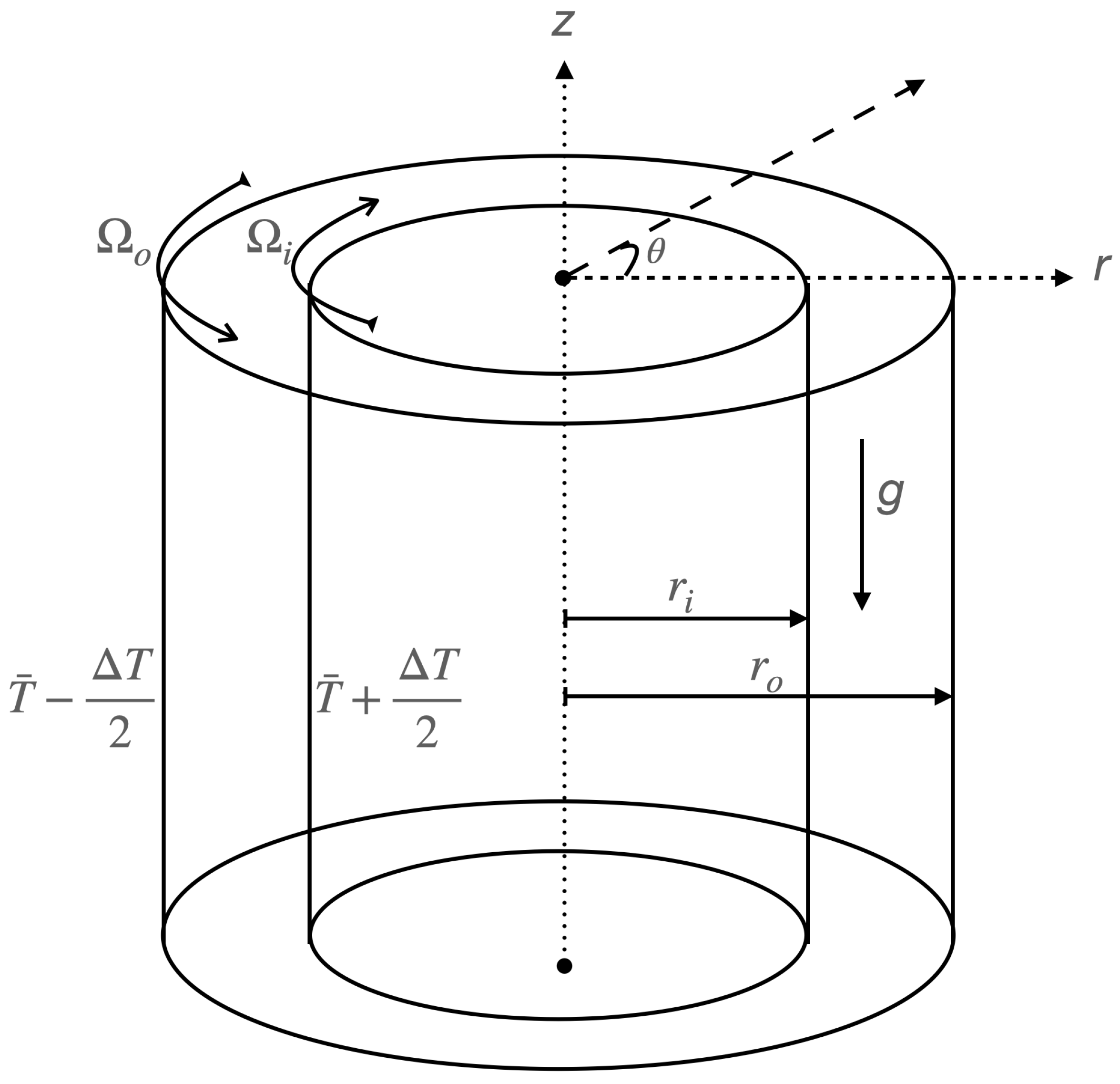
Our objective is to describe the transition of Taylor–Couette flow from laminar to turbulent flow. In particular, we seek to identify any differences between isothermal and stratified Taylor–Couette flow. To facilitate our analysis, and expecting harmonic motion, we utilize the Fourier transform in the azimuthal θ and axial z directions, while we employ the Gauss–Lobatto collocation point Chebyschev polynomial expansion in the radial direction r; see Figure 1. Based on these considerations, we propose the following functional forms:
v ˜ v ^ ( r , t ) e i ( n θ + k z ) , p ˜ p ^ ( r , t ) e i ( n θ + k z ) , T ˜ T ^ ( r , t ) e i ( n θ + k z )
where the pressure p ˜ , temperature T ˜ , and velocities u ˜ , v ˜ , and w ˜ are functions of the radial, azimuthal, and axial coordinate directions. Furthermore, n N and k R are the azimuthal and axial wavenumbers, respectively. The frequencies of the disturbance are characterized by the wavenumbers. The wavelengths in the homogeneous directions θ and z are L θ = 2 π / n and L z = 2 π / k , respectively. Thus, we proceed by substituting the above functional forms into the linearized Equations (22)–(24), which after further simplification become:
u ^ t = p ^ r + F ( n , k , Υ ) u ^ 2 i n r 2 2 V b r ( 1 Υ ϵ T b ) v ^ Υ ϵ V b 2 r T ^ ,
v ^ t = i n p ^ r + F ( n , k , Υ ) v ^ + 2 i n r 2 ( 1 Υ ϵ T b ) V b r + V b r u ^ ,
w ^ t = i k p ^ + F ( n , k , Υ ) + 1 r 2 w ^ W b r ( 1 Υ ϵ T b ) u ^ + Υ Gr T ^ ,
D + u ^ + i n r v ^ + i k w ^ = 0 ,
T ^ t = 1 Pr D + D n 2 r 2 k 2 i Pr n V b r + k W b T ^ T b r u ^ ,
where
F ( n , k , Υ ) = D + D n 2 + 1 r 2 k 2 i n V b r + k W b ( 1 ϵ Υ T b ) ,
D = d / d r , and D + = D + 1 / r . Manipulating Equations (25)–(29), we can represent the solenoidal system of equations in a compact form as an initial value problem:
t B q ^ = A q ^ ,
where A and B are defined in Appendix B. By assuming a solution of the form
v ^ = v ˘ ( r ) e λ t , p ^ = p ˘ ( r ) e λ t , and T ^ = T ˘ ( r ) e λ t .
We transform the initial value problem to a generalized eigenvalue problem:
λ q ^ = L q ^ and L = B 1 A .
The eigenvalues are complex and define the temporal linear stability of the flow. That is, if the real parts of all eigenvalues are negative, the flow is linearly stable and the amplitude of the perturbations will decay in time. Furthermore, if there exists an eigenvalue λ whose real part is positive, then the flow is unstable and the amplitude of the perturbation will grow in time. We assume that the perturbation of the velocity and temperature of the fluid motion must vanish at the walls:
v ˘ ( r i ) = v ˘ ( r o ) = T ˘ ( r i ) = T ˘ ( r o ) = 0 .

4. Numerical Results

The amplification factor, often denoted as G 0 , is a fundamental concept in the study of transient growth in fluid dynamics. It quantifies the maximum amplification of perturbations or disturbances in a given flow system over a certain time interval. Transient growth refers to the temporary amplification of perturbations in a flow before they eventually decay or become insignificant. This phenomenon is particularly relevant in the subcritical transition to turbulence, where small disturbances can trigger the onset of turbulent behavior. The amplification factor, G 0 , represents the maximum energy amplification that can be achieved by the optimal initial perturbations within a specified time frame. It characterizes the efficiency of energy transfer from the mean flow to the perturbations. A larger value of G 0 indicates a higher potential for transient growth and the presence of stronger amplification mechanisms in the flow. The computation of G 0 , as defined in Appendix A, involves solving an eigenvalue problem or performing a non-modal analysis, depending on the nature of the flow and the mathematical framework employed. By determining the optimal initial conditions and analyzing the linearized equations governing the flow, G 0 can be evaluated. In addition, the structures and modes that contribute most significantly to the amplification can be identified. In our study, we employed well-established approaches from the literature to compute the amplification factor G 0 . These approaches have been widely used and validated in previous research, providing reliable and effective methods for evaluating the maximum amplification of disturbances in fluid flows. By utilizing these established techniques, we ensure the accuracy and robustness of our calculations, allowing us to gain valuable insights into the transient growth and stability characteristics of the flow system under investigation [5,40,41].
The configuration is chosen so that our results can compare well with earlier studies of Taylor–Couette flow (TCF) without stratification [35,36,37]. Hereafter, we apply stratification to the problem to investigate the behavior of the transient energy growth of the flow. Thus, we continue with an equivalent configuration used by Meseguer [36] for the study of energy transient growth in the TCF problem. We choose fixed values of η = 0.881 , ϵ = 0.067 , and Pr = 68 , and various values of Gr along with various wavenumber pairs ( n [ 0 , 15 ] , k [ 0 , 15 ] ). In addition, we consider specific counter-rotating pairs of values for Re i and Re o from the set of the most significant pairs reported by Meseguer [36] for the TCF case. Furthermore, for proper justification of this investigation, we consider the symmetry introduced due to the periodic assumption made for the azimuthal (i.e., the SO(2)-symmetry because of the invariance of the system with respect to the azimuthal rotation about the z-axis) and axial (i.e., the O(2)-symmetry because of the invariance of the system with respect to the reflections and translations of the axial axis) coordinate directions.
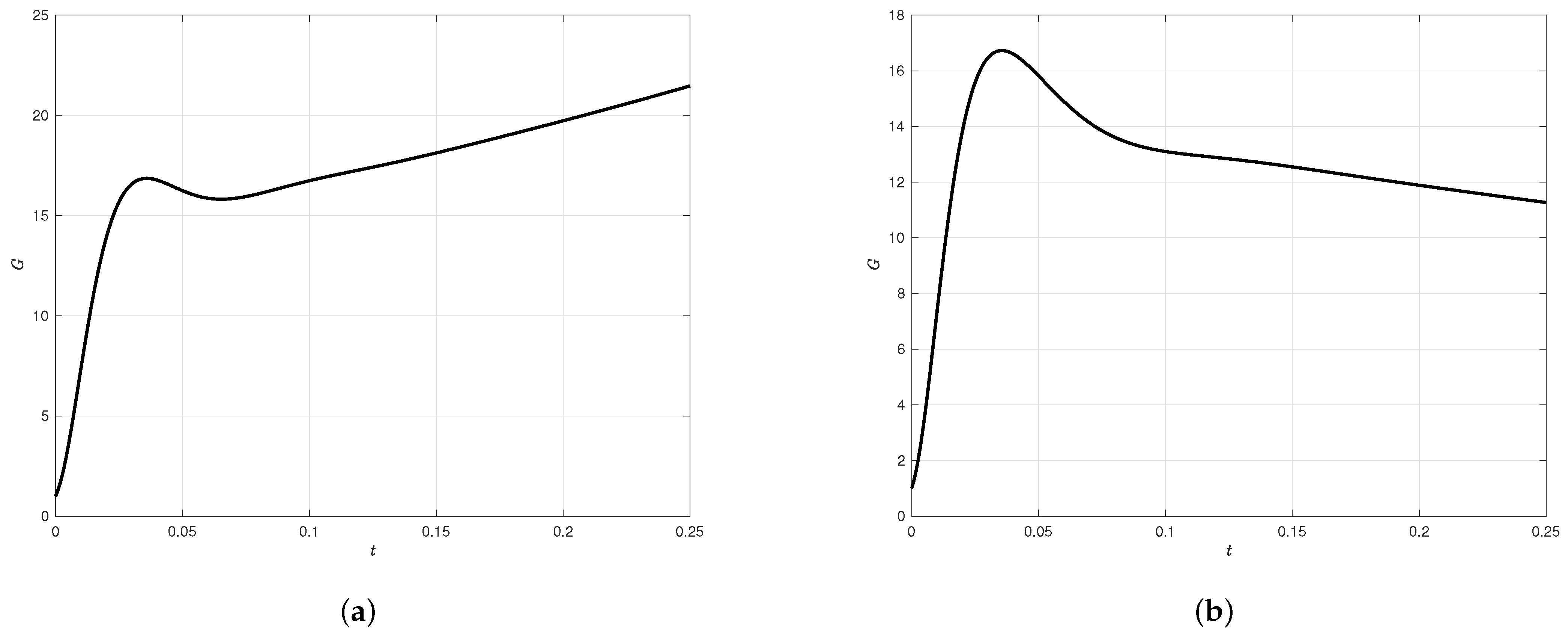
Due to the fact that no experimental work exists for the choice of configuration to which we can compare our results, we have introduced a parameter Υ in the governing dimensionless equation with values chosen to be either 0 or 1. The value of Υ is set to 0 in order to compare our findings with already existing results obtained for TCF [35,37]. The results, as indicated in Figure 2, are in perfect agreement with the results reported by Hristova et al. [35], Meseguer [36], and recently by works of Maretzke et al. [37]. In addition, we verify that the eigenvalues of the STCF case are in perfect agreement with Lopez [38], and McFadden et al. [38].
The nondimensional scheme we used is similar to Meseguer [36] and Maretzke et al. [37], but is slightly different from the scales used by Hristova et al. [35]. Thus, we made the conversions Re i alt = 2 Re i and Re o alt = 2 Re o / η in computing the results with those reported by Hristova et al. [35] as performed by others [36,37]. This is because Hristova et al. [35] used a scale of d / 2 to nondimensionalize the length and fix the angular rotation speed in defining the problem.
Meseguer [36] and Maretzke et al. [37] reported that close to the region where Re i = η Re o (i.e., the cylinders rotate at the same speed) no transient growth is observed. However, it is observed that the situation is different when the temperature increases beyond a certain threshold. There exists an amplification of the perturbations at specific times for different relative counter-rotating speeds in the presence of temperature variations. We continue by applying radial heating to the TCF problem and investigate the effect of the thermal stratification for various Grashof, Gr, numbers with specific counter-rotating pairs Re i , Re o and wavenumbers. 
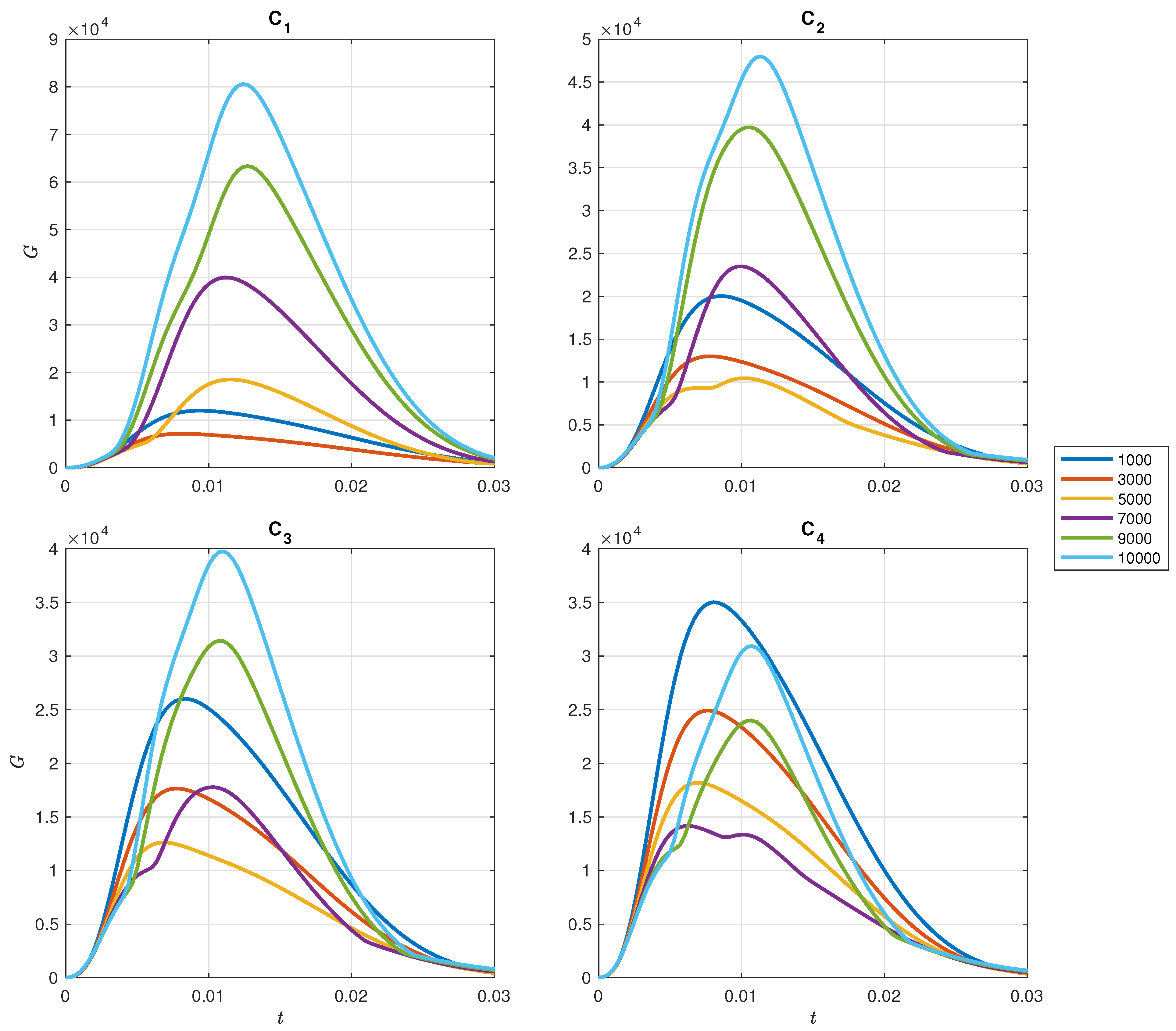
Figure 3 shows the amplification factor G against t for the four different configurations C 1 to C 4 for various values of Gr.
We find that G has a minimum around Gr = 3250 for configuration C 1 , around Gr = 4800 for configuration C 2 , around Gr = 5750 for configuration C 3 , and around Gr = 7150 for configuration C 4 . These results are verified explicitly in Figure 4b. 
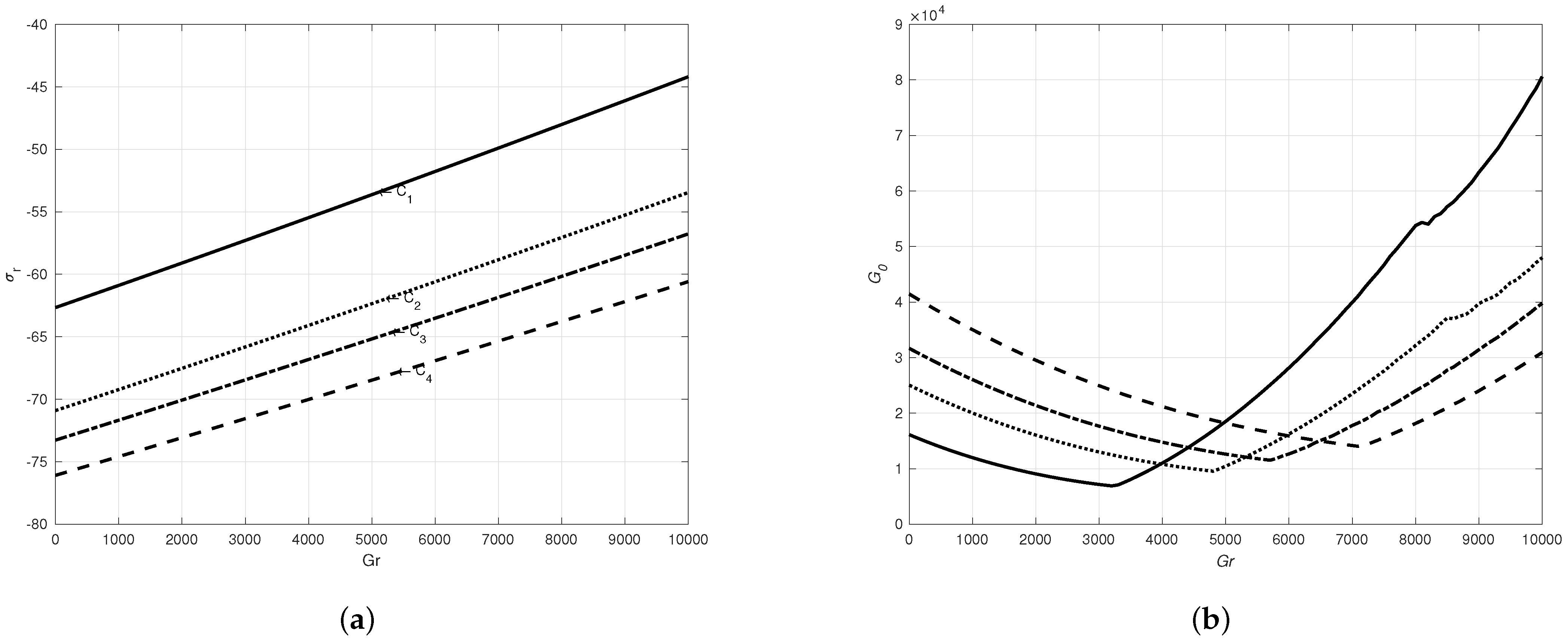
Figure 4 shows that as the temperature increases, the amplification of the perturbations monotonically decay, before reaching a turning point where it enters a new phase and begins increasing monotonically with temperature.
The growth rate shows a linear relationship with Gr in all configurations, as evident from Figure 4a. The growth rate remains consistently negative across all values of Gr, indicating that the fluid flow is linearly stable within the considered range of flows and implying that buoyancy does not induce a linear instability. Figure 4a clearly demonstrates an increase in the growth rate as Gr increases, which aligns with the proportional relationship between G 0 and Gr, as illustrated. We observe in Figure 4b that initially there is an observable downward trend in the linear decay of G 0 as Gr increases until it reaches a critical value Gr. Beyond this critical value, a linear increase in G 0 is observed as Gr continues to rise. By examining the decay phase boundaries, the order of G 0 for each configuration can be represented by the expression G 0 ( C 4 ) > G 0 ( C 3 ) > G 0 ( C 2 ) > G 0 ( C 1 ) . Similarly, for the increasing phase, the order of G 0 can be characterized as G 0 ( C 4 ) < G 0 ( C 3 ) < G 0 ( C 2 ) < G 0 ( C 1 ) .
An intriguing observation depicted in Figure 4b is the relationship between C 1 and the other configurations, namely, C 2 , C 3 , and C 4 , with respect to their ratio and the magnitude of their growth rates. Notably, there is a bigger difference in the order of growth rates between C 1 and C 2 when compared to the difference between C 2 and C 3 across all Gr values. The consistency in the proportionality of their speed ratio suggests that their growth rates should exhibit similar differences, in the same order of magnitude. This observation could be due to the influence of buoyancy-induced contributions captured in the amplification reflected by G 0 .
The underlying behavior of the fluid motion can be attributed to an internal subcritical phenomenon because of the induced thermal stratification on the dynamics of the disturbances. During the decay phases of the amplification factor, it is evident that the combination of viscous and buoyancy influences the amplitude of the perturbations.
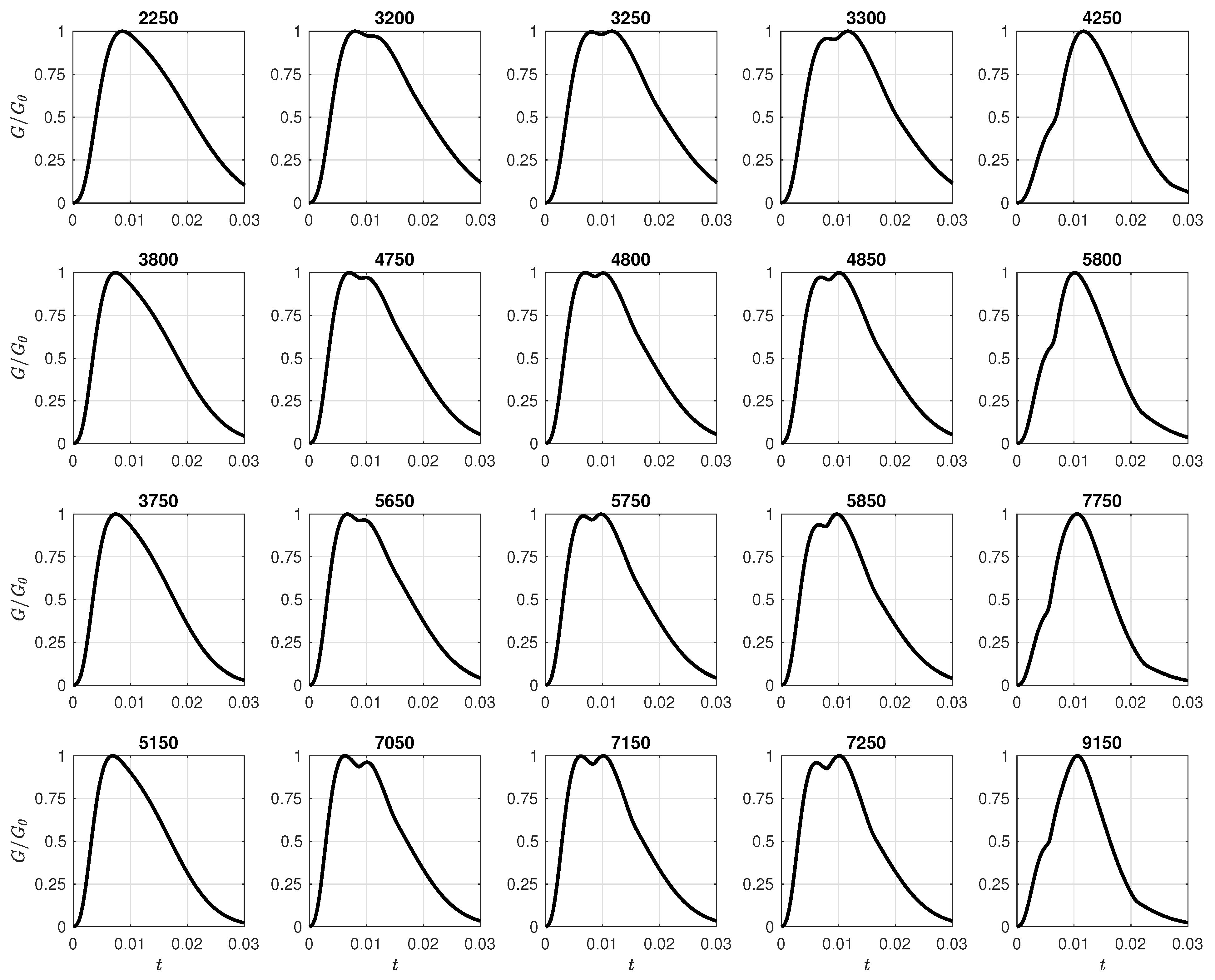
In Figure 5, the amplification factor G is depicted to illustrate its growth as Gr increases. Each row in the sequence of plots represents the evolving behavior of G as Gr increases. The first column has the values Gr = 2250, 3800, 3750, and 5150 and the last column has the values Gr = 4250, 5800, 7750, and 9150. They have Gr values slightly distant from the turning points, Gr = 3250, 4800, 5750, 7150 showcasing a single peak. Additionally, the plots in the second and fourth columns demonstrate two distinct behaviors in their evolution. Notably, the second column of plots display the emergence of a new crest on the wave front. This new crest continues to grow until it surpasses the initial crest in amplitude, eventually becoming the sole peak after the turning point for sufficiently high Gr values. The third column has used a value of Gr where both crescents exhibit similar amplitudes. The initial crest gradually merges into the latter one, and with further increases in Gr, the former completely disappears due to induced buoyancy disturbances.
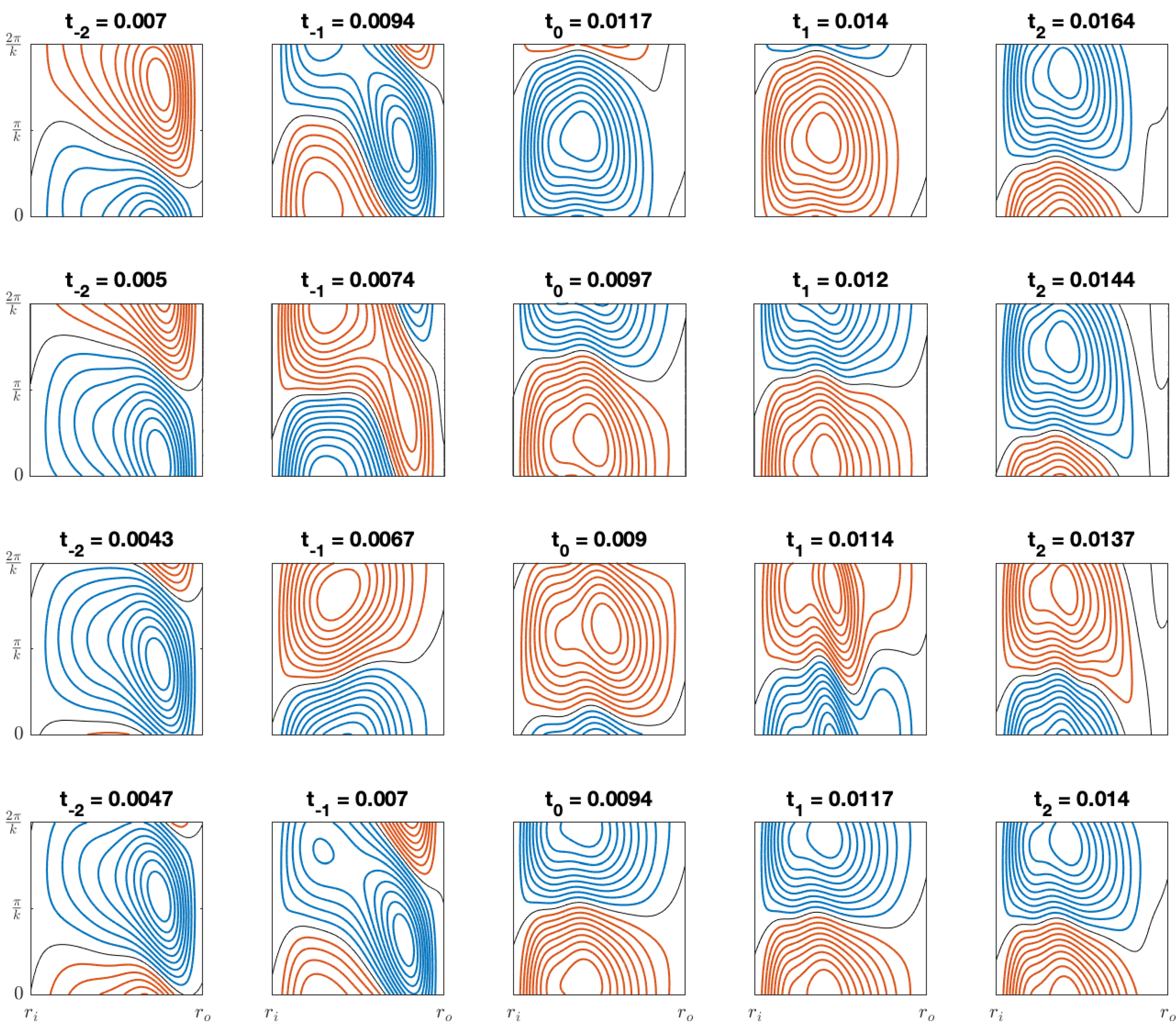
In Figure 6, we illustrate contour plots of the amplified perturbations in the radial velocity u ˘ at the value of Gr when G = G 0 .
The sequence of contour plots follows that of Figure 5 for C 1 to C 4 . Notice t 2 , t 1 , t 0 , t 1 , and t 2 follow an arithmetic progression, where t 0 is defined as the time when G = G 0 . We see in Figure 6, that at G = G 0 we have a reversal in the rotational direction of the perturbed flow.

5. Conclusions

Over the past twenty years, researchers have widely utilized non-normal analysis to investigate the linear transient characteristics of wall-bounded flows, particularly shear flows. However, there has been a relatively limited focus on applying this approach to examine the behavior of stratified Taylor–Couette flow (STCF).
This study aims to explore the dynamics of perturbations under different temperature conditions and analyze their patterns of amplification. Here we emphasize the correlation between various flow configurations, highlighting their similarity in transient dynamics despite differing speed ratios. Additionally, we investigate the subcritical effects of thermal stratification on the dynamics of the disturbances. The interplay between viscous and buoyancy effects, counteracted by strong centrifugal forces, is found to influence the growth and decay of the amplification factor. As the temperature increases beyond a turning point, buoyancy forces become dominant, leading to a linear increase in the amplification factor. The findings of this study reveal that incorporating temperature into the analysis significantly alters the expected outcomes, deviating considerably from the results obtained by Meseguer [36] and Coles [31]. This supports the notion that buoyancy, induced by the stratification of temperature variation, plays an important role. The transient analysis suggests the presence of complex dynamical phenomena specific to transient dynamics, which cannot be captured by solely focusing on the growth rates of the eigenvalues. An important result of our work is that we have identified the possibility of a two-dimensional subcritical bifurcation in STCF.
Transient growth of linearly stable disturbances is believed to play an important role in the subcritical transition of laminar boundary layers and the self-sustained nature of boundary layer fluctuations in a fully turbulent flow that the modal analysis might not capture within its operational framework. Indeed, our work shows that this is possible for the case of Taylor–Couette flow that has the additional influence of stratification.
In fact, we have performed direct numerical simulations (DNS) and have established that two-dimensional subcritical states are possible for the ubiquitous flow considered in this manuscript. Differences between the linearized theory of the present work and DNS are attributed to nonlinear advection mechanisms. A further investigation of this phenomenon is ongoing.
The transient growth phenomenon refers to an algebraic amplification of small-amplitude disturbances prior to an exponential decay farther downstream, that the full linearized modal mechanism does not capture. Therefore, transient growth has been proposed as a likely mechanism behind laminar–turbulent transition scenarios that cannot be elucidated by the classical paradigm of hydrodynamic instabilities. In fact, our work tackles the case where competition between hydrodynamic and convective instabilities is also present.
We show that the competition between convective and purely hydrodynamic instabilities through transient growth might play an important role in the self-generation of turbulence in fully turbulent wall shear flows through the subcritical generation of nonlinear states as predicted by the fully nonlinear Navier–Stokes equations [39]. This does not mean that transient growth is an alternative to the sequential approach to the turbulent regime, but rather an aid to generating additional branches to such a deterministic approach to turbulence that the sequence of bifurcation approach (SBA) offers. There is of course the alternative approaches by [42] that attempt to explain fully developed turbulence.

Author Contributions

Conceptualization, L.E.G.; methodology, L.E.G.; software, L.E.G.; validation, L.E.G.; formal analysis, L.E.G.; investigation, L.E.G. and S.C.G.; resources, L.E.G. and S.C.G.; writing—original draft preparation, L.E.G.; writing—review and editing, L.E.G., P.M.J.T., T.A. and S.C.G.; supervision, P.M.J.T. and S.C.G.; project administration, P.M.J.T. and S.C.G.; funding acquisition, L.E.G. and S.C.G. All authors have read and agreed to the published version of the manuscript.

Funding

This research was funded by RISE Horizon 2020 ATM2BT, Atomistic to Molecular Turbulence, grant no. 824022, TETFUND scholarship and DTI EPSRC grant, Aston University sponsorship.

Data Availability Statement

The Matlab source codes used to generate the data in this study can be made available upon request.

Acknowledgments

We would like to thank Samesa Igirigi and Hart Abarasi for many fruitful discussions.

Conflicts of Interest

The authors declare no conflict of interest.

Appendix A. Energy Norm

In computing G 0 , not all of the eigenvalues and the corresponding eigenvectors contribute to the evolution of the transient growth with respect to the non-normality of the matrix operator L . Thus, in practice a subset of the eigenvalues and the corresponding eigenvectors are used in computing the transient growth. We suppose that, given the spectrum of L of the eigenmodes determined by the wavenumbers n and k, the linear subspace S N spanned by the corresponding eigenfunctions of the least stable N eigenvalues ( λ 1 , λ 2 , , λ N ) is defined as:
S N = span { q ^ 1 , q ^ 2 , , q ^ N } .
We expand the perturbation q S N as a linear combination in terms of the basis { q ^ 1 , q ^ 2 , , q ^ N } spanned by S N :
q = j = 1 N κ j ( t ) q ˜ j ,
where κ is the time-dependent coefficient and the time evolution of (A2) becomes:
d κ d t = Λ κ .
It follows that κ is an approximated eigenvalue solution, thus, it admits the initial value solution of the form:
κ ( t ) = e Λ t κ o ,
where
κ = κ 1 κ 2 κ N and Λ = λ 1 0 0 0 λ 2 0 0 0 λ N .
The matrix Λ is the linear evolution of the operator L projected onto the subspace S N and κ is the expansion coefficient. We proceed with the analysis of the initial value problem defined in the previous section. The evolution of the perturbation dynamics is described by transforming the perturbation q into κ . This transformation is obtained by defining a scalar product and the corresponding energy norm. Thus, we define the energy norm as the inner product of the perturbation, q :
E ( q ) = < q , q > = 1 2 r i r o q * q rdr ,
where q * is the complex conjugate of the perturbation q . energy norm can be expanded as:
E ( q ) = 1 2 i = 1 N j = 1 N κ i * κ j < q ˜ i , q ˜ j > = κ i * M κ j ,
where M is a Hermitian, positive definite matrix and can be decomposed using the Cholesky decomposition
M = F * F ,
where F * is the conjugate transpose of F . Thus, we continue by expressing the energy norm of the perturbation in standard 2-norm ( | | · | | 2 ) on S N :
E ( q ) = ( F κ , F κ ) 2 = | | F κ | | 2 2 .
We seek to compute the maximum energy amplification factor, G 0 ( t ) , given an initial condition κ o . Hence, we proceed by defining the energy amplification factor g ( t ) as the ratio of the energy norm of the expansion coefficient κ ( t ) and its initial condition κ o . The energy amplification factor g ( t ) is define mathematically as:
g ( t ) = | | κ ( t ) | | 2 | | κ o | | 2 = | | e Λ t κ o | | 2 | | κ o | | 2 .
The optimal energy amplification G ( t ) is obtained by maximizing the g ( t ) for a given time t over all the initial conditions κ o :
G ( t ) = max | | q 0 | | 0 g ( t ) = max | | q 0 | | 0 | | κ ( t ) | | 2 | | κ o | | 2 = max | | q 0 | | 0 | | F e Λ t κ o | | 2 2 | | F κ o | | 2 2 = | | F e Λ t F 1 | | 2 2 = σ 1 2 ( F e Λ t F 1 ) ,
where σ 1 is the principal singular value and it can be easily computed by widely available numerical software (e.g., MATLAB). We compute G 0 by maximizing G ( t ) for all values of the wavenumber pair ( k , n ) and for fixed values of all of the other parameters Gr, Pr, Re i , Re o , η , and ϵ .

Appendix B. Definitions of Matrices A and B

A = I 0 0 0 0 0 I 0 0 0 0 0 I 0 0 0 0 0 0 0 0 0 0 0 I and
B = F ( n , k , Υ ) 2 V b r ( 1 Υ ϵ T b ) 2 in r 2 0 D Υ ϵ V b 2 r 2 in r 2 ( 1 Υ ϵ T b ) V b r + V b r F ( n , k , Υ ) 0 in r 0 W b r ( 1 Υ ϵ T b ) 0 F ( n , k , Υ ) + 1 r 2 ik Υ Gr D + in r ik 0 0 T b r 0 0 0 1 Pr D + D n 2 r 2 k 2 i n V b r + kW b .

References

  1. Strogatz, S. Nonlinear Dynamics and Chaos: With Applications to Physics, Biology, Chemistry, and Engineering; CRC Press: Boca Raton, FL, USA, 2018. [Google Scholar]
  2. Richtmyer, R.D. Nonlinear Problems: Fluid Dynamics. In Principles of Advanced Mathematical Physics; Springer: Berlin/Heidelberg, Germany, 1978; pp. 364–408. [Google Scholar] [CrossRef]
  3. Drazin, P.G. Introduction to Hydrodynamic Stability; Cambridge University Press: Cambridge, UK, 2002; Volume 32. [Google Scholar]
  4. Solomon, T.H. Non-Linear Fluid Flow, Pattern Formation, Mixing and Turbulence. In Encyclopedia of Complexity and Systems Science; Meyers, R.A., Ed.; Springer: New York, NY, USA, 2009; pp. 6195–6206. [Google Scholar] [CrossRef]
  5. Trefethen, L.N.; Trefethen, A.E.; Reddy, S.C.; Driscoll, T.A. Hydrodynamic stability without eigenvalues. Science 1993, 261, 578–584. [Google Scholar] [CrossRef] [Green Version]
  6. Schmid, P.J.; Brandt, L. Analysis of Fluid Systems: Stability, Receptivity, Sensitivity: Lecture notes from the FLOW-NORDITA Summer School on Advanced Instability Methods for Complex Flows, Stockholm, Sweden, 2013. Appl. Mech. Rev. 2014, 66, 024803. [Google Scholar] [CrossRef]
  7. Schmid, P.J.; Springer, D.S.H. Stability and Transition in Shear Flows, 2001. 556 pp. ISBN 0-387-98985-4. J. Fluid Mech. 2003, 487, 377–379. [Google Scholar] [CrossRef]
  8. Karp, M.; Cohen, J. Tracking stages of transition in Couette flow analytically. J. Fluid Mech. 2014, 748, 896–931. [Google Scholar] [CrossRef] [Green Version]
  9. Nayak, A.; Das, D. Transient growth of optimal perturbation in a decaying channel flow. Phys. Fluids 2017, 29, 064104. [Google Scholar] [CrossRef]
  10. Romanov, V.A. Stability of plane-parallel Couette flow. Funct. Anal. Its Appl. 1973, 7, 137–146. [Google Scholar] [CrossRef]
  11. Davey, A. On the Stability of Plane Couette flow to Infinitesimal Disturbances. J. Fluid Mech. 1973, 57, 369–380. [Google Scholar] [CrossRef]
  12. Drazin, P.G.; Reid, W.H. Hydrodynamic Stability. J. Fluid Mech. 1982, 124, 529–532. [Google Scholar] [CrossRef] [Green Version]
  13. Sano, M.; Tamai, K. A universal transition to turbulence in channel flow. Nat. Phys. 2016, 12, 249–253. [Google Scholar] [CrossRef] [Green Version]
  14. Eckhardt, B. Transition to Turbulence in Shear Flows. Phys. A 2018, 504, 121–129. [Google Scholar] [CrossRef] [Green Version]
  15. Orszag, S.A. Accurate solution of the Orr–Sommerfeld stability equation. J. Fluid Mech. 1971, 50, 689–703. [Google Scholar] [CrossRef] [Green Version]
  16. Baines, P.G.; Majumdar, S.J.; Mitsudera, H. The mechanics of the Tollmien-Schlichting wave. J. Fluid Mech. 1996, 312, 107–124. [Google Scholar] [CrossRef] [Green Version]
  17. Andersson, P.; Berggren, M.; Henningson, D.S. Optimal disturbances and bypass transition in boundary layers. Phys. Fluids 1999, 11, 134–150. [Google Scholar] [CrossRef]
  18. Kreilos, T.; Khapko, T.; Schlatter, P.; Duguet, Y.; Henningson, D.S.; Eckhardt, B. Bypass transition and spot nucleation in boundary layers. Phys. Rev. Fluids 2016, 1, 043602. [Google Scholar] [CrossRef] [Green Version]
  19. Meseguer, A.; Mellibovsky, F.; Avila, M.; Marques, F. Instability mechanisms and transition scenarios of spiral turbulence in Taylor-Couette flow. Phys. Rev. E 2009, 80, 046315. [Google Scholar] [CrossRef] [Green Version]
  20. Eckert, M. The troublesome birth of hydrodynamic stability theory: Sommerfeld and the turbulence problem. Eur. Phys. J. H 2010, 35, 29–51. [Google Scholar] [CrossRef]
  21. Reddy, S.C.; Henningson, D.S. Energy growth in viscous channel flows. J. Fluid Mech. 1993, 252, 209–238. [Google Scholar] [CrossRef]
  22. Heaton, C.J.; Peake, N. Transient growth in vortices with axial flow. J. Fluid Mech. 2007, 587, 271–301. [Google Scholar] [CrossRef]
  23. Ha, K.; Chomaz, J.M.; Ortiz, S. Transient growth, edge states, and repeller in rotating solid and fluid. Phys. Rev. E 2021, 103, 033102. [Google Scholar] [CrossRef]
  24. Quintanilha, H.; Paredes, P.; Hanifi, A.; Theofilis, V. Transient growth analysis of hypersonic flow over an elliptic cone. J. Fluid Mech. 2022, 935, A40. [Google Scholar] [CrossRef]
  25. Andereck, C.D.; Liu, S.; Swinney, H.L. Flow regimes in a circular Couette system with independently rotating cylinders. J. Fluid Mech. 1986, 164, 155–183. [Google Scholar] [CrossRef] [Green Version]
  26. Gebhardt, T.; Grossmann, S. The Taylor–Couette eigenvalue problem with independently rotating cylinders. Z. Phys. B Condens. Matter 1993, 90, 475–490. [Google Scholar] [CrossRef]
  27. Bai, Y.; Latrache, N.; Kelai, F.; Crumeyrolle, O.; Mutabazi, I. Viscoelastic instabilities of Taylor-Couette flows with different rotation regimes. Proc. Math. Phys. Eng. Sci. 2023, 381, 20220133. [Google Scholar] [CrossRef]
  28. Lopez, J.M.; Lopez, J.M.; Marques, F. Stably stratified Taylor-Couette flows. Proc. Math. Phys. Eng. Sci. 2023, 381, 20220115. [Google Scholar] [CrossRef]
  29. Merbold, S.; Hamede, M.H.; Froitzheim, A.; Egbers, C. Flow regimes in a very wide-gap Taylor-Couette flow with counter-rotating cylinders. Proc. Math. Phys. Eng. Sci. 2023, 381, 20220113. [Google Scholar] [CrossRef]
  30. Taylor, G.I., VIII. Stability of a viscous liquid contained between two rotating cylinders. Philos. Trans. R. Soc. A 1923, 223, 289–343. [Google Scholar] [CrossRef] [Green Version]
  31. Coles, D. Transition in circular Couette flow. J. Fluid Mech. 1965, 21, 385–425. [Google Scholar] [CrossRef] [Green Version]
  32. Van Atta, C. Exploratory measurements in spiral turbulence. J. Fluid Mech. 1966, 25, 495–512. [Google Scholar] [CrossRef] [Green Version]
  33. Hegseth, J.J.; Andereck, C.D.; Hayot, F.; Pomeau, Y. Spiral Turbulence and Phase Dynamics. Phys. Rev. Lett. 1989, 62, 257–260. [Google Scholar] [CrossRef]
  34. Prigent, A.; Goire, G.G.; Chaté, H.; Dauchot, O.; van Saarloos, W. Large-Scale Finite-Wavelength Modulation within Turbulent Shear Flows. Phys. Rev. Lett. 2002, 89, 014501. [Google Scholar] [CrossRef] [Green Version]
  35. Hristova, H.; Roch, S.; Schmid, P.J.; Tuckerman, L.S. Transient growth in Taylor-Couette flow. Phys. Fluids 2002, 14, 3475–3484. [Google Scholar] [CrossRef] [Green Version]
  36. Meseguer, A. Energy transient growth in the Taylor-Couette problem. Phys. Fluids 2002, 14, 1655–1660. [Google Scholar] [CrossRef] [Green Version]
  37. Maretzke, S.; Hof, B.; Avila, M. Transient growth in linearly stable Taylor–Couette flows. J. Fluid Mech. 2014, 742, 254–290. [Google Scholar] [CrossRef] [Green Version]
  38. Lopez, J.M.; Marques, F.; Avila, M. The Boussinesq approximation in rapidly rotating flows. J. Fluid Mech. 2013, 737, 56–77. [Google Scholar] [CrossRef] [Green Version]
  39. Akinaga, T.; Generalis, S.; Busse, F. Tertiary and Quaternary States in the Taylor-Couette System. Chaos Solit. Fractals 2018, 109, 107–117. [Google Scholar] [CrossRef] [Green Version]
  40. Henningson, D.S.; Reddy, S.C. On the role of linear mechanisms in transition to turbulence. Phys. Fluids 1994, 6, 1396–1398. [Google Scholar] [CrossRef]
  41. Schmid, P.J. Nonmodal stability theory. Annu. Rev. Fluid Mech. 2007, 39, 129–162. [Google Scholar] [CrossRef] [Green Version]
  42. Mosedale, A.; Drikakis, D. Assessment of very high order of accuracy in Implicit LES models. ASME J. Fl. Eng. 2007, 129, 1497–1503. [Google Scholar] [CrossRef]
Figure 1. The geometrical configuration of the system under investigation Here, Ω i > 0 , and Ω o < 0 .
Mathematics 11 03250 g001
Figure 2. Plots of the amplification factor for the same parameter values used by Meseguer [36] and Maretzke [37]. Here, Re i = 240 , Re o = 271.42 , η = 0.881 , and k = π with (a) n = 1 and (b) n = 0 . The corresponding results in Hristova et al. [35] are for when Re = 120 and β = π / 2 using the definitions in their paper.
Mathematics 11 03250 g002
Figure 3. Transient growth for different Gr for each configuration C 1 , C 2 , C 3 , and C 4 shown in Table 2, for a range of Gr [ 1000 , 10 , 000 ] .
Mathematics 11 03250 g003
Figure 4. (a) Growth rate with respect to Gr for each configuration. (b) Optimal amplification factor G 0 of the configurations C 1 (solid), C 2 (dotted), C 3 (dot-dashed), and C 4 (dashed) shown in Table 2, for a range of Gr [ 0 , 10 , 000 ] .
Mathematics 11 03250 g004
Figure 5. The transient growth factor G(t) for increasing Gr. The plots from the first to the last row represent C 1 , C 2 , C 3 , and C 4 , respectively. The numbers above each plot are the corresponding numerical values for Gr.
Mathematics 11 03250 g005
Figure 6. Contour plots of the amplified perturbations in the radial velocity u ˘ at the value of Gr when G = G 0 . The plots from the first to the last row represent C 1 , C 2 , C 3 , and C 4 , respectively.
Mathematics 11 03250 g006
Table 1. Definitions of the dimensionless parameters.
ParameterExpression
Grashof number Gr = β g Δ T d 3 / ν 2
Inner Reynolds number Re i = Ω i r i d / ν
Outer Reynolds number Re o = Ω o r o d / ν
Prandtl number Pr = ν / κ
Radius ratio η = r i / r o
Relative density ϵ = β Δ T
Table 2. Values of G 0 for Gr = 0 and Pr = 68 with the remaining parameters in line with the experimental values reported by Coles [31] as indicated by Meseguer [36].
Config Re i Re o RationkTCF ( G 0 )STCF ( G 0 )
C 1 591 2588 1:4101.994071.36 1.207191 × 10 4
C 2 523 2975 1:6111.996071.58 1.855346 × 10 4
C 3 473 3213 1:8111.920071.64 2.342350 × 10 4
C 4 405 3510 1:9111.839071.75 1.845845 × 10 4
Disclaimer/Publisher’s Note: The statements, opinions and data contained in all publications are solely those of the individual author(s) and contributor(s) and not of MDPI and/or the editor(s). MDPI and/or the editor(s) disclaim responsibility for any injury to people or property resulting from any ideas, methods, instructions or products referred to in the content.

