Extremal Analysis of Flooding Risk and Its Catastrophe Bond Pricing

Abstract

Catastrophic losses induced by natural disasters are receiving growing attention because of the severe increases in their magnitude and frequency. We first investigated the extreme tail behavior of flood-caused economic losses and maximum point precipitation based on the peaks-over-threshold method and point process (PP) model and its extreme tail dependence. We found that both maximum point precipitation and direct economic losses are well-modeled by the PP approach with certain tail dependence. These findings were further utilized to design a layered compensation insurance scheme using estimated value-at-risk (VaR) and conditional VaR (CVaR) among all stakeholders. To diversify the higher level of losses due to extreme precipitation, we designed a coupon paying catastrophe bond triggered by hierarchical maximum point precipitation level, based on the mild assumption on the independence between flood-caused risk and financial risk. The pricing sensitivity was quantitatively analyzed in terms of the tail risk of the flood disaster and the distortion magnitude and the market risk in Wang’s transform. Our trigger process was carefully designed using a compound Poisson process, modeling both the frequency and the layered intensity of flood disasters. Lastly, regulations and practical suggestions are provided regarding the flood risk prevention and warning.

1. Introduction

Extreme weather events threaten human lives and cause huge financial losses. Under the changing climate conditions, natural disasters might simultaneously occur, placing a heavy burden on the healthcare system and necessitating economic reconstruction [1]. In the Asian monsoon season, the rain usually triggers floods, especially in the basin of the largest river in China [2,3]. The historic large floods in China have caused over RMB 200 billion in losses per decade. The latest one occurred in 2021, in Zhengzhou, China, during which 457.5 mm of precipitation fell within 24 h and caused severe flooding, and resulting in RMB 53.2 billion in economic losses and more than RMB 6.4 billion in insurance claims caused by damage to more than $4\times {10}^5$ cars. Such severe disasters occur frequently all over the world [2]. Despite the many advances in science and technology regarding transferring disaster risks, extreme weather still causes great losses. To establish risk warning systems and risk diversification, it is crucial to accurately model such extreme risks because unexpected disaster risks might cause breakdowns of healthcare systems due to insufficient risk warning systems.

In this study, our aim was discover the extreme dependence between the severity of floods and their direct economic losses in the framework of extreme value theory, which is widely applied in financial and environmental fields, see, e.g., [4,5,6,7,8] for application in the study of financial crises, the super-spreading of COVID-19, and severe rainstorms. This is implemented in two stages: the study of marginal tail performance and the investigation of the extreme comovement through typical bivariate models. The former is conducted through the univariate extreme value theory with the competitive point process approach for the threshold excesses, compared with the peaks-over-threshold based generalized Pareto models in [9]. The tail analysis of floods can assist in furthering the quantitative analyses of risk measures and risk vulnerability ranking [10]. The tail dependence is measured by both the upper tail dependence coefficient (UTDC) and tail quotient correlation coefficient (TQCC), which confirmed the comovement of extreme precipitation and economic losses, see, e.g., [11,12] for the study of UTDC and TQCC.

As an application of the extreme tail behavior of maximum point precipitation and direct economic losses in Section 2, we designed a layered compensation insurance scheme following the workflow in Figure 1 according to the estimated value-at-risk (VaR) and conditional VaR (CVaR) in Table 3. Essentially, we extrapolated the tail behavior of the generalized Pareto distributed economic losses to obtain the estimates of VaR and CVaR at three extreme risk levels of $\alpha =90\%,95\%$, and $97.5\%$. The pricing mechanism of a flooding catastrophe bond is described in Section 3 using homogeneous compound Poisson processes. Given climate changes and financial volatility as well as economic uncertainty [1,9,13,14], the sensitivity of this CAT bond was analyzed via the tail index (shape parameter) of precipitation and financial market distortion, shown in Figure 6. We provide policy makers in Section 4 with constructive suggestions for allocating abundant monetary support and flood risk prevention among investors, reinsurers, and insurers.

The remainder of this paper is organized as follows. Section 2 shows the extreme features of maximum point precipitation and the resulting flooding economic losses. Section 3 is provides the main results and is followed by Section 4, which outlines our conclusions. We end this paper with Appendix A and Appendix B describing all methodologies involved.

2. Data Preprocessing of Flooding Economic Losses and Precipitations

In order to study the catastrophe losses caused by flooding in various regions in China, we collected 369 recorded provincial direct economic losses (DELs) of main flooding events distributed throughout 31 major provinces in China from 2004 to 2019 from http://www.mwr.gov.cn/sj/ accessed on 1 January 2020, the official website of the Ministry of Water Resources of the People’s Republic of China. Accordingly, 99 maximum point precipitation values (the maximum accumulated precipitation in a particular site within exactly 24 h) were recorded for the main rainstorms because most provincial DELs were recorded along with the alternative precipitation indices, e.g., cumulative precipitation or average precipitation. Only major events were considered as the events with minor effects were already filtered by the officials. Therefore, in the following, all risk analysis was performed based on the data available from 2004 to 2019 after being adjusted based on the consumer price index (CPI) of 2019.

We see from

Table 1. Descriptive analysis of direct economic loss (DEL) in billion yuan and maximum point precipitation (MPP) in millimeters.

Variable	Size	Min	Median	Mean	Max	Skewness	Kurtosis
DEL	369	0.004	0.795	2.47	54.324	5.45	41.79
MPP	99	75	476	525.27	1426	0.79	3.63

Source: http://www.mwr.gov.cn/sj/ (accessed on 1 January 2020), the Ministry of Water Resources of China.

that the average economic loss produced by the main flooding events in China from 2004 to 2019 was RMB 2.47 billion, with a large range from RMB 0.004 billion to 54.324 billion. Figure 2 shows that both direct economic loss and maximum point precipitation seem roughly right skewed with a certain positive association for the bulk of the data. Precipitation, one of the major drivers of floods that might concur with typhoons and rainstorms, is not affected by humans. This, together with the marginal tail behavior and the tail dependence, motivated our trigger design of precipitation level for the catastrophe bond in Section 3.2. In particular, the $85\%,90\%,95\%$, and $99\%$ quantile precipitations were 803.4, 844, 970.89, and 1247.25, respectively.

In summary, the economic loss caused by severe floods is highly associated with extreme precipitation. We established extreme models to conduct flooding risk management through insurance and reinsurance companies as well as financial markets.

3. Main Results

In risk management, of importance is designing a layered compensation system among all stakeholders and thus diversify potential risk in insurance, reinsurance, and financial markets. This section presents our main results from analyzing the extreme behavior of flooding economic losses and precipitation in Section 3.1, and the latter was applied to determine the natural disaster risk in the pricing of flooding catastrophe bonds, as described in Section 3.2.

3.1. Extreme Analysis of Flooding Economic Losses and Precipitations

We applied extreme value theory (EVT) to analyze the tail distribution law of the economic loss caused by severe floods. Given the limited datasets, we considered the compound Poisson process of excess loss specified below. Let $S_{N\left(t\right)}$ be the total excess loss since 2004, given by

$$S_{N\left(t\right)}=\sum _{i=1}^{N\left(t\right)}{X}_{iu},t\ge 0,$$

where $X_{iu}$ is the ith excess loss over a proper threshold u in the following t years, and $N\left(t\right),t\ge 0$ denotes the number of excess losses caused by severe floods in the following t years. The independence between the frequency of excess loss $N\left(t\right)$ and excess loss $X_{iu}$ is acceptable according to Fisher’s exact test with $p=0.2597$. Thus, the expected total excess loss is obtained by

$$\mathbb{E}\left\{S_{N\left(t\right)}\right\}=\mathbb{E}\left\{N\left(t\right)\right\}\mathbb{E}\left\{\{X_u\right\}.$$

(1)

In this study, the economic loss threshold u, which helps to identify the GP-distributed excess losses $X_u:=(X-u)|X>u$, was set to 1.879, following the rule of thumb proposed by [15], i.e., the threshold was selected to ensure the number of exceedances $k=n^{2/3}/log(logn)$ out of n observations, adjusted by the graphical diagnosis in Figure 3, namely, the mean residual and threshold stability plots [16,17]. The linear pattern of the sample mean excess probably indicates a power-decaying tail behavior of large economic losses. The result of the Kolmogorov–Smirnov test of the GP-distributed excess showed $p=0.8422$, confirming its appropriateness.

To discern the power tail feature from the double exponential behavior (i.e., $\xi =0$ for the exponential decay tail of the threshold excess) and the short tail (i.e., $\xi <0$ using the generalized Pareto model (GP)), we apply the excess models given in Appendix A. Namely, we fit the excess losses by the point process, and compared the result with that of the GP and exponential models (i.e., the reduced model of GP with $\xi =0$). The obtained estimates of the parameters are shown in

Table 2. AIC, BIC, and estimates of the location, scale, and shape parameters with standard errors (s.e.) in parentheses when fitting economic excess losses by point -process (PP), generalized Pareto (GP), and exponential (Exp.) models. Here, the threshold $u=1.879$.

Model	Location Parameter ($\mathit{\mu }$)		Scale Parameter ($\mathit{\sigma }$)		Shape Parameter ($\mathit{\xi }$)		AIC	BIC
	Estimates (s.e.)	95% CI	Estimate (s.e.)	95% CI	Estimate (s.e.)	95% CI
PP	57.33 (15.60)	(26.76, 87.91)	34.02 (13.82)	(6.92, 61.11)	0.57 (0.10)	(0.38, 0.77)	−273.544	−265.416
GP	-	-	2.30 (0.41)	(1.49, 3.11)	0.61 (0.16)	(0.29, 0.93)	545.641	551.060
Exp	-	-	4.91 (0.47)	(3.99, 5.82)	-	-	577.059	579.769

. We see that the point process model was the best, having a minimum AIC and BIC when fitting the excess losses, and the power tail feature was confirmed by both GP and PP models because the 95% confidence interval extended well above zero. We obtained the maximum-likelihood estimate of the location, scale, and shape parameters as $(\widehat{\mu },\widehat{\sigma },\widehat{\xi })=(57.33,34.02,0.57)$, respectively, by maximizing Equation (A6).

To determine the expected total annual excess loss, it remained to check if the frequency of excess loss followed Poisson distribution. We employed the KS test and obtained a p-value equal to $0.7132$, which suggested the annual frequency of excess economic loss followed a Poisson distribution with an annual mean $\widehat{\lambda }=6.94$. Consequently, the total annual excess economic loss was estimated as RMB $6.94\times 5.89=38.94$ billion using Equations (1) and (A4).

Note that VaR and CVaR are two common risk measures applied to evaluate extreme risks with good mathematical properties and are practically meaningful in the insurance and finance fields. Applying the extrapolation approach (c.f. Equations (A3) and (A5)),

Table 3. Design of compensation mechanism according to VaR and CVaR of individual economic loss.

Confidence Level	VaR	CVaR	Loss Level	Loss Amount (Billion RMB)	Loss Taker
97.5%	13.37	34.22	Third level	>22.28	Government (CAT bond)
95.0%	8.24	22.28	Second level	14.24–22.28	Re-insurance
90.0%	4.78	14.24	First level	4.78–14.24	CRFCIF 1

¹ Cross-Regional Flooding Catastrophe Insurance Fund.

shows the estimates of VaR and CVaR at different confidence levels, formalizing the compensation system.

In particular, we specified three loss levels for the compensation mechanism using the VaR and CVaR values, which could be covered among all stakeholders, including the local government, reinsurers, and government funds such as catastrophe bonds. For higher loss levels, insurance companies may generally transfer the higher risk to reinsurers as well as the financial markets in terms of various financial securities [3]. Thus, in Section 3.2, we describe the price of a flooding catastrophe bond.

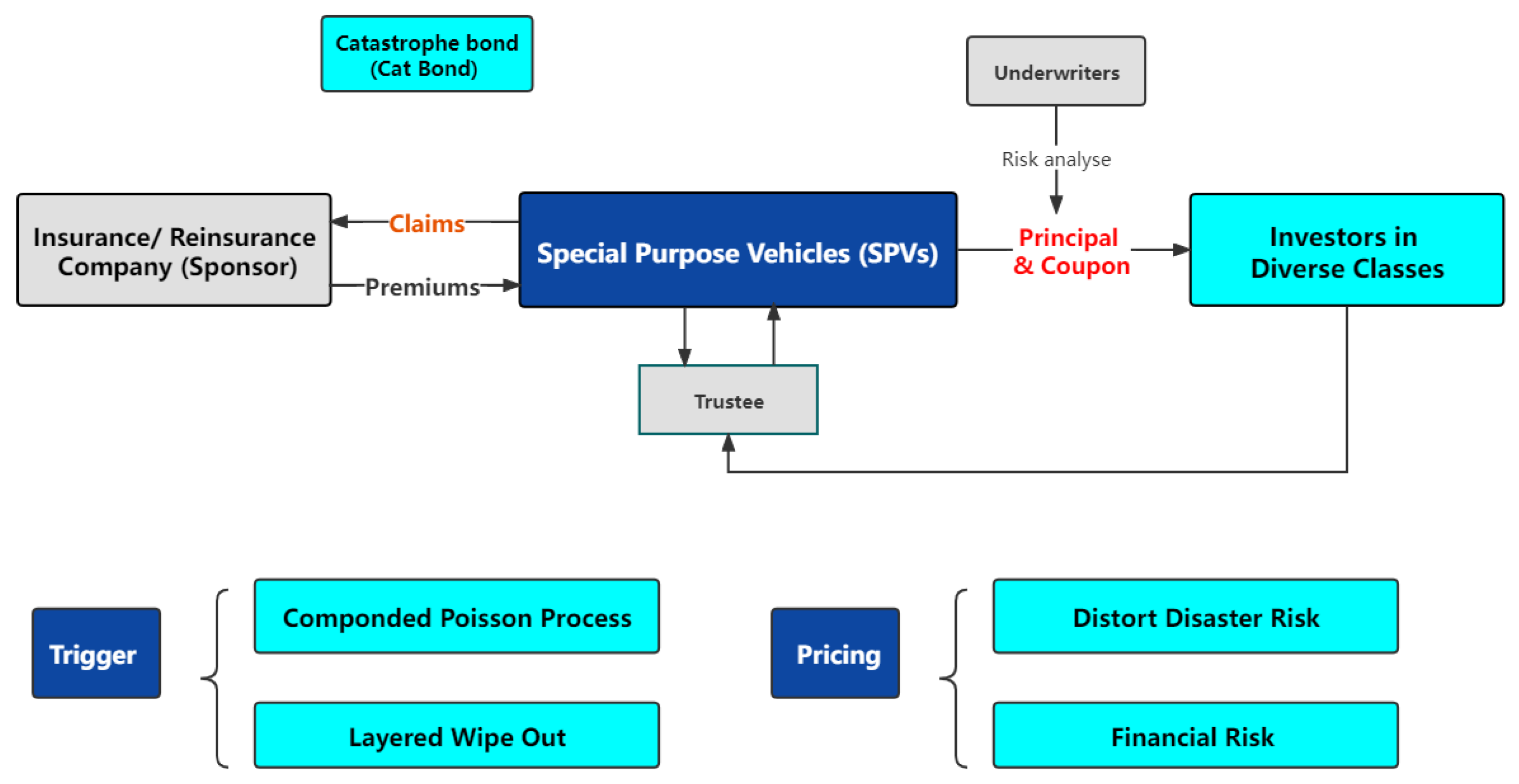
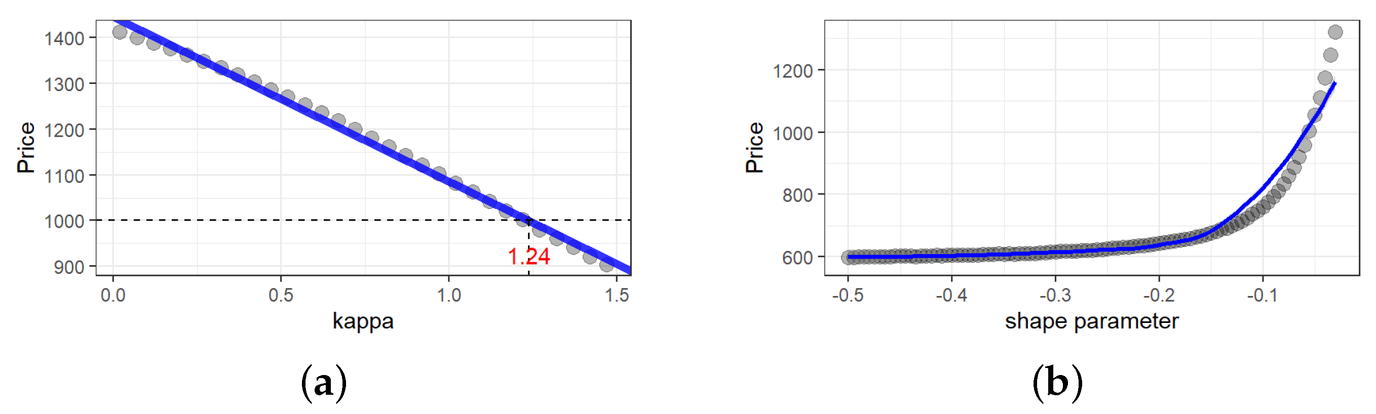
3.2. Design of Flooding Catastrophic Bonds

Trigger selection is of prime importance in the design of CAT bonds. In general, indemnity and nonindemnity triggers constitute the trigger classification. The bases of how they are triggered are the sponsor’s actual loss caused in specified catastrophic occurrences and other quantities for reflecting or approaching the actual loss, e.g., 2015 Acorn Re earthquake CAT bond. This bond was also adopted as the guide for our analysis of the CAT bond triggered by large maximum point precipitation levels. To reconfirm that the maximum point precipitation was a proper trigger choice, we adopted upper tail dependence coefficient (UTDC) and tail quotient correlation coefficient (TQCC) between the maximum point precipitation and economic loss to assist in our discussion. In our calculations, the assumption of the identical and independent distributions of the maximum point precipitation $X_i$ (direct economic losses $Y_i)$ was confirmed by a Ljung–Box test with a p-value of 0.8177 (0.2829). Therefore, the subsequent empirical tail dependence analyses could then be conducted. The empirical u-level tail dependence index is represented as:

$${\chi }_n\left(u\right):=1-\frac{log\mathbb{P}\left\{F_{n1}\left(X_i\right)<u,F_{n2}\left(Y_i\right)<u\right\}}{logu},$$

where $F_{n1}$ and $F_{n2}$ are the empirical marginal distributions of $(X_i,Y_i)$. We see from Figure 4a that ${\chi }_n\left(u\right)$ remains constant for a moderate quantile level. This indicates that large economic losses are likely to occur along with large maximum point precipitation. The tail dependence index $\chi$, as the limit of $\chi \left(u\right)$, was estimated as $2-2^{0.6734}=0.405$, applying a bivariate logistic model for the $90\%$ quantile excess [11]. Meanwhile, we analyzed the relative extremes of the corresponding threshold exceedances with the tail quotient correlation coefficient (TQCC), see, e.g., [12]. Namely,

$$q\left(u\right)=\frac{{max}_{1\le i\le m}\left(\frac{max\left({\tilde{X}}_i,t_u\right)}{max\left({\tilde{Y}}_i,t_u\right)}-1\right)+{max}_{1\le i\le m}\left(\frac{max\left({\tilde{Y}}_i,t_u\right)}{max\left({\tilde{X}}_i,t_u\right)}-1\right)}{{max}_{1\le i\le m}\frac{max\left({\tilde{X}}_i,t_u\right)}{max\left({\tilde{Y}}_i,t_u\right)}\times {max}_{1\le i\le m}\frac{max\left({\tilde{Y}}_i,t_u\right)}{max\left({\tilde{X}}_i,t_u\right)}-1},t_u=-1/logu,u\in (0,1),$$

where $({\tilde{X}}_i,{\tilde{Y}}_i)$ is the unit Fréchet distributed threshold exceedances based on the marginal analysis in Section 2, i.e.,

$${\tilde{X}}_i=-{\left(log\left\{1-{\zeta }_x{\left[1+{\widehat{\xi }}_X\frac{X_i-u_x}{{\widehat{\sigma }}_X}\right]}^{-1/{\xi }_X}\right\}\right)}^{-1},{\tilde{Y}}_i=-{\left(log\left\{1-{\zeta }_Y{\left[1+{\widehat{\xi }}_Y\frac{Y_i-u_Y}{{\widehat{\sigma }}_Y}\right]}^{-1/{\xi }_Y}\right\}\right)}^{-1},$$

where ${\zeta }_X=1-F_X\left(u_X\right)$ and ${\zeta }_Y=1-F_Y\left(u_Y\right)$. We see from Figure 4b that TQCC shows an increasing trend with values apparently larger than 0.1. Therefore, large maximum point precipitation may indicate large economic losses [18]. The naturally arising question for insurers and reinsurers is how to hedge large risk.

The bond market is a logical choice because investors are looking for arbitrage opportunities and can mitigate the loss of insurance products. Collateralized special purpose vehicles (SPVs) issue the CAT bond, which is usually issued and established by sponsors who are insurers and reinsurers. For SPVs, the premium is paid by the sponsor, and reinsurance is used as a return. The incentive premium is usually paid to investors as part of the coupon payment, including the oscillation part related to the national reference interest rate. For example, the London Interbank Offered Rate (LIBOR) and Shanghai Inter-bank Offered Rate (Shibor) can reflect the return from the trust account where the principal is deposited. The principal and coupon payments are reduced whenever a specific triggering event happens. Additionally, sponsors can receive some funds as a repayment for the claims. Here, we followed the product pricing scheme proposed by [3], together with a compound Poisson trigger process similar to the 2015 Acorn Re earthquake CAT bond. The detailed workflow is presented in Figure 5.

Here, we considered a payoff function $\Pi (·)$ and wiped out time $\tau$ defined by

$$\Pi \left(y\right)=max\left\{1-y,0\right\},y\ge 0,\tau =inf\{t\ge 0:\Pi \left(Y_t\right)=0\}.$$

Here, the trigger process $\{Y_t,t\ge 0\}$ was supposed as a compound Poisson trigger process given as

$$\begin{array}{cc}{Y}_t=\hfill & \sum _{j=1}^{N_t}(0.005\times \mathbb{I}\left(X_j\in (803.4,844]\right)+0.01\times \mathbb{I}\left(X_j\in (844,970.89]\right)\hfill \\ \hfill & +0.015\times \mathbb{I}\left(X_j\in (970.89,1247.25]\right)+0.05\times \mathbb{I}\left(X_j\in (1247.25,\infty ]\right)),\hfill \end{array}$$

where $X_j$ denotes the severity of the flooding driver (here, maximum point precipitation), and $N_t$ denotes the number of large maximum point precipitation events up to time t. The four maximum point precipitation levels of 803.4, 844, 970.89, and 1247.25 accounts for the 0.85, 0.9, 0.95, and 0.99 quantiles, respectively, which means when severity is above a certain level of threshold, a fraction $0.5\%,1\%,1.5\%,5\%$ of the principal will be wiped off.

For example, we issue a bond with a face value of 1000 (denoted by K), a maturity of 3 (denoted by T), and a coupon period of 1/4 year (denoted by $\Delta$). The bonds will be paid at $s\Delta$, where $s=1,\dots ,4T$. It follows from Equation (A8) that the price at time t becomes

$$\begin{array}{cc}{P}_t=\hfill & \frac{K}{4}{\mathbb{E}}^{Q^1}\left[\sum _{s=\lfloor t\rfloor +1}^{\lfloor 4\tau \rfloor \wedge 4T}{\mathbb{E}}_t^{Q^2}\left[D(t,s\Delta )\left(R+i_{s\Delta }\right)\Pi \left(Y_{(s-1)\Delta }\right)\right]\right]+K{Q}^1(\tau >T){\mathbb{E}}^{Q^2}[D(t,T)\Pi \left(Y_T\right)]\hfill \\ \hfill & +\frac{K}{4}{\mathbb{E}}^{Q^1}\left[(\tau -\lfloor \tau \rfloor \Delta )\mathbb{I}\left(\tau \le T\right)\Pi \left(Y_{\lfloor \tau \rfloor }\right){\mathbb{E}}^{Q^2}\left[D(t,\tau )\left(R+i_{\tau }\right)\mid \tau \right]\right].\hfill \end{array}$$

(2)

Note that the pricing scheme can only be realized by Monte Carlo simulation. To achieve this, we modeled the maximum point precipitation excess by generalized Pareto distribution $G{P}_{\xi ,\beta }$ following a similar procedure to that used for direct economic losses in Section 3. All the estimates of parameters involved were given in

Table 4. Parameters of interest rate and precipitation modeling.

Panel A: Vasicek models (under ${\mathit{Q}}^2$)
Risk-free rate				Shibor				Correlation
$a_r$	$b_r$	${\sigma }_r$	$r_0$	$a_{\ell }$	$b_{\ell }$	${\sigma }_{\ell }$	${\ell }_0$	$\rho$
1.52	4.12%	1.40%	2.28%	0.04	2.02%	4.00%	2.43%	0.89
Panel B: Maximum point precipitation distribution
Under ${\mathbb{P}}^1$				Under $Q^1$
$\mathbb{P}\left\{X>u\right\}=10\%$				$Q^1(X\le x)=\Phi ({\Phi }^{-1}\left(P^1(X\le x)\right)-\kappa )$
$X-u|(X>u)\sim {\mathrm{GP}}_{\xi ,\beta }$				$\kappa =1.24$
$\xi =-0.0558,\beta =186.6225$
$u=844$
Maximum magnitude: 4187

. We modeled the annual number of maximum point precipitation excess events as a Poisson distribution and obtained an intensity $\lambda$ of 6.94. Furthermore, we implemented Wang’s distortion of disaster risk X [19], i.e.,

$$\tilde{X}=\left[{(1-\Phi ({\Phi }^{-1}\left(U\right)+\kappa ))}^{-\xi }-1\right]\times \frac{\beta }{\xi }+u.$$

Additionally, the financial interest risk $(r_t,{\ell }_t)$ in Equation (A9) was fitted by the 4 years and 3 months China treasury bond rates and 4 years and 3 months Shanghai inter-bank offered rate (Shibor). Estimated parameters were put into the pricing measure that combined a distorted pricing measure representing catastrophe insurance risk and a risk-neutral pricing measure for the arbitrage financial market. The bond price was given by a simulation of ${10}^5$ paths, each with distorted generalized Pareto distributed interarrival time.

Figure 6a shows the price variations in the financial market risk in terms of the distortion parameter $\kappa \in (0,1.5)$ of Wang’s transform. A larger value of $\kappa$ means that investors are exposed to higher risk, so a higher premium will be required, as well as, eventually, a lower bond price. In addition, the practical value of $\kappa =1.24$ was determined when we set the par value $K=1000$ to be equal to the bond price. Furthermore, the sensitivity anylsis was conducted for its shape parameter, presented in Figure 6b. At this time, the ratio of scale $\left(\beta \right)$ to shape $\left(\xi \right)$ was $-3342.863$, which means the maximum (the right endpoint) keeps unchanged at 4186.863. We found that the bond price increased with decreasing shape parameter, which is reasonable in reality as investors are exposed to higher risk and require lower costs/higher returns at this time.

4. Conclusions and Extension Discussions

We determined the marginal tail behaviors of maximum point precipitation events reflecting both the severity of floods in a 24 h rainstorm and its resulting vulnerability risk via the direct economic losses. These findings suggest a compensation mechanism among local, state, and national governments as well as financial markets. Market regulators and investors can utilize our findings for pricing flooding CAT bonds to either mitigate the risk or gain arbitrage according to their real information, e.g., past economic loss, catastrophe frequency, magnitude, and past interest rate. Moreover, they can adjust the price according to their risk attitude or risk tolerance. For instance, pessimistic investors tend to increase the distortion parameter $\kappa$ and increase the absolute value of the shape parameter to mitigate their risk. Otherwise, they may lower these parameters to be actively involved in this market to gain arbitrage. When a market regulator is highly optimistic about the decrease in severity and frequency of a catastrophic event, then the distortion parameter and absolute value of the shape parameter could be lowered and vice versa. Moreover, this pricing framework and implementation of EVT can be adapted to various kinds of catastrophe events including hurricanes, earthquakes, and typhoons [20].

This study lays a foundation for further studies on compound disaster modeling and systemic risk management strategy. In practice, multiple disasters may simultaneously occur or in a chain, e.g., wildfire and air pollution and morbidity from lung-related diseases [21]. Additionally, the regional vulnerability to different natural disasters might be further considered in the future provided that spatial–temporal hydrology data with high enough is available, see, e.g., [22,23] for related studies on spatial modeling of extreme precipitations and grey relational analysis. Given that fine pixel data are available on certain spatial and temporal scales, alternative models of the occurrences of disasters may be applied, including log-Gaussian Cox processes [24] and nonhomogeneous compound Poisson process of the total excess economic losses involved, possibly explained by growing climate change, seasonal clustering factors, as well as different weather types [9]. Finally, the single-trigger CAT bond in this study lays the foundation for multiple-event trigger CAT bonds using the Copula–EVT framework and multiple financial risks including inflation risk (i.e., randomized CPI) and interest risks reflecting economic uncertainty as well [13,25,26].

References

1. Chen, J.; Liu, G.; Yang, L.; Shao, Q.; Wang, H. Pricing and simulation for extreme flood catastrophe bonds. Water Resour. Manag. 2013, 27, 3713–3725. [Google Scholar] [CrossRef]
2. Kundzewicz, Z.W.; Huang, J.; Pinskwar, I.; Su, B.; Szwed, M.; Jiang, T. Climate variability and floods in China—A review. Earth-Sci. Rev. 2020, 211, 103434. [Google Scholar] [CrossRef]
3. Tang, Q.; Yuan, Z. CAT bond pricing: A product probability measure with POT risk characterization. ASTIN Bull. 2019, 49, 457–490. [Google Scholar] [CrossRef] [Green Version]
4. Falk, M.; Hüsler, J.; Reiss, R.D. Extreme Value theory. In Laws of Small Numbers: Extremes and Rare Events; Springer: Basel, Switzerland, 2011; pp. 25–101. [Google Scholar]
5. Cirillo, P.; Taleb, N.N. Tail risk of contagious diseases. Nat. Phys. 2020, 16, 606–613. [Google Scholar] [CrossRef]
6. Embrechts, P.; Klüppelberg, C.; Mikosch, T. Modelling Extremal Events: For insurance and Finance; Springer Science & Business Media: New York, NY, USA, 2013. [Google Scholar]
7. Liu, W.; Wu, J.; Tang, R.; Ye, M.; Yang, J. Daily precipitation threshold for rainstorm and flood disaster in the mainland of China: An economic loss perspective. Sustainability 2020, 12, 407. [Google Scholar] [CrossRef] [Green Version]
8. Towler, E.; Llewellyn, D.; Prein, A.; Gilleland, E. Extreme-value analysis for the characterization of extremes in Water Resources: A generalized workflow and case study on New Mexico monsoon precipitation. Weather Clim. Extrem. 2020, 29, 100260. [Google Scholar] [CrossRef]
9. Aranda, J.A.; García-Bartual, R. Effect of seasonality on the quantiles estimation of maximum floodwater levels in a reservoir and maximum outflows. Water 2020, 12, 519. [Google Scholar] [CrossRef] [Green Version]
10. Sun, R.; Gong, Z.; Gao, G.; Shah, A.A. Comparative analysis of multi-criteria decision-making methods for flood disaster risk in the Yangtze river delta. Int. J. Disaster Risk Reduct. 2020, 51, 101768. [Google Scholar] [CrossRef]
11. Coles, S.; Heffernan, J.; Tawn, J. Dependence measures for extreme value analyses. Extremes 1999, 2, 339–365. [Google Scholar] [CrossRef]
12. Lin, H.; Zhang, Z. Extreme co-movements between infectious disease events and crude oil futures prices: From extreme value analysis perspective. Energy Econ. 2022, 110, 106054. [Google Scholar] [CrossRef]
13. Evgenidis, A.; Tsagkanos, A.; Siriopoulos, C. Towards an asymmetric long-run equilibrium between economic uncertainty and the yield spread. A multi-economy view. Res. Int. Bus. Financ. 2017, 39, 267–279. [Google Scholar] [CrossRef]
14. Surminski, S.; Dorta, D. Flood insurance schemes and climate adaptation in developing countries. Int. J. Disaster Risk Reduct. 2014, 7, 154–164. [Google Scholar] [CrossRef] [Green Version]
15. Loretan, M.; Philips, P.C.B. Testing the covariance stationarity of heavy tailed time series: An overview of the theory with applications to several financial datasets. J. R. Stat. Soc. 1994, 1, 211–248. [Google Scholar] [CrossRef]
16. Coles, S. An Introduction to Statistical Modeling of Extreme Values; Springer Series in Statistics; Springer: London, UK, 2001. [Google Scholar]
17. Scarrott, C.; MacDonald, A. A review of extreme value threshold estimation and uncertainty quantification. Rev. Stat. J. 2021, 10, 33–60. [Google Scholar]
18. Zhao, Y.; Gong, Z.; Wang, W.; Luo, K. The comprehensive risk evaluation on rainstorm and flood disaster losses in China mainland from 2004 to 2009: Based on the triangular grey correlation theory. Nat. Hazards 2014, 71, 1001–1016. [Google Scholar] [CrossRef]
19. Wang, S.S. A class of distortion operators for pricing financial and insurance risks. J. Risk Insur. 2000, 67, 15–36. [Google Scholar] [CrossRef] [Green Version]
20. Shao, J.; Pantelous, A.; Papaioannou, A.D. Catastrophe risk bonds with applications to earthquakes. Eur. Actuar. J. 2015, 5, 113–138. [Google Scholar] [CrossRef]
21. Cui, P.; Peng, J.; Shi, P.; Tang, H.; Ouyang, C.; Zou, Q.; Liu, Q.; Lei, Y. Scientific challenges of research on natural hazards and disaster risk. Geogr. Sustain. 2021, 2, 216–223. [Google Scholar] [CrossRef]
22. Ho, C.T. Measuring bank operations performance: An approach based on grey relation analysis. J. Oper. Res. Soc. 2006, 57, 337–349. [Google Scholar] [CrossRef]
23. Alston, A. A Bayesian Spatial Analysis of Extreme Precipitation. Ph.D. Thesis, North Carolina State University, Raleigh, NC, USA, 2011. [Google Scholar]
24. Koh, J.; Pimont, F.; Dupuy, J.L.; Opitz, T. Spatiotemporal wildfire modeling through point processes with moderate and extreme marks. arXiv 2021, arXiv:2105.08004. [Google Scholar]
25. Ibrahim, R.A.; Napitupulu, H. Multiple-trigger catastrophe bond pricing model and its simulation using numerical methods. Mathematics 2022, 10, 1363. [Google Scholar] [CrossRef]
26. Wei, L.; Liu, L.; Hou, J. Pricing hybrid-triggered catastrophe bonds based on copula-EVT model. Quant. Financ. Econ. 2022, 6, 223–243. [Google Scholar] [CrossRef]
27. Gilleland, E.; Katz, R.W. Extremes 2.0: An extreme value analysis package in R. J. Stat. Softw. 2016, 72, 1–39. [Google Scholar] [CrossRef] [Green Version]
28. Wang, R.; Wei, Y. Characterizing optimal allocations in quantile-based risk sharing. Insur. Math. Econ. 2020, 93, 288–300. [Google Scholar] [CrossRef]
29. Mamon, R.S. Three ways to solve for bond prices in the Vasicek model. J. Appl. Math. Decis. Sci. 2004, 8, 1–14. [Google Scholar] [CrossRef]
Figure 1. Workflow of flooding risk management.
Mathematics 11 00114 g001
Figure 2. Histogram of (a) economic loss and (b) maximum point precipitation, and (c) scatter plot of economic loss in billion yuan on log scale against maximum point precipitation in millimeters.
Mathematics 11 00114 g002
Figure 3. (a) Sample mean excess for economic loss in billion yuan with grey dash line representing 95% confidence interval. (b) Variation plots of location, scale, and shape (from top to bottom) against threshold u ( 1.5 , 5 ) .
Mathematics 11 00114 g003
Figure 4. The empirical tail dependence measures (a) the Chi plot χ n ( u ) and (b) the tail quotient correlation coefficient q ( u ) . The solid lines and dotted lines show the estimate and 95% pointwise confidence intervals, respectively. The estimate of the tail dependence index χ ^ = 2 2 0.6734 = 0.405 is indicated by the horizontal line using the bivariate logistic extreme value model.
Mathematics 11 00114 g004
Figure 5. Operation mechanism for catastrophe bonds.
Mathematics 11 00114 g005
Figure 6. The empirical price at t = 0 varies with (a) the distortion parameter κ and (b) the shape parameter ξ with β / ξ = −3342, κ = 1.24 . Here, the empirical price is given by Equation (2) and a simulation of 10 5 samples of the threshold excess of maximum point precipitation from GP ξ , β , with all other parameters specified in Table 4.
Mathematics 11 00114 g006