Tail Risk Signal Detection through a Novel EGB2 Option Pricing Model

Abstract

Connecting derivative pricing with tail risk management has become urgent for financial practice and academia. This paper proposes a novel option pricing model based on the exponential generalized beta of the second kind (EGB2) distribution. The newly proposed model is of generality, simplicity, robustness, and financial interpretability. Most importantly, one can detect tail risk signals by calibrating the proposed model. The model includes the seminal Black–Scholes (B−S) formula as a limit case and can perfectly “replicate” the option prices from Merton’s jump-diffusion model. Based on the proposed pricing model, three tail risk warning measures are introduced for tail risk signals detection: the EGB2 implied tail index, the EGB2 implied Value-at-Risk (EGB2-VaR), and the EGB2 implied risk-neutral density (EGB2 R.N.D.). Empirical results show that the new pricing model can yield higher pricing accuracy than existing models in normal and crisis periods, and three model-based tail risk measures can perfectly detect tail risk signals before financial crises.

1. Introduction

The latest empirical research studies have shown that financial asset returns are asymmetrically distributed and information regarding tail risks are missing when using conventional Gaussian type asset pricing formulas [1,2]. For example, investors underestimate left tail risk and under-insure against very low oil prices in crude oil derivative markets [2]. Motivated by the leptokurtic feature of asset returns and excessive losses caused by financial crises, the literature began to link tail risk management with derivative pricing [3,4,5]. In this regard, option-trading-based strategies were introduced, and novel options were designed for tail risk hedging. Meanwhile, several non-Gaussian distributions were adopted for revising conventional option pricing models.

Next, we first start to give a brief review of tail risk hedging and existing option pricing models dealing with tail risks and leptokurtic features, and then discuss the practical limitations and design insufficiency of those pricing models closely related to our proposed work in this paper.

Regarding tail risk hedging using options, the seminal works were due to Bhansali (2008, 2014) [6,7], providing a valuable benchmark for developing option-based tail risk hedging strategies. Based on their framework, offensive tail risk management [8], active tail risk management [9], behavioral insight [10], tail risk hedging in a low-rate environment [11], and hedging robustness during extreme events such as COVID-19 [12] were further investigated. Furthermore, novel options were also designed for tail risk hedging purposes [13].

For the leptokurtic features, extreme losses and fat-tail phenomena were considered by using non-Gaussian distributions to model underlying asset returns in option pricing models. The typical distributions include: (1) generalized distributions, such as GB class [14,15,16], generalized extreme value (GEV) [17], and generalized logistic (GLO) [18]; (2) asymmetric distributions, such as skewed-t [19], variance gamma [20], Weibull [21], and distorted lognormal distribution [22]; and (3) mixture distribution such as the mixture of Gaussian and heavy-tailed model [23].

To detect tail risk signals via an option pricing model, a natural choice for the underlying asset’s modeling is GEV distribution. In this regard, Markose and Alentorn (2011) [17] proposed a GEV option pricing model, from which one can obtain implied volatility and implied tail index simultaneously by using option price data. However, empirical study shows that the GEV pricing model did not perform well during many time periods (Kim and Kim, 2014 [18]). One reason may be that using the GEV to fit losses could cause the over-fitting problem. According to Fisher–Tippett theorem [24], it is the block maxima of returns and/or losses rather than returns and/or losses per se that follow the GEV distribution. This is the so-called “domain of attraction” principle, based on which it is to conclude that directly pre-assuming the daily losses to be a GEV distribution may not be either mathematically or practically reasonable (in the empirical result of Markose and Alentorn (2011) [17], the implied tail indexes vary from positive to negative back and forth frequently, which may also imply the GEV setting can be questionable, thereby making their results suffering an over-fitting problem in some market circumstances).

Besides the GEV distribution, attention was also paid to the GB class distributions. In particular, the generalized beta of the second kind (GB2) and the exponential generalized beta of the second kind (EGB2) distributions show promising potential. For example, McDonald and Bookstaber (1991) [14] proposed a GB2 option pricing model in the literature. Based on the equilibrium conditions proposed by Cox and Ross (1976) [25], the GB2 option pricing model can obtain a closed-form solution by using GB2 cumulative distribution function (C.D.F.). However, in the explicit expression of the theoretical option prices, there exists a term $S_T$, which means that the theoretical option prices can only be determined when the underlying asset price at the maturity date T is known; but, such an assumption is practically not implementable. The reason is, based on the payoff functions of vanilla options, if $S_T$ is given, the option prices are known, which means that we do not need additional information or a pricing formula in this case. In addition, Fischer (2000) [17] proposed an Esscher-EGB2 option pricing model, where the underlying price process is modeled by an exponential EGB2-Lévy motion. By using the Esscher transformation, pricing formulas are given. There are some problems with the formula in practice. The final expression of the pricing model involves a Fourier inversion formula. Moreover, it is composed of complex numbers, meaning one must implement numerical methods to obtain the theoretical prices. In the pricing and risk management realms, the numerical method makes the pricing formula relatively complicated and less feasible. Another GB2 pricing model was proposed by Mirfendereski and Rebonato (2001) [16], which has a straightforward closed-form pricing formula. However, one essential assumption of “zero risk-free rate” makes the model not applicable in the non-zero rate real world.

Whereas the existing studies do provide a valuable basis for related research, we note that there are still many gaps in this field. First, many of the non-Gaussian option pricing models can be too “ad hoc” to be applicable in the real world. By merely focusing on specific market situations or strongly relying on “too-strong” pre-assumptions, one may lose the feasibility and generality of the pricing models, thereby making it of less pricing accuracy and robustness. In addition, we note that many existing non-Gaussian option pricing models do not entail the benchmark Black–Scholes (B−S) model [26] or any Gaussian models as special cases, which also hinders the models’ universality and financial interpretability. Second, many existing models may suffer from simplicity and feasibility issues. For instance, the model based on the Lévy process may include complex numbers in its resulting formula, which means that one has to use numerical methods to obtain theoretical option prices. Meanwhile, the models that adopt time-changed motions or jump-diffusion processes are mathematically complicated, which may add lots of computational burdens and difficulties in practice. Last but not least, most of the existing research mainly paid attention to the pricing but rarely discussed the connection with risk analysis. For example, in the seminal B−S formula, one can “detect” the overall market risk level by directly looking at the option price and calculating the corresponding B−S implied volatility. However, similar discussions are relatively scarce for non-Gaussian distribution-based models.

This paper proposes a novel option pricing model based on the exponential generalized beta of the second kind (EGB2) distribution, which fills the current gaps by introducing the following novelties. First, the newly proposed EGB2 option pricing (EGB2OP) model is of great generality, interpretability, and robustness. It contains the seminal B−S model as a limit case and can replicate option prices generated from the jump-diffusion model, thereby making it robust in varying market seniors. The resulting pricing formulas are analog to the form of the B−S model while providing additional financial interpretability for each parameter (See Section 3.3). With a B−S analogous pricing formula, the newly proposed model preserves the B−S model’s interpretability characteristics and adds capacity for characterizing the tail behavior and asymmetry in price changes. Second, the proposed model is of great simplicity. It does not include complex numbers, “too-strong” pre-assumptions, or complicated mathematical processes, thereby making it computationally cheaper. This may offer an attractive competitive advantage in terms of practical utilization. Finally, based on the proposed model, tail risk signals can be directly detected or “implied” from option prices. Based on our pricing model, we propose three model-based risk measures, which may offer powerful implications for both investors and policymakers. Just like one can “detect” the overall market risk signal via the B−S formula by looking at the implied volatility, people can directly “detect” the tail risk signal via the EGB2OP model by looking at the implied tail index. To the authors’ best knowledge, to date, there is no model equivalent to the one proposed by this paper. It is worth noting that the reason why our EGB2OP model is of generality, robustness, and satisfactory pricing and risk reporting performances is not because it includes more than one parameter, but because of the interpretable structure of the model per se. As a matter of fact, as reviewed before, there are many option pricing models in the literature having many or even more parameters, and they may not be able to obtain satisfactory properties.

The rest of the paper is organized as follows. Section 2 provides a brief review of the EGB2 distribution. The EGB2OP model is proposed in Section 3. Section 4 provides the simulation experiments that compare the pricing performance and flexibility of the B−S model and EGB2OP model. Section 5 uses simulation examples to examine the ability of the EGB2OP model to “replicate” Merton’s jump-diffusion model and compare their pricing performances under various market scenarios. Section 6 provides the empirical results using China’s option market data. Three EGB2OP model-based measures are designed for detecting tail risk signals in Section 7. Section 8 concludes the paper. Additional derivations and examples are presented in the Appendix A.

2. Review of the EGB2 Distribution

The exponential generalized beta of the second kind (EGB2) distribution is proposed by McDonald and Xu (1995) [27], which is a generalization of both logistic distribution and beta distribution. The standardized density function (with neither location parameter nor scale parameter) of EGB2 is given by Equation (1):

$$f(x;p,q)=\frac{exp\left(px\right)}{B(p,q){[1+exp\left(x\right)]}^{p+q}},x\in \mathbb{R}$$

(1)

where $B(·,·)$ is an incomplete beta function, and $p>0$ and $q>0$ are shape parameters or tail parameters governing the left tail and right tail of the distribution, respectively. Introducing location parameter a and scale parameter $b>0$ leads to a four parameters p.d.f. as Equation (2):

$$f(x;a,b,p,q)=\frac{exp\left(p\frac{x-a}{b}\right)}{bB(p,q){[1+exp\left(\frac{x-a}{b}\right)]}^{p+q}},x\in \mathbb{R},$$

(2)

and denote its corresponding distribution function as EGB2($x;a,b,p,q$) or EGB2($a,b,p,q$) for a short notation. When $a=0$ and $b=1$, it is denoted as EGB2($x;p,q$).

Tail Parameters and Tail Behavior. According to McDonald (1991) [28], the relative gap between the left tail parameter p and the right tail parameter q has essential meaning for capturing tails’ behavior. If $p>q$, the distribution is positively skewed. If $p<q$, the distribution is negatively skewed. If $p=q$, the distribution is symmetric. In general, the smaller the value of q, the more the distribution is skewed to the right; the smaller the value of p, the more the distribution is skewed to the left. In the empirical literature, it has been shown that the extreme behaviors of asset returns (losses) are highly asymmetrical, especially during extreme events [29]. Thus, it would be of practical significance to trace tail behaviors on both tails.

Special Cases. According to McDonald and Xu (1995) [27], EGB2 goes in limit to Weibull when $p\to 1$ and $q\to \infty$, to standard logistic when $p=q=1$, to EGG or lognormal when $q\to \infty$, to BR2 or EBR2 when $p=1$, and to normal when $p\to \infty$ and $q\to \infty$. To see more special cases for EGB2, refer to the partial EGB distribution tree by McDonald and Xu (1995) [27].

The Moments. In the literature [27,28,30], the characteristic function and moment-generating function of X are given by

$${\phi }_X\left(t\right)=M_X\left(it\right)=exp\left(at\right)\frac{B(p+bit,q-bit)}{B(p,q)}=exp\left(at\right)\frac{\Gamma (p+bit,q-bit)}{\Gamma (p,q)},$$

(3)

and

$$M_X\left(t\right)=exp\left(at\right)\frac{B(p+bt,q-bt)}{B(p,q)},-p<bt<q,$$

(4)

respectively, from which we can obtain the moments of the EGB2 distributions.

The first moment of EGB2 is

$$M_1=E\left(X\right)=a+b[\phi \left(p\right)-\phi \left(q\right)],$$

(5)

where $\phi (·)$ is the digamma function, given by

$$\phi \left(x\right)=\frac{\mathrm{d}ln[\Gamma (x\left)\right]}{\mathrm{d}x}=\frac{{\Gamma }^{\prime }\left(x\right)}{\Gamma \left(x\right)}.$$

The second to fourth moments of EGB2 are

$$M_2=Var\left(X\right)=b^2[{\phi }^{\prime }\left(p\right)+{\phi }^{\prime }\left(q\right)],$$

(6)

$$M_3=b^3[{\phi }^{\prime \prime }\left(p\right)-{\phi }^{\prime \prime }\left(q\right)],$$

(7)

$$M_4=b^4[{\phi }^{\prime \prime \prime }\left(p\right)+{\phi }^{\prime \prime \prime }\left(q\right)+3{[{\phi }^{\prime }\left(p\right)+{\phi }^{\prime }\left(q\right)]}^2].$$

(8)

To further capture the tail behavior, one can define the standardized third (skewness) and fourth (kurtosis) moments as:

$$S\left(X\right)=\frac{M_3}{M_2^{3/2}}=\frac{{\phi }^{\prime \prime }\left(p\right)-{\phi }^{\prime \prime }\left(q\right)}{{[{\phi }^{\prime }\left(p\right)+{\phi }^{\prime }\left(q\right)]}^{3/2}},$$

(9)

$$K\left(X\right)=\frac{M_4}{M_2^{4/2}}=\frac{{\phi }^{\prime \prime \prime }\left(p\right)+{\phi }^{\prime \prime \prime }\left(q\right)+3{[{\phi }^{\prime }\left(p\right)+{\phi }^{\prime }\left(q\right)]}^2}{{[{\phi }^{\prime }\left(p\right)+{\phi }^{\prime }\left(q\right)]}^2}.$$

(10)

These quantities will be used in the subsequent computations.

The Relationship with GB2 [27,31]. Compared to the conventional relationship between normal and lognormal, the EGB2 distribution has a similar connection to the generalized beta of the second kind (GB2) distribution. If $X\sim GB2(a,b,p,q)$, then the variable $Y=log\left(X\right)\sim EGB2(a,b,p,q)$.

In the literature, EGB2 distribution has been widely used in empirical studies, such as the modeling of income distribution [27], stock returns [32], future markets’ sentiment [33], currency exchange rates [34,35], and carbon emission inequality [36].

3. Derivations of the EGB2 Option Pricing Model

3.1. The EGB2 Option Pricing Model for Calls

According to Harrison and Pliska (1981) [37], the equilibrium European call option price can be written as:

$$C_t\left(K\right)=e^{-r(T-t)}{\int }_K^{\infty }(S_T-K)g\left(S_T\right)d{S}_T,$$

(11)

where r is a risk free rate parameter, $g(.)$ is the pricing kernel, t is the present time, T is the time at maturity, $S_T$ is the underlying stock/asset price at time T.

We start from (11) to derive our new EGB2 option pricing formula. Define the negative log-returns of the underlying asset over time interval $[t,T]$ as follows:

$$L_{t,T}=ln\left(S_t\right)-ln\left(S_T\right)\sim EGB2(a_{t,T},b_{t,T},p_{t,T},q_{t,T}),$$

i.e., the density function for losses is given by:

$$f\left(L_{t,T}\right)=\frac{exp\left(p\frac{L_{t,T}-a_{t,T}}{b_{t,T}}\right)}{b_{t,T}B(p_{t,T},q_{t,T}){[1+exp\left(\frac{L_{t,T}-a_{t,T}}{b_{t,T}}\right)]}^{p_{t,T}+q_{t,T}}}.$$

(12)

Since

$$\left|\frac{\partial L_{t,T}}{\partial S_T}\right|=\left|-\frac{1}{S_T}\right|=\frac{1}{S_T},$$

the risk-neutral density (R.N.D.) for underlying price at time T is given by:

$$g\left(S_T\right)=\left|\frac{\partial L_{t,T}}{\partial S_T}\right|f\left(L_{t,T}\right)=\frac{exp\left(p\frac{L_T-a_{t,T}}{b_{t,T}}\right)}{b_{t,T}{S}_{T}B(p_{t,T},q_{t,T}){[1+exp\left(\frac{L_{t,T}-a_{t,T}}{b_{t,T}}\right)]}^{p_{t,T}+q_{t,T}}}.$$

(13)

Inserting Equation (13) into (11), we have

$$C_t\left(K\right)=e^{-r(T-t)}{\int }_K^{\infty }(1-K/S_T)\frac{exp\left(p\frac{L_{t,T}-a_{t,T}}{b_{t,T}}\right)}{b_{t,T}B(p_{t,T},q_{t,T}){[1+exp\left(\frac{L_{t,T}-a_{t,T}}{b_{t,T}}\right)]}^{p_{t,T}+q_{t,T}}}d{S}_T.$$

(14)

By changing the variable, let

$$\gamma =\frac{L_{t,T}-a_{t,T}}{b_{t,T}}=\frac{ln(S_t/S_T)-a_{t,T}}{b_{t,T}},$$

(15)

then the upper bound of the integral in Equation (14) becomes $-\infty$ and the lower bound of the integral becomes

$$H=\frac{ln(S_t/K)-a_{t,T}}{b_{t,T}}$$

and

$$d\gamma =-\frac{1}{b_{t,T}{S}_T}d{S}_T,$$

i.e.,

$$d{S}_T=-b_{t,T}{S}_{T}d\gamma ,$$

and by Equation (15) we have

$$S_T=-S_t{e}^{-a_{t,T}-b_{t,T}\gamma }.$$

Then, Equation (14) becomes

$$C_t\left(K\right)=e^{-r(T-t)}{\int }_{-\infty }^H(S_T-K)\frac{exp\left(p_{t,T}\gamma \right)}{B(p_{t,T},q_{t,T}){[1+exp\left(\gamma \right)]}^{p_{t,T}+q_{t,T}}}d\gamma .$$

(16)

We have

$$\begin{array}{cc}\hfill & {\int }_{-\infty }^H{S}_T\frac{exp\left(p_{t,T}\gamma \right)}{B(p_{t,T},q_{t,T}){[1+exp\left(\gamma \right)]}^{p_{t,T}+q_{t,T}}}d\gamma \hfill \\ \hfill =& S_t{e}^{-a_{t,T}}{\int }_{-\infty }^H\frac{exp\left((p_{t,T}-b_{t,T})\gamma \right)}{B(p_{t,T},q_{t,T}){[1+exp\left(\gamma \right)]}^{p_{t,T}+q_{t,T}}}d\gamma \hfill \\ \hfill =& S_t{e}^{-a_{t,T}}\frac{B(p_{t,T}-b_{t,T},q_{t,T}+b_{t,T})}{B(p_{t,T},q_{t,T})}\hfill \\ \hfill & ·{\int }_{-\infty }^H\frac{exp\left((p_{t,T}-b_{t,T})\gamma \right)}{B(p_{t,T}-b_{t,T},q_{t,T}+b_{t,T}){[1+exp\left(\gamma \right)]}^{(p_{t,T}-b_{t,T})+(q_{t,T}+b_{t,T})}}d\gamma \hfill \\ \hfill =& S_t{e}^{-a_{t,T}}\frac{B(p_{t,T}-b_{t,T},q_{t,T}+b_{t,T})}{B(p_{t,T},q_{t,T})}EGB2(H;p_{t,T}-b_{t,T},q_{t,T}+b_{t,T}),\hfill \end{array}$$

(17)

where $p_{t,T}>b_{t,T}$ has to be satisfied to guarantee the input of beta function is positive (in real data, this condition is almost always satisfied. See Section 5).

Inserting Equations (17) into (15), we obtain a closed form for the EGB2 call option price:

$$\begin{array}{cc}\hfill C_t\left(K\right)=& S_t{e}^{-a_{t,T}-r(T-t)}\frac{B(p_{t,T}-b_{t,T},q_{t,T}+b_{t,T})}{B(p_{t,T},q_{t,T})}EGB2(H;p_{t,T}-b_{t,T},q_{t,T}+b_{t,T})\hfill \\ \hfill & -K{e}^{-r(T-t)}EGB2(H;p_{t,T},q_{t,T}).\hfill \end{array}$$

(18)

Denote that

$$G_1=EGB2(H;p_{t,T}-b_{t,T},q_{t,T}+b_{t,T}),$$

$$G_2=EGB2(H;p_{t,T},q_{t,T}),$$

and

$$B=\frac{B(p_{t,T}-b_{t,T},q_{t,T}+b_{t,T})}{B(p_{t,T},q_{t,T})},$$

the Equation (18) can be simplified as

$$C_t\left(K\right)=S_t{e}^{-a_{t,T}-r(T-t)}B·G_1-K{e}^{-r(T-t)}{G}_2,$$

(19)

which is the EGB2OP formula for the European call option.

3.2. The EGB2 Option Pricing Model for Puts

Starting from the put option formula from Harrison and Pliska (1981) [37], and then following the same lines of derivations in Section 3.1, we can obtain a closed-form formula for EGB2 put option price as

$$\begin{array}{cc}\hfill P_t\left(K\right)=& K{e}^{-r(T-t)}[1-EGB2(H;p_{t,T},q_{t,T})]\hfill \\ \hfill -& S_t{e}^{-a_{t,T}-r(T-t)}\frac{B(p_{t,T}-b_{t,T},q_{t,T}+b_{t,T})}{B(p_{t,T},q_{t,T})}[1-EGB2(H;p_{t,T}-b_{t,T},q_{t,T}+b_{t,T})].\hfill \end{array}$$

(20)

Denote

$$G_3=1-EGB2(H;p_{t,T},q_{t,T}),$$

$$G_4=1-EGB2(H;p_{t,T}-b_{t,T},q_{t,T}+b_{t,T}),$$

then the put option pricing formula can be expressed as

$$P_t\left(K\right)=K{e}^{-r(T-t)}{G}_3-S_t{e}^{-a_{t,T}-r(T-t)}B·G_4.$$

(21)

3.3. The B−S Model as Limit Cases of the EGB2 Option Pricing Model

According to McDonald and Xu (1995) [27], when $p,q\to \infty$, the EGB2 density $f(x;a,b,p,q)$ in (2) has the following limit (for convenience, the time subscript of each EGB2 parameter is omitted in this subsection):

$$f(x;a,b,p,q)\to f_N(x;a,b),$$

where the limit $f_N(x;a,b)=\frac{1}{\sqrt{2\pi b^2}}exp(-\frac{{(x-a)}^2}{2b^2})$ is a normal p.d.f with the location and scale parameter being a and b, respectively.

To connect the B−S pricing model to the EGB2OP model, we consider taking $a=a_{p,q}^{(\delta ,b)}$ such that

$$a_{p,q}^{(\delta ,b)}=-ln\frac{EGB2(H_{p,q}^{(\delta ,b)}+(b+\delta );p-b,q+b)}{EGB2(H_{p,q}^{(\delta ,b)};p,q)}-r(T-t)+ln\frac{B(p-b,q+b)}{B(p,q)},$$

(22)

where $H_{p,q}^{(\delta ,b)}=log(S_t/K)-a_{p,q}^{(\delta ,b)})/b$, and $\delta$ is a tuning parameter for (22) to hold. (18) can then be expressed as

$$\begin{array}{cc}\hfill C_{t,p,q}^{\delta }\left(K\right)=& S_{t}EGB2(H_{p,q}^{(\delta ,b)}+(b+\delta );p-b,q+b)\hfill \\ \hfill & -K{e}^{-r(T-t)}EGB2(H_{p,q}^{(\delta ,b)};p,q).\hfill \end{array}$$

(23)

We now consider the limit of (22) and (23). Set $q/p\to C_1$ when $p\to \infty ,q\to \infty$. When $C_1=1$, EGB2 is symmetric in both tails, i.e., both p and q are large. It is easy to see that the limits of $EGB2(H;p-b,q+b)$ and $EGB2(H;p,q)$ are $N\left(H\right)$, where $N(·)$ is the cumulative distribution function (C.D.F.) of the standard normal distribution. Using Stirling’s approximation, we can prove that $\frac{B(p-b,q+b)}{B(p,q)}$ tends to $C_1^b$ when $p\to \infty ,q\to \infty$.

For $b>0$ and a suitable choice of $\delta$, taking $a=a^{(\delta ,b)}$ such that

$$a^{(\delta ,b)}=-ln\frac{N(H^{(\delta ,b)}+(b+\delta ))}{N\left(H^{(\delta ,b)}\right)}-r(T-t)+bln\left(C_1\right),$$

(24)

where $H^{(\delta ,b)}=(log(S_t/K)-a^{(\delta ,b)})/b$. It is apparent that the right-hand side of (24) is the limit case of (22), and the existences of $a^{(\delta ,b)}$ and $\delta$ are easy to check. Suppose $q/p\to C_1$ when $p\to \infty ,q\to \infty$. The call price formula $C_t\left(K\right)$ in (18) has the following limit:

$$C_t^{\left(\delta \right)}\left(K\right)=S_{t}N(H^{(\delta ,b)}+(b+\delta ))-K{e}^{-r(T-t)}N\left(H^{(\delta ,b)}\right).$$

(25)

Recall that the B−S formula has the following expression:

$$C_t^{BS}\left(K\right)=S_{t}N\left(d_1\right)-K{e}^{-r(T-t)}N\left(d_2\right)$$

(26)

with $d_2=\frac{ln(S_t/K)+r(T-t)-\frac{1}{2}{\sigma }^2(T-t)}{\sigma \sqrt{T-t}}$ and $d_1=\frac{ln(S_t/K)+r(T-t)+\frac{1}{2}{\sigma }^2(T-t)}{\sigma \sqrt{T-t}}=d_2+\sigma \sqrt{T-t}$.

We have the following Theorem 1.

Theorem 1. 

For any given r, σ, $S_t$, T, and K, suppose there exists a $C_1$ as the limit of $q/p$ when $p\to \infty ,q\to \infty$. Then, there exist $a^{(\delta ,b)},b>0,\delta$ satisfy the following two equations:

$$\begin{array}{cc}\hfill b+\delta & =\sigma \sqrt{T-t},\hfill \\ \hfill H^{(\delta ,b)}& =\frac{ln(S_t/K)+r(T-t)-\frac{1}{2}{\sigma }^2(T-t)}{\sigma \sqrt{T-t}},\hfill \end{array}$$

(27)

and Equation (24), and furthermore (25) and (26) are equivalent.

The proof of Theorem 1 is by solving a system of linear equations in (27) and (24) to determine $C_1$. From Theorem 1, we can conclude that the B−S formula $C_t^{BS}\left(K\right)$ is a special case of $C_t^{\left(\delta \right)}\left(K\right)$, which is a special limit class of the EGB2OP call price $C_t\left(K\right)$ in (18) under the condition (27). Then, it is clear that the EGB2OP call price $C_t\left(K\right)$ in (18) covers a much wider range of prices than the B−S formula $C_t^{BS}\left(K\right)$, and it is a much more flexible pricing formula than the B−S formula. A comparison in Figure 1 and empirical studies and an event study further confirm this claim. In Figure 1, we plot the B−S prices and the limit EGB2OP prices $C_t^{\left(\delta \right)}\left(K\right)$ on three options’ moneyness types: at-the-money (ATM, $S_t=K=5$), in-the-money (ITM, $S_t=5.5,K=5$), and out-of-the-money (OTM, $S_t=4.5,K=5$) with varying b values. In each panel, the EGB2OP prices are computed by $\delta$ ranging from 0.1 to 0.9 by a step size of 0.01. Without loss of generality, we set $T-t=1$ and $r=0.03$. The figure reveals that the B−S call prices are within the range of the $C_t^{\left(\delta \right)}\left(K\right)$. As a result, the B−S call prices can be approximated by an EGP2OP model with the optimal choices of $a,b,p,q$.

For all moneyness types, given $\delta$, $C_t^{\left(\delta \right)}\left(K\right)$ and the B−S price are both increasing functions of b. This can be intuitively explained by the fact that b is the scale parameter. Larger values in b imply a greater risk of the underlying asset, and thus the increased expense of the option. Given H and b, the EGB2OP limit price $C_t^{\left(\delta \right)}\left(K\right)$ is monotonically increasing in $\delta$. Among them, there exists one $\delta$ satisfying that $C_t^{\left(\delta \right)}\left(K\right)=C_t^{BS}\left(K\right)$. This interesting result reveals the EGB2OP model’s ability to price a wide range of options. Meanwhile, as can be seen from the Figure 1, the B−S price lines are almost always right in the middle of the corresponding EGB2 prices belt for each case, which gives a sense that the EGB2OP price indeed goes to a limit of the B−S price. This is an intuitive illustration of Theorem 1.

Similarly, using the same arguments of call options, we show that the B−S formula for puts is a limit case of the EGB2OP model for puts.

For the limit cases above, we add the following two additional interpretations and remarks. Considering that a is a location parameter, it means that there can be a price shift in the EGB2OP model compared with the B−S model. In (26), b can be interpreted as the volatility $\sigma$ in the classical B−S call options formula. Borrowing the idea from Mirfendereski and Rebonato (2001) [16] we can derive a so-called “equivalent volatility” of the EGB2OP model by computing

$${\sigma }_{equivalent}=\frac{b}{\sqrt{T-t}}.$$

However, it does not make any comparable sense because the “equivalent volatility” is only “equivalent” to the B−S implied volatility in the limit case, i.e., if and only if p and q tend to infinity simultaneously. Otherwise, one should take not only the value of a and b but also p and q into consideration so as to calculate the standard deviation of the underlying return distribution. In real data, the calibrated p and q typically range from 0.5 to 3.5 and seldom go above 10. Therefore, computing ${\sigma }_{equivalent}$ and comparing it with the B−S implied volatility regardless of the finite (and often not large) value of tail parameters p and q is reckless and meaningless. For comparison purposes, one should compute the standard deviation of underlying return distribution by calibrating EGB2OP models (see Section 6.3).

$B=\frac{B(p-b,q+b)}{B(p,q)}$ indicates the changing of numeraire. Compared to the intuition behind the B−S model, the term $B=\frac{B(p-b,q+b)}{B(p,q)}$ is used to change the numeraire from a riskless bond into an underlying risky asset. In the EGB2OP Formulas (19) and (21), $B·G_1$ and $B·G_4$ are EGB2 probabilities based on underlying risky asset as numeraire, and $G_2$ and $B·G_3$ are EGB2 probabilities based on riskless bond.

4. Simulation Study: Comparison of the EGB2OP Model and the B−S Model

To highlight the flexibility of the EGB2OP model and the fact that the B−S model can be a particular limit case of the EGB2OP model, we simulate option prices with one of the pricing models and approximate the prices with the other one. We examine the pricing accuracy by computing RMSE and MAE for each case. To illustrate the difference between the approximations and the simulated prices, we show Price to Price plots (p-p plots, simulated benchmark model price in y-axis to calibrated price by an alternative model in x-axis) for each example (Without loss of generality, we only undertake simulation studies for call options. The conclusion with puts remains the same as calls because of Put-Call Parity, a model-free identity).

4.1. Approximating B−S Prices with Different Strike Prices Using the EGB2OP Model

The following two examples are undertaken by different benchmark model parameters, i.e., with different B−S implied volatilities of $\sigma$ ( $\sigma =0.15$ in Example 1, and $\sigma =0.30$ in Example 2) so as to justify the robustness of our results.

Example 1. 

Underlying price $S_t=5$; strike price K ranges from 4 to 6 by step size 0.1, i.e., $K=[4,4.1,4.2,\cdots ,5.8,5.9,6]$; time to maturity $T-t=30$; risk-free rate $r=0.03$; volatility $\sigma =0.15$.

Example 2. 

Underlying price $S_t=5$; strike price K ranges from 4 to 6 by step size 0.1, i.e., $K=[4,4.1,4.2,\cdots ,5.8,5.9,6]$; time to maturity $T-t=30$; risk-free rate $r=0.03$; volatility $\sigma =0.30$.

The resulting p-p plots of Examples 1 and 2 are displayed in Figure 2a,b, and the plots for option prices with different Ks are displayed in Figure 2c,d. In Figure 2a,b, almost all the points lie on the line of 45 degrees, meaning that the EGB2OP model does provide an excellent approximation for B−S prices. Figure 2c,d present the option prices of the B−S and the EGB2OP models with different strike prices. In both figures, the calibrated EGB2 price curve (red line) and the B−S price curve (blue line) are completely coincident, indicating that the EGB2OP model can generate the prices, which are generated by the B−S model.

More simulation examples for approximating B−S prices using the EGB2OP model are shown in Appendixes A.1 and A.3.

4.2. Approximating EGB2OP Prices with Different Strike Prices Using the B−S Model

Following the last subsection, we now simulate option prices from the EGB2OP model with different strike prices K and use the B−S model to approximate the simulated prices. Different benchmark model parameters undertake the following two examples. Without loss of generality, we simulate option prices with different right tail parameters $q_{t,T}$ in the following examples ($q_{t,T}=2$ in Example 3, and $q_{t,T}=1$ in Example 4). For comparison purposes, we fix the other basic pricing parameters, $S_t$, K, T, and r are the same as in the last subsection.

Example 3. 

Underlying price $S_t=5$; strike price K ranges from 4 to 6 by step size 0.1, i.e., $K=[4,4.1,4.2,\cdots ,5.8,5.9,6]$; time to maturity $T-t=30$; risk-free rate $r=0.03$; parameters $a_{t,T}=0$, $b_{t,T}=0.1$, $p_{t,T}=q_{t,T}=2$.

Example 4. 

Underlying price $S_t=5$; strike price K ranges from 4 to 6 by step size 0.1, i.e., $K=[4,4.1,4.2,\cdots ,5.8,5.9,6]$; time to maturity $T-t=30$; risk-free rate $r=0.03$; parameters $a_{t,T}=0$, $b_{t,T}=0.1$, $p_{t,T}=2$, $q_{t,T}=1$.

The resulting p-p plots for Examples 3 and 4 are displayed in Figure 3a,b, the plots for option prices with different Ks are displayed in Figure 3c,d. In Figure 3a, where $p_{t,T}=q_{t,T}=2$ (i.e., the distribution for underlying return is symmetric), not all the points lie on the line of 45 degrees, especially for those with high prices. In Figure 3b, where $p_{t,T}=2$, $q_{t,T}=1$ (i.e., the distribution for underlying losses is skewed to the right, meaning that big losses or a crisis are quite possible), almost all the points deviate from the line of 45 degrees. Figure 3b,d present the option prices of the B−S and the EGB2OP models with different strike prices. In Figure 3b, there is a difference between the calibrated B−S price curve (blue line) and the benchmark EGB2 price curve (red line). In Figure 3d, where a financial crisis is reasonably possible, a big gap between B−S price curve (blue line) and the benchmark EGB2 price curve (red line) can be seen. These results indicate that the B−S model cannot approximate EGB2 prices very well. Therefore, the greater the asymmetry of underlying returns or losses, the worse the results of approximation provided by the B−S model.

More simulation examples for approximating EGB2 prices using the B−S model are shown in Appendixes A.2, A.4, and A.5. In Appendix A.4, we simulate option prices from the EGB2OP model with different strike price K, towards different “tail parameters” p and q, and then use the B−S model to approximate the simulated prices. In Appendix A.5, we generate option price data from the EGB2OP model by changing only one “tail parameter” (p or q) together with different strike price K and time to maturity T. All the simulation results provide consistent conclusions that: (1) The EGB2 option pricing model can provide a very good approximation to B−S prices with different K, T, the scale parameter $\sigma$, but the opposite is not true. (2) Generally speaking, the more asymmetric the underlying distribution, the larger the pricing error of the B−S model can be. For the scenario of extreme financial risks or an extreme bull market, the B−S model cannot approximate EGB2OP prices well.

5. Simulation Study: Comparison of the EGB2OP Model and Merton’s Jump-Diffusion Model

The aim of this section is to highlight the ability of the EGB2OP model to replicate (or approximate) Merton’s jump-diffusion model prices under varying market scenarios. We firstly calibrate Merton’s jump-diffusion model using option price data during three time spans: (1) a financial crisis period (1 July 2015–31 August 2015); (2) a market rebound period (1 January 2016–29 February 2016); and (3) a normal market period (1 April 2018–31 May 2018). Each time, we simultaneously calibrate four parameters in Merton’s pricing model: the variance rate ${\sigma }_{JD}$, the frequency of jumping $\lambda$, the expectation of jumping, and the variance of jumping. Based on the resulting parameters, we conduct Monte Carlo simulations to generate the Merton option prices under these three market scenarios (Without loss of generality, we only generate call option prices in this study. The situations of puts are similar due to Put-Call Parity and thus omitted). Finally, we calibrate the EGB2OP model using the simulated Merton option prices and examine the approximation performance by checking the p-p plots, RMSEs, MAEs, and economic meanings of the calibrated EGB2OP parameters. In addition, the pricing performance of Merton’s jump-diffusion model during three selected periods is also compared with those of the EGB2OP model (detailed empirical results are shown in Section 6). All calibrations in this section are performed by minimizing SSEs between the theoretical prices and the observed (or simulated) prices, which is introduced in Section 6.2.

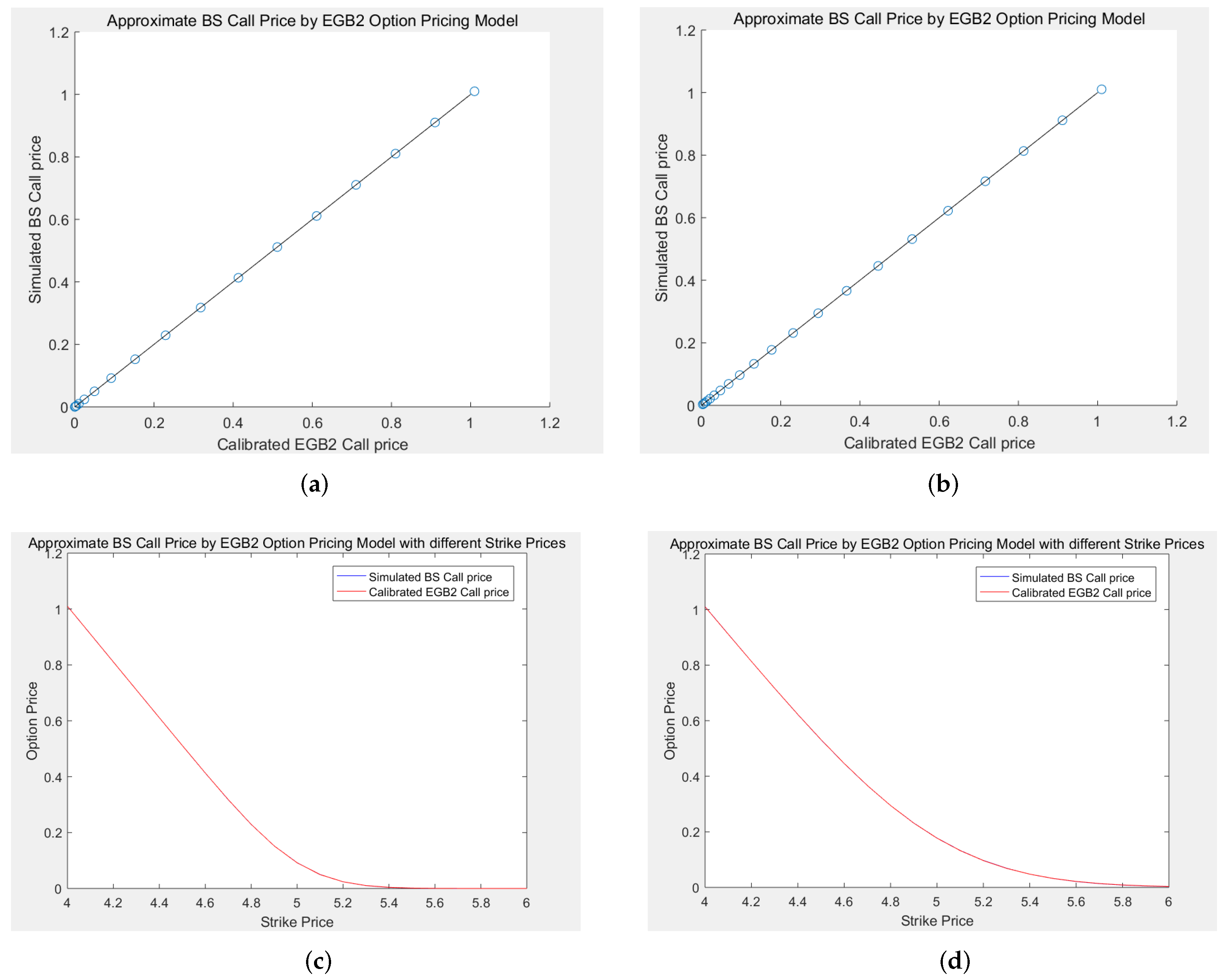
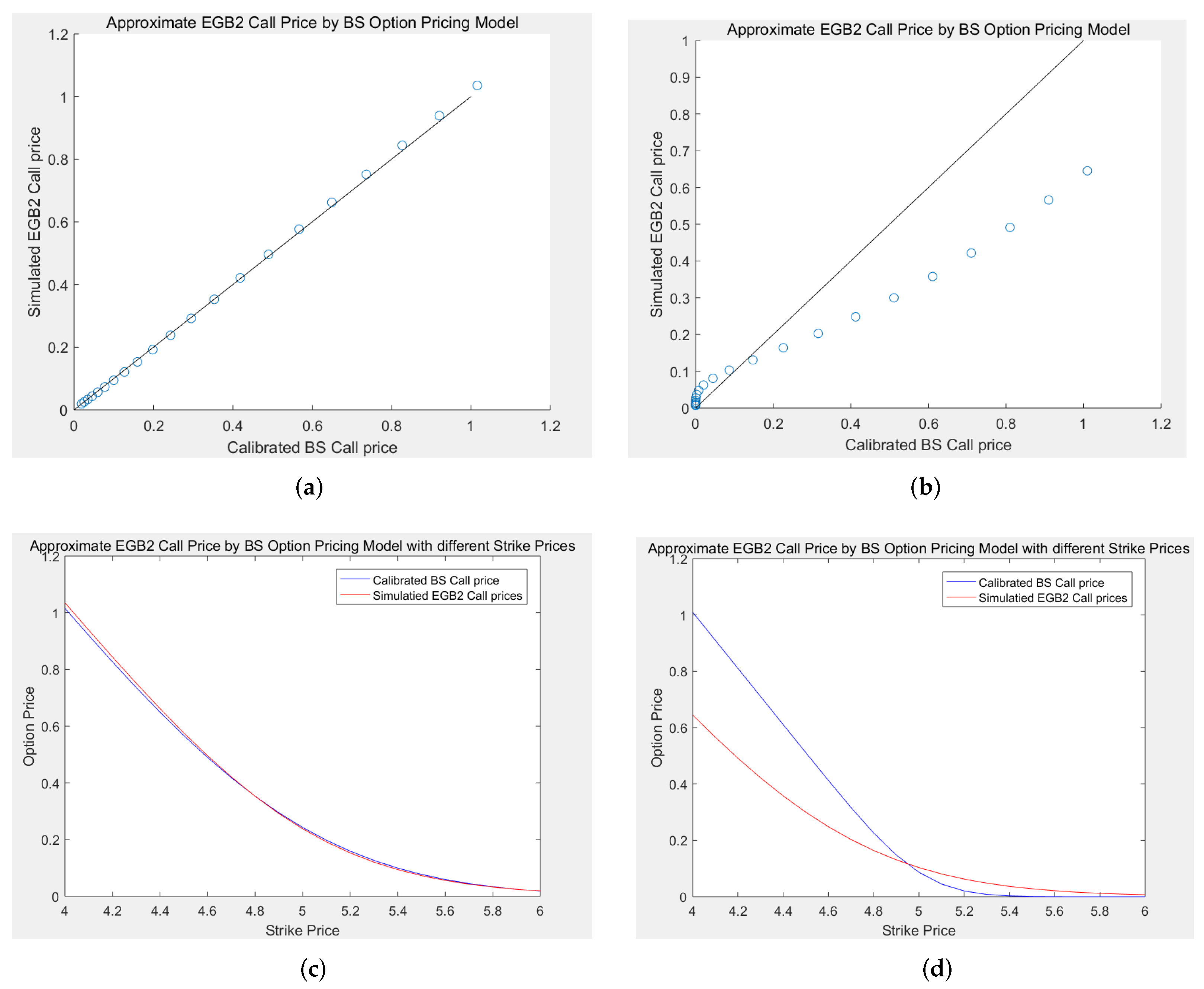
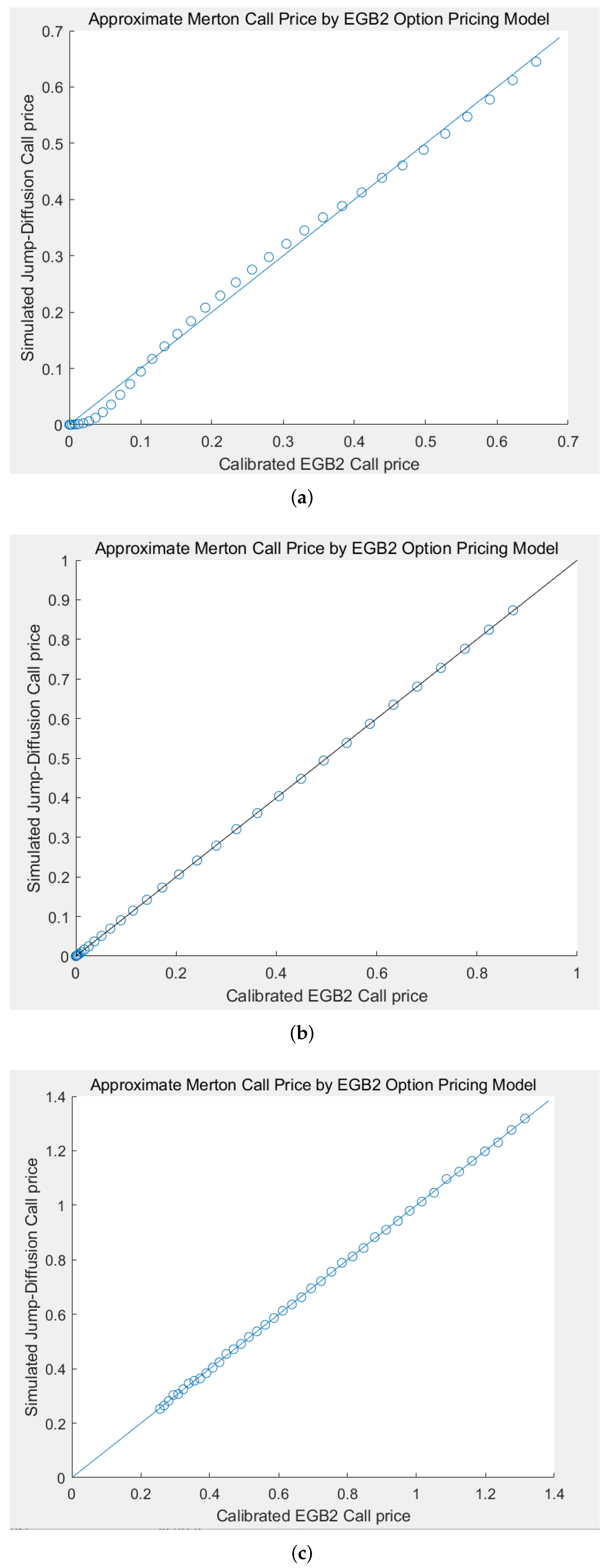
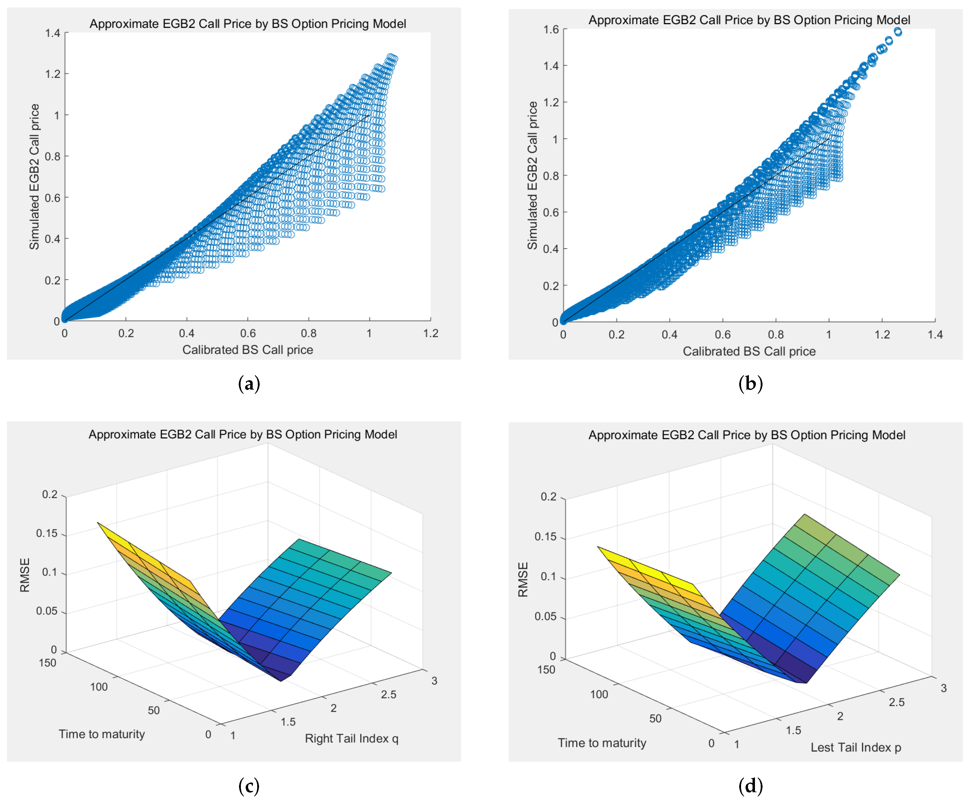
Example 5. 

In this Monte Carlo experiment, each jump-diffusion process is set to have 100,000 paths and 100 nodes. The theoretical prices of Merton’s model are computed by taking the average of the option values over all paths. For comparative purposes, we set $S_t=10$, $r=0.03$, and $T=365$ (days, i.e., 1 year) in each scenario, and examine various moneyness options with strike prices K ranging from 9 to 11 by step size 0.05, i.e., $K=[9,9.05,9.10,\cdots ,10.90,10.95,11]$.

The resulting p-p plots are shown in Figure 4. The RMSEs in three scenarios (financial crisis, market rebound, and normal market) are 0.0127, 0.0007, and 0.0040. The corresponding MAEs are 0.0249, 0.0019, and 0.0260, respectively. Generally speaking, the points in each p-p plot are close to the 45-degree line, and the resulting RMSEs and MAEs are acceptable, meaning that the EGB2OP model has excellent abilities to approximate (or to “replicate”) Merton option prices when K is changing. Among these scenarios, the EGB2OP model provides the best approximation toward Merton’s prices during a market rebound and ideal approximations in a normal market. Admittedly, some of the points in panel (a) of Figure 4 are slightly apart from the 45-degree line. However, this does not mean that the EGB2OP model cannot capture the price change of jump-diffusion models during market turmoils. We can notice that the p-p points in panel (a) of Figure 4 wraps around the 45-degree line and does not contain abrupt change, which means the tiny gaps between the EGB2OP prices and Merton prices are probably computational and negligible.

The real-data pricing performances are compared in

Table 1. Monthly RMSEs and MAEs of the EGB2OP and Merton jump-diffusion (J-D) models over three selected time spans.

Periods	${\mathit{RMSE}}_{\mathit{EGB}2}$	${\mathit{RMSE}}_{\mathit{J}-\mathit{D}}$	${\mathit{MAE}}_{\mathit{EGB}2}$	${\mathit{MAE}}_{\mathit{J}-\mathit{D}}$
Financial Crisis	0.0129	0.9960	0.0246	0.4174
Market Rebound	0.0005	0.5560	0.0056	0.1662
Normal Market	0.0021	0.0040	0.0072	0.1060

. As shown, the EGB2OP model can provide less RMSE and MAE than Merton’s jump-diffusion model in all the scenarios. This means that the jump-diffusion model may not be as practical as the EGB2OP model. In addition, we should note that this comparative analysis is merely in terms of pricing (i.e., the in-sample performance) rather than prediction (i.e., the out-of-sample performance). If predicting ability is considered, the EGB2OP model may outperform all types of jump-diffusion models, as the jump-diffusion setting may entirely model tail risks (i.e., the jumps) stochastically and thus exclude the ability to predict the future. Conversely, the EGB2OP model may detect possible tail risk signals using real data and thus can be used to “report” financial crises. In this regard, this paper proposes three EGB2OP model-based risk reporting tools. See Section 7 for a more detailed tail risk prediction application.

6. Empirical Studies

6.1. Data Description

This section reports the empirical pricing performance of the newly proposed EGB2OP model with reference to the benchmark Black–Scholes model using real data. The data used in this study are the daily closing prices of the SSE 50 ETF (Exchange Traded Funds) call and put options published by the Shanghai Stock Exchange in China. The underlying asset for SSE 50 ETF option is the SSE 50 ETF (trading code: 510050) issued by China Asset Management Co. Ltd. in 2004. To date, the SSE 50 ETF Options are the second-largest option product in the world in terms of trading volume and are very liquid. These options are listed at expiry dates for the near-month, second-near-month, and the following two near-seasons. The expiry date of the SSE 50 ETF option is the fourth Wednesday of the expiration month. The minimum quote unit is 0.0001 Chinese Yuan (RMB). All the options are traded with a contract multiplier of 10,000.

The period of this study is from 16 April 2015 to 28 August 2018. We exclude the observations (1) with zero traded volume on a given day; (2) with time to maturity of less than one week; and (3) violate vertical arbitrage condition. The risk-free rates are the bond markets-based yearly risk-free returns provided by the RESSET database. Except for the risk-free rate, all data used in this study come from the Wind database.

The daily close prices and log-returns of SSE 50 ETF during the sample period are displaced in

Table 2. Descriptive Statistical Analysis of the SSE 50 ETF Daily Close Prices and Daily Log-returns.

Variable, Year	$\mathit{mean}$	$\mathit{max}$	$\mathit{min}$	$0.25\mathit{Quantile}$	$0.75\mathit{Quantile}$
Price, 2015	2.62319	3.42700	1.88600	2.33900	3.00600
Price, 2016	2.19357	2.46000	1.91500	2.11200	2.28125
Price, 2017	2.58310	3.06700	2.29600	2.35675	2.76725
Price, 2018	2.72626	3.18000	2.39000	2.57100	2.88400
Price, Full Sample	2.50453	3.42700	1.88600	2.27900	2.72800
Return, 2015	−0.00065	0.03514	−0.04567	−0.00460	0.00528
Return, 2016	−0.00010	0.01686	−0.02707	−0.00198	0.00202
Return, 2017	0.00040	0.01267	−0.01090	−0.00147	0.00241
Return, 2018	−0.00030	0.01307	-0.02058	−0.00398	0.00299
Return, Full Sample	−0.00011	0.03514	−0.04567	−0.00239	0.00259

. As can be seen from the table, the underlying asset experienced significantly greater extreme losses in terms of mean (−0.00065), minimum (−0.04567), and lower quarter quartile (−0.00460) in the year 2015 than any other year. During the second half of 2015, there was a notable crisis in the Chinese financial investment industry called the “stock disaster” period in the A-share stock market. The descriptive statistical analysis of the underlying assets implies that we need to pay special attention to the out-of-sample risk warning performance of the proposed EGB2OP model during the “stock disaster” period (the second half of 2015) in the empirical analysis. In this regard, we conduct an event study in Section 7.3.

6.2. Methodology

In this paper, we use the probability method to calibrate parameters for the EGB2 option pricing model. For comparison, we also calibrate the B−S model in the same way. The model parameters are estimated by minimizing the sum of squared errors (SSEs) between theoretical prices (of the EGB2OP model or the B−S model) and the real market option prices for each day with the following objective functions:

$$\underset{\theta }{min}SS{E}_{Call}(t,T)=\underset{\theta }{min}\sum _K{[C_t(K,T)-\widehat{C_t}(K,T)]}^2,\forall t,T,$$

(28)

$$\underset{\theta }{min}SS{E}_{Put}(t,T)=\underset{\theta }{min}\sum _K{[P_t(K,T)-\widehat{P_t}(K,T)]}^2,\forall t,T,$$

(29)

where $\theta$ represents the parameter(s) of the objective model. For example, $\theta =(a_{t,T},b_{t,T},p_{t,T},$$q_{t,T})$ for the EGB2OP model, and $\theta =\sigma$ for the B−S model. Using this method, all parameters are risk-neutral parameters and thus can be used to obtain risk-neutral distribution for underlying returns or losses.

Theoretically, if there exists a corresponding future product for an objective option, one can use future prices to simplify the above calibration procedure. To use this method, we need the following martingale condition:

$$F_t=E{{}_t}^Q\left(S_T\right),$$

(30)

where $F_t$ is the future price at time t for the corresponding option (with the same underlying asset and the same time to maturity). Unlike the normal case where the mean of the distribution happens to be the location parameter $\mu$, the mean of the EGB2 distribution is a function of both the location parameter $a_{t,T}$ and the scale parameter $b_{t,T}$, as well as the shape parameters $p_{t,T}$ and $q_{t,T}$. According to McDonald(1991), the mean of an EGB2 distribution can be obtained by its moment-generating function and the first moment in (5).

Based on Equations (5) and (30), using the future prices, the location parameter can be expressed as a function of the forward moneyness and other EGB2 parameters for every given time t:

$$a_{t,T}=ln(S_t/F_t)-b_{t,T}[\phi \left(p_{t,T}\right)-\phi \left(q_{t,T}\right)].$$

(31)

The procedure above is analogous to risk-neutral valuation in the B−S model by replacing $a_{t,T}$ with the risk-free rate of r. Thus, the parameters to be estimated in Equations (28) and (29) become $\theta =(b_{t,T},p_{t,T},q_{t,T})$. One only needs to calibrate three parameters, and therefore, the computational burden can be reduced.

To evaluate the pricing performance of each model, the Root Mean Square Error (RMSE) and Maximum Absolute Error (MAE) are computed. The RMSE is defined as

$$RMSE\left(t\right)=\sqrt{\frac{SSE(t,T)}{N}},$$

(32)

where $SSE(t,T)$ is the SSE for calls or puts calculated by Equations (28) or (29). N represents the number of observations for the given option on a given day. The MAE is defined as

$$MAE\left(t\right)=\sqrt{\frac{{max}_K|C_t(K,T)-\widehat{C_t}(K,T)|}{N}}$$

(33)

for calls, and

$$MAE\left(t\right)=\sqrt{\frac{{max}_K|P_t(K,T)-\widehat{P_t}(K,T)|}{N}}$$

(34)

for puts.

6.3. Empirical Results

6.3.1. Pricing Performance

To demonstrate the pricing performance of the EGB2OP model, we first report the average daily RMSE and MAE for both calls and puts (see

Table 3. Daily Average RMSE and MAE for the EGB2OP and B−S pricing models.

Type, Year	${\mathit{RMSE}}_{\mathit{EGB}2}$	${\mathit{RMSE}}_{\mathit{B}-\mathit{S}}$	${\mathit{MAE}}_{\mathit{EGB}2}$	${\mathit{MAE}}_{\mathit{B}-\mathit{S}}$
Call, 2015	0.01231	0.02619	0.02427	0.03334
Call, 2016	0.00075	0.02499	0.00717	0.03614
Call, 2017	0.00070	0.03001	0.00704	0.03015
Call, 2018	0.00150	0.02026	0.00839	0.01785
Call, Full Sample	0.00576	0.02680	0.01320	0.03020
Put, 2015	0.01871	0.02206	0.02862	0.03079
Put, 2016	0.00053	0.01072	0.00585	0.02057
Put, 2017	0.00051	0.01276	0.00578	0.01677
Put, 2018	0.00398	0.01131	0.01269	0.02026
Put, Full Sample	0.00511	0.01387	0.01211	0.02623

) Then, as a reference and comparison, the pricing results of the B−S formulas are also reported.

As is shown in Table 3, the EGB2OP model yields smaller RMSE and MAE than the corresponding B−S results for both calls and puts in each year as well as overall. The dynamics of RMSE and MAE for both models are displayed in Figure 5a and Figure 5b, respectively. For these results, one can find: (1), the EGB2OP model outperforms the B−S model in terms of RMSE and MAE almost all the time; (2), in 2015, there is not much difference between the RMSEs and MAEs of the EGB2OP and the B−S pricing models for both calls and puts, although the EGB2OP still provides smaller RMSE and MAE than the B−S. However, after 2015, the RMSEs and MAEs of the EGB2OP are significantly smaller than those of the B−S. One reason for this could be the structural and financial policy change in China’s stock market in early January 2016, after the “stock disaster” period in 2015.

6.3.2. Implied Moments

In this subsection, we report the dynamics of the EGB2OP model implied moments for both calls and puts. For the second moment, the dynamics of the B−S implied volatilities are shown as a reference and comparison, while for higher moments, only the results of the EGB2OP model are reported.

The EGB2OP implied standard deviation and the B−S implied volatility for the next-month, the near-season, and the next-season are shown in Figure 6a, Figure 6b, and Figure 6c, respectively. The standard deviations of the EGB2OP are computed by computing the square root of the Equation (6). As shown, the EGB2OP standard deviations share the same term structure with the B−S implied volatilities. In turmoil time (2015 and 2018), the EGB2OP standard deviations are very close to the corresponding B−S implied volatilities. But in stable markets (2016 and 2017), the EGB2 standard deviations are relatively lower than the corresponding B−S implied volatilities. Such results mean that the EGB2OP model provides a consistent measure for the second moments of underlying returns/losses of the B−S in the bull markets or bear markets but provides a smaller value than the B−S in stable markets. However, one point of view we shall highlight here is that the EGB2OP model provides significantly lower RMSEs and MAEs than the B−S model in the periods when markets are stable, indicating that the B−S implied volatility could be too conservative in stable periods.

Higher-order moments such as implied skewness and kurtosis (see Equations (9) and (10)) for the next-month, the near-season, and the next-season, are exhibited in Figure 7. In the sample period, the skewnesses range from $\pm 2$ and usually lie between $\pm 1.5$, significantly different from zero. The kurtoses range from 3 to 9, usually between 4 to 7, larger than 3, which happens to be the kurtosis of normal distribution. The empirical results for the third and fourth moments indicate that the underlying returns/losses may not follow the normality since the EGB2OP implied skewness and kurtosis always depart from 0 and 3, respectively.

7. Model-Based Instruments for Tail Risk Signals Detection

Asset pricing and risk analysis are two sides of a coin. Serving as one of the novelties of this paper, this section proposes three model-based instruments to detect tail risk signals from option prices. The first instrument is the tail risk index, which can directly measure tail risk constructed using EGB2 parameters. The second instrument is the EGB2 implied Value at Risk (EGB2-VaR), which quantifies the extent of possible financial losses underlying the EGB2 setting. Via daily calibration of the pricing models, dynamic tail risk signals curves can be obtained using these two instruments. In Section 7.1 and Section 7.2, we demonstrate their powerful tail risk detection and early warning abilities by using real data. The third tool is the EGB2 implied risk-neutral density, which detects tail risk signals in a static way. In Section 7.3, we conduct an event study using the data during the 2015 “stock disaster” in China’s market and demonstrate that the EGB2 implied R.N.D. do provide timely beforehand warnings showing asymmetry in underlying’s losses.

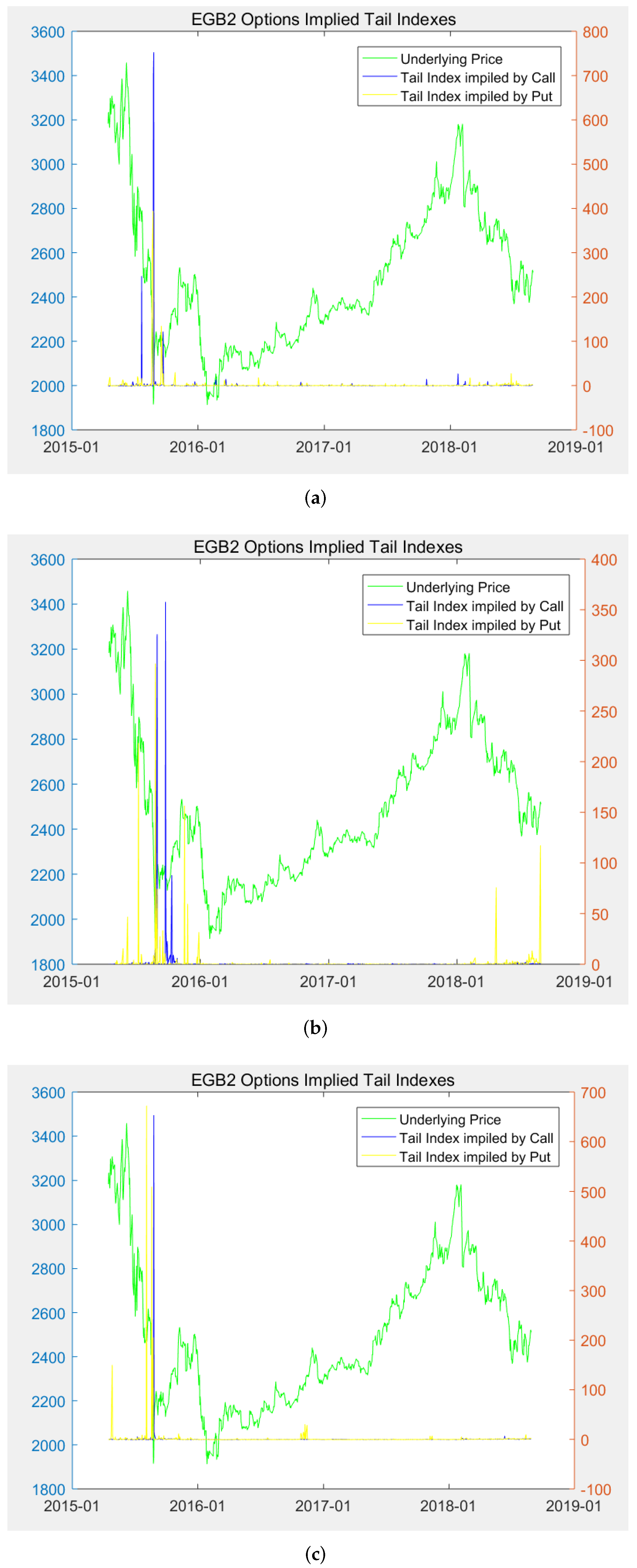
7.1. The EGB2 Implied Tail Risk Index

The tail risk index proposed in this subsection is analogous to the B−S volatility but reflects returns’ asymmetry and market views towards tail risks (the newly proposed measure is termed “implied tail risk index”, or for short, “tail index”). The tail index is constructed using EGB2OP model parameters. Thus, once the model is calibrated, the implied tail (risk) index can be obtained.

The EGB2OP implied tail index $\eta$ (or ${\eta }_{t,T}^c$ for call options and ${\eta }_{t,T}^p$ for put options) defined as:

$${\eta }_{t,T}^c=\frac{p_{t,T}^c-q_{t,T}^c}{q_{t,T}^c}$$

(35)

and

$${\eta }_{t,T}^p=\frac{p_{t,T}^p-q_{t,T}^p}{q_{t,T}^p}$$

(36)

where $p_{t,T}^c$ and $q_{t,T}^c$ are the implied left tail parameter and the implied right tail parameter based on the calibration results of time t with maturity date T. One can obtain the EGB2OP implied tail indexes dynamics for both calls and puts by calibrating each day’s EGB2 option pricing model. Ideally, the EGB2 implied tail indexes ${\eta }_{t,T}^c$ and ${\eta }_{t,T}^p$ should be able to reflect the investors’ opinions about tail risks by trading options. If the tail index is positive, i.e., the implied left tail parameter $p_{t,T}$ is larger than the implied right tail parameter $q_{t,T}$ for losses, the underlying R.N.D. for losses in the future is skewed to the right, and the tail probability for big loss is much larger than big gain. When ${\eta }_{t,T}$ is positive and extremely large, it is a warning for a bear market or financial crisis. If the tail index is negative, the implied left tail parameter $p_{t,T}$ is smaller than the implied right tail parameter $q_{t,T}$, i.e., the underlying R.N.D. for losses is skewed to the left, and the tail probability for big gain is larger than a big loss. When ${\eta }_{t,T}$ is negative and close to $-1$, it is an indicator of a bull market, and investors are optimistic about the future in terms of “small probability to win a big deal”. The construction of the tail index and the interpretation of the parameters p and q also demonstrate the financial interpretability of the EGB2OP model.

Figure 8 exhibits dynamics of the model-based EGB2 implied tail indexes for the next-month, the near-season, and the next-season. For illustrative purposes, we display the underlying price dynamic in each panel as well. As can be seen from the figures, the tail index ${\eta }_{t,T}$ is not far away from 0 except for the time when the markets are at risk. For example, there is a period when implied tail indexes are very large from August 2015 to October 2015, which happens to be a “stock disaster” period in China. The tail indexes were over 3200 for both calls and puts at that time, indicating a financial crisis. Such a warning was meaningful for tail risk management at that time. For studying the use of the EGB2 implied tail indexes and the implied R.N.D. for tail risk warning, we undertake an event study in the next subsection.

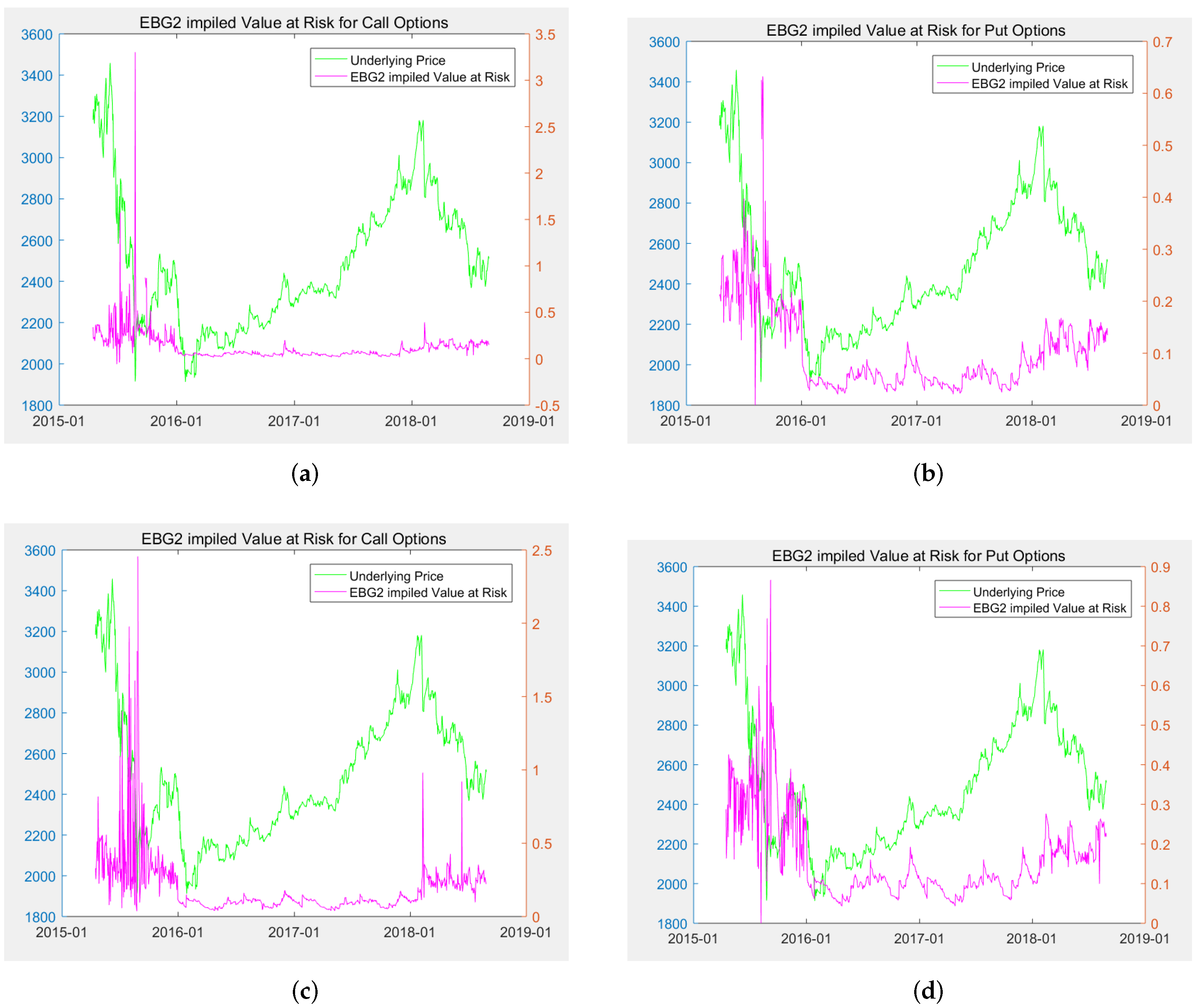
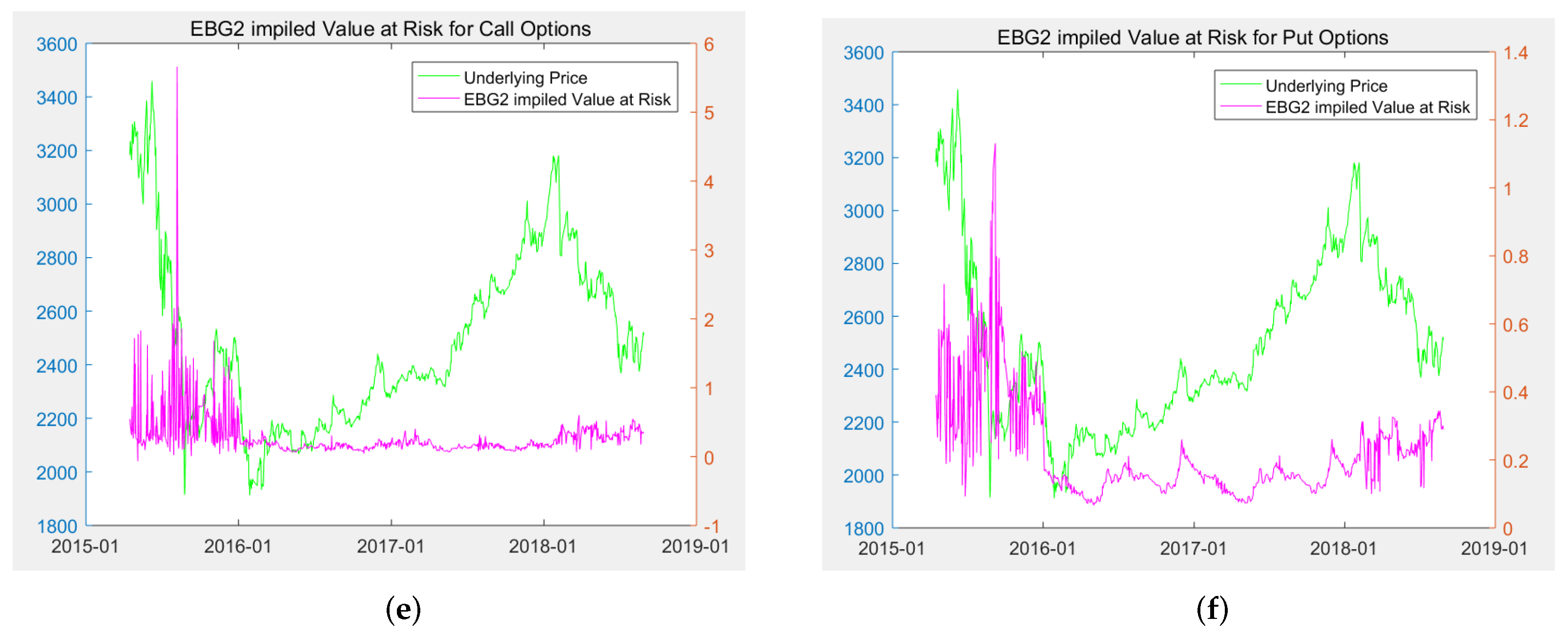
7.2. The EGB2 Implied Value at Risk

The second model-based risk measuring instrument is the EGB2 implied Value at Risk (EGB2-VaR). Compared to the method for computing conventional Value at Risk (VaR), the EGB2-VaR is defined as the upper $\alpha$ quantile of R.N.D. of the underlying losses:

$$Va{R}_{\alpha }^{EGB2}\left(X\right)=sup\{x\in \mathbb{R}:F_X\left(x\right)<1-\alpha \}$$

(37)

where $F_X$ is the Cumulative Distribution Function (C.D.F.) of R.N.D Equation (13) using calibrated parameters. Theoretically, a higher value of EGB2-VaR means a stronger signal for tail risk warning.

The implied EGB2-VaR dynamics when $\alpha =0.05$ are shown in Figure 9. As shown, both the implied EGB2-VaR for calls and puts reach substantial values from August 2015 to October 2015, which can be seen as signals of tail risk warning. Similarly, the implied EGB2-VaR for the near-season and the next-month calls also puts signal crisis warnings in January 2018 and April 2018. Those results are evidence that EGB2-VaR can be a powerful tool for tail risk signals detection.

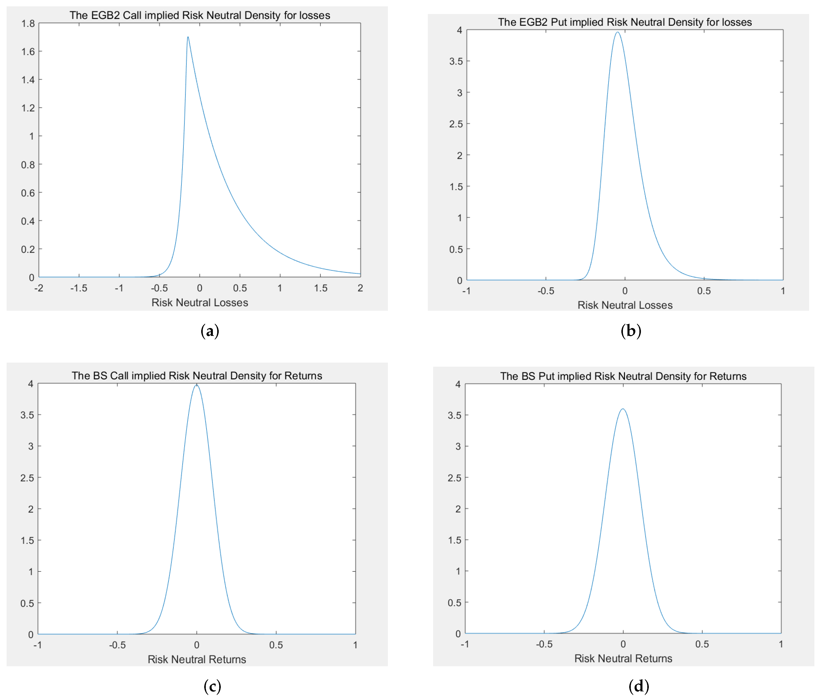
7.3. Event Study and the EGB2 Implied Risk-Neutral Density

In practice, the essential element for an option pricing model to reflect the market view and predict the future is the risk-neutral density (R.N.D.). If a model does provide a good mirror of the market’s view, the ex-ante predicting performance is crucial. This paper assumes that it is the negative logarithmic losses rather than the underlying prices that follow the EGB2 distribution. This assumption, in turn, yields the EGB2 model-based R.N.D. for losses, which has great flexibility for capturing tail behavior and fat tail phenomena of markets. In this subsection, we undertake an event study for a bear market time and use one-day-ex-ante R.N.D. The B−S R.N.D.s are also provided in this study as a reference and comparison.

The maximum daily losses for the underlying asset (SSE 50 ETF, trading code: 510050) over our sample period is on the date of 24 August 2015. To examine the one-day-ex-ante prediction performance, we display the EGB2OP implied R.N.D. for loss, and the B−S implied R.N.D. for profit/loss in the last trading date, 21 August 2015. For illustrative reasons, we choose the next-month as an example because it provides the best sensitivity.

The R.N.D. for losses implied by the EGB2OP calls and puts are shown in Figure 10a and Figure 10b, respectively. As a comparison, the R.N.D. for returns implied by the B−S model are shown in Figure 10c,d for calls and puts. As shown in Figure 10a,b, one day before the extreme crisis came for both calls and puts, the EGB2OP implied R.N.D. of losses were already exhibiting significantly positive skewness and fat tails on the right, which implies that large losses are possible, but high returns are almost impossible. Such results could be an effective warning of the negative sentiment in the market about the ongoing crisis. However, according to Figure 10c,d, the B−S implied R.N.D. for returns are symmetric for both calls and puts without exhibiting any fat-tail features. Based on the B−S pricing results, one can hardly infer or obtain the market view about the upcoming crisis. Those results evidence that the EGB2 R.N.D. is an ideal static measure for detecting tail risk signals.

8. Conclusions, Implications, and Future Research Directions

8.1. Conclusions and Implications

This paper proposes a novel option pricing model based on the EGB2 distribution, which includes the B−S formula as a limit case and can perfectly “replicate” Merton’s option prices. The generality and interpretability guarantee that the proposed model can capture price behaviors in both peace market periods and financial crises. The pricing accuracy is shown by an empirical study using China’s options data.

We note that the reason why the proposed model has the above ideal properties is because of the powerful structure of the EGB2 distribution per se, rather than the utilization of many parameters. First of all, the EGB2 distribution includes normal and many other distributions as limit cases, which makes it possible for the EGB2OP model to perfectly “replicate” the B−S and Merton’s prices, demonstrating its generality. In addition, due to the flexibility provided by the two tail parameters, the pricing model can guarantee its pricing abilities in both asymmetrical (crises) and symmetrical (normal) cases, which indicates its robustness.

Based on our option pricing model, three tail risk measures (EGB2 tail risk index, EGB2-VaR, and EGB2 R.N.D.) are proposed, all of which are shown to be powerful indicators of tail risks. In practice, investors and policymakers can detect potential tail risk signals by tracing the dynamics of the EGB2-tail risk index and EGB2-VaR. Extremely large values in EGB2 tail indexes and EGB2-VaR are timely warning signals for upcoming crises.

In practice, the proposed EGB2OP model and three model-based tail risk signals detecting tools may offer important implications for policymakers, portfolio managers, and derivatives traders. From a macro level, policymakers can effectively understand the ”market view” of tail risks from the option market to take the lead in using preventive policies before the financial crisis (such as providing timely capital liquidity and market liquidity to the market) macro-level tail risk hedging. At the micro level, portfolio managers can fully use the three tail risk detection tools for portfolio optimization to avoid huge losses (liquidation risks) in a rapidly changing market situation. Meanwhile, since the proposed option pricing model results in better pricing accuracy, it would also be beneficial for asset management companies to conduct more accurate asset pricing when trading derivatives and issuing OTC derivatives.

8.2. Further Study Directions

The proposed EGB2OP model and three model-based tail risk signals detecting instruments might offer a novel benchmark for detecting tail risk signals from option prices, based on which many further studies can be conducted in the future.

First, extending the proposed EGB2OP model into a more general form would be of academic significance. The proposed model is a static model with only a single asset. To make it more general, one can modify the EGB2OP model into a dynamic version by modeling four model parameters with time-series approaches or extend the model into a multi-assets case using multivariate statistical methods.

Second, from an applied perspective, it would be of practical significance to link the EGB2OP model with risk hedging. In this regard, novel EGB2OP model-based Greeks and corresponding tail risk hedging strategies can be further investigated.

Last but not least, this study might offer more hints and implications for complicated option pricing research. In this paper, the proposed model targets the vanilla option, which is the simplest type of option. But it would be necessary to consider tail risk effects and leptokurtic features of asset returns when dealing with more complicated option pricing issues. In the future, EGB2OP model-based pricing algorithms can be further proposed for pricing exotic products such as barrier options, backdating options, and Asian options.

References

1. Safdar, I.; Neel, M.; Odusami, B. Accounting information and left-tail risk. Rev. Quant. Financ. Account. 2022, 58, 1709–1740. [Google Scholar] [CrossRef]
2. Brown, J.; Çakır Melek, N.; Matschke, J.; Sattiraju, S.A. The Missing Tail Risk in Option Prices. In Federal Reserve Bank of Kansas City Working Paper 23-02; Federal Reserve Bank of Kansas City: Kansas City, MO, USA, 2023. [Google Scholar] [CrossRef]
3. Kou, S.G. A jump-diffusion model for option pricing. Manag. Sci. 2002, 48, 1086–1101. [Google Scholar] [CrossRef] [Green Version]
4. Kou, S.G.; Wang, H. Option pricing under a double exponential jump diffusion model. Manag. Sci. 2004, 50, 1178–1192. [Google Scholar] [CrossRef] [Green Version]
5. McDonald, J.B.; Michelfelder, R.A. Partially adaptive and robust estimation of asset models: Accommodating skewness and kurtosis in returns. J. Math. Financ. 2016, 7, 219–237. [Google Scholar] [CrossRef] [Green Version]
6. Bhansali, V. Tail risk management. J. Portf. Manag. 2008, 34, 68–75. [Google Scholar] [CrossRef]
7. Bhansali, V. Tail Risk Hedging: Creating Robust Portfolios for Volatile Markets; McGraw-Hill Education: New York, NY, USA, 2014. [Google Scholar]
8. Bhansali, V.; Davis, J.M. Offensive risk management II: The case for active tail hedging. J. Portf. Manag. 2010, 37, 78–91. [Google Scholar] [CrossRef]
9. Bhansali, V.; Chang, L.; Holdom, J.; Rappaport, M. Monetization Matters: Active Tail Risk Management and the Great Virus Crisis. J. Portf. Manag. 2020, 47, 16–28. [Google Scholar] [CrossRef]
10. Bhansali, V. Behavioral Perspectives on Tail-Risk Hedging. J. Invest. 2015, 24, 122–133. [Google Scholar] [CrossRef]
11. Harlow, R.L.; Hubrich, S.; Page, S. Tail Risk Hedging in a Low-Rate Environment. J. Deriv. 2022, 29, 110–120. [Google Scholar] [CrossRef]
12. Chang, L.; Holdom, J.; Bhansali, V. Tail Risk Hedging Performance: Measuring What Counts. J. Portf. Manag. 2022, 48, 25–39. [Google Scholar] [CrossRef]
13. Lin, H.; Liu, L.; Zhang, Z. Hedging and Evaluating Tail Risks via Two Novel Options Based on Type II Extreme Value Distribution. Symmetry 2021, 13, 1630. [Google Scholar] [CrossRef]
14. McDonald, J.B.; Bookstaber, R.M. Option pricing for generalized distributions. Commun. Stat.-Theory Methods 1991, 20, 4053–4068. [Google Scholar] [CrossRef]
15. Fischer, M.J. The Esscher-EGB2 Option Pricing Model; No. 31/2000; Diskussionspapiere//Friedrich-Alexander-Universität Erlangen-Nürnberg, Lehrstuhl für Statistik und Ökonometrie: Nürnberg, Germany, 2000. [Google Scholar]
16. Mirfendereski, D.; Rebonato, R. Closed-form solutions for option pricing in the presence of volatility smiles: A density-function approach. J. Risk 2001, 3, 5–26. [Google Scholar] [CrossRef]
17. Markose, S.M.; Alentorn, A. The generalized extreme value distribution, implied tail index, and option pricing. J. Deriv. 2011, 18, 35–60. [Google Scholar] [CrossRef] [Green Version]
18. Kim, J.; Kim, H.-O. Option Implied Tail Index and Volatility Based on Heavy-tailed Distributions: Evidence from KOSPI 200 Index Options Market. Glob. Econ. Rev. 2014, 43, 269–284. [Google Scholar] [CrossRef]
19. De Jong, C.; Huisman, R. From skews to a skewed-t: Modelling option-implied returns by a skewed student-t. In Proceedings of the IEEE/IAFE/INFORMS 2000 Conference on Computational Intelligence for Financial Engineering (CIFEr) (Cat. No. 00TH8520), New York, NY, USA, 28 March 2000; IEEE: Piscataway, NJ, USA, 2000; pp. 132–142. [Google Scholar]
20. Madan, D.B.; Carr, P.P.; Chang, E.C. The variance gamma process and option pricing. Rev. Financ. 1998, 2, 79–105. [Google Scholar] [CrossRef] [Green Version]
21. Savickas, R. A simple option pricing formula. Financ. Rev. 2002, 37, 207–226. [Google Scholar] [CrossRef]
22. Chen, Y.; Cai, Y.; Zheng, C. Estimation of Tail Risk and Moments Using Option Prices with a Novel Pricing Model under a Distorted Lognormal Distribution. Math. Probl. Eng. 2020, 2020, 1603509. [Google Scholar] [CrossRef]
23. Aboura, S.; Valeyre, S.; Wagner, N. Option pricing with a dynamic fat-tailed model. J. Deriv. Hedge Funds 2014, 20, 131–155. [Google Scholar] [CrossRef]
24. Fisher, R.A.; Tippett, L.H.C. Limiting forms of the frequency distribution of the largest or smallest member of a sample. In Mathematical Proceedings of the Cambridge Philosophical Society; Cambridge University Press: Cambridge, UK, 1928; Volume 24, pp. 180–190. [Google Scholar]
25. Cox, J.C.; Ross, S.A. The valuation of options for alternative stochastic processes. J. Financ. Econ. 1976, 3, 145–166. [Google Scholar] [CrossRef]
26. Black, F.; Scholes, M. The pricing of options and corporate liabilities. J. Political Econ. 1973, 81, 637–654. [Google Scholar] [CrossRef] [Green Version]
27. McDonald, J.B.; Xu, Y.J. A generalization of the beta distribution with applications. J. Econom. 1995, 66, 133–152. [Google Scholar] [CrossRef]
28. McDonald, J.B. Parametric models for partially adaptive estimation with skewed and leptokurtic residuals. Econ. Lett. 1991, 37, 273–278. [Google Scholar] [CrossRef]
29. Lin, H.; Zhang, Z. Extreme co-movements between infectious disease events and crude oil futures prices: From extreme value analysis perspective. Energy Econ. 2022, 110, 106054. [Google Scholar] [CrossRef]
30. Kerman, S.C.; McDonald, J.B. Skewness-Kurtosis Bounds for EGB1, EGB2, and Special Cases. Commun. Stat.-Theory Methods 2015, 44, 3857–3864. [Google Scholar] [CrossRef]
31. Yang, X.; Frees, E.W.; Zhang, Z. A generalized beta copula with applications in modeling multivariate long-tailed data. Insur. Math. Econ. 2011, 49, 265–284. [Google Scholar] [CrossRef]
32. Harris, R.D.F.; Küçüközmen, C.C. The empirical distribution of UK and US stock returns. J. Bus. Financ. Account. 2001, 28, 715–740. [Google Scholar] [CrossRef]
33. Wang, Y.-M.; Li, C.-A.; Lin, C.-F. The impact of investor sentiment on the futures market: Evidence from the Taiwan futures exchange. Int. Res. J. Financ. Econ. 2009, 28, 134–151. [Google Scholar]
34. Ayala, A.; Blazsek, S. Score-driven models of stochastic seasonality in location and scale: An application case study of the Indian rupee to USD exchange rate. Appl. Econ. 2019, 51, 4083–4103. [Google Scholar] [CrossRef]
35. Ayala, A.; Blazsek, S.; Licht, A. Score-driven stochastic seasonality of the Russian rouble: An application case study for the period of 1999 to 2020. Empir. Econ. 2022, 62, 2179–2203. [Google Scholar] [CrossRef]
36. Ji, J.; Lin, H. Evaluating Regional Carbon Inequality and Its Dependence with Carbon Efficiency: Implications for Carbon Neutrality. Energies 2022, 15, 7022. [Google Scholar] [CrossRef]
37. Harrison, J.M.; Pliska, S.R. Martingales and stochastic integrals in the theory of continuous trading. Stoch. Process. Their Appl. 1981, 11, 215–260. [Google Scholar] [CrossRef] [Green Version]
Figure 1. Comparisons of C t ( δ ) ( K ) with different δ and C t B S ( K ) on three options’ moneyness types ATM, ITM, and OTM with varying b values on the horizontal axis. The blue curves are the theoretical B−S prices and the green intervals are the sets of all possible EGB2OP prices, accordingly. As can be seen from the figure, the B−S price lines are almost always right in the middle of the EGB2 prices belt in each case, which gives a sense that the EGB2OP price indeed goes to a limit of the B−S price. (a) Comparisons of C t ( δ ) ( K ) with different δ and C t B S ( K ) for ATM Options; (b) Comparisons of C t ( δ ) ( K ) with different δ and C t B S ( K ) for ITM Options; (c) Comparisons of C t ( δ ) ( K ) with different δ and C t B S ( K ) for OTM Options.
Mathematics 11 03194 g001aMathematics 11 03194 g001b
Figure 2. Resulting plots for Examples 1 and 2. (a) Price to Price plot with the B−S model using σ = 0.15 ; (b) Price to Price plot with the B−S model using σ = 0.3 ; (c) Option prices with different strike prices with the B−S model using σ = 0.15 ; (d) Option prices with different strike prices with the B−S model using σ = 0.30 .
Mathematics 11 03194 g002
Figure 3. Resulting plots for Example 3 and Example 4. (a) Price to Price plot with EGB2 q t , T = 2 ; (b) Price to Price plot with the EGB2OP using q t , T = 1 ; (c) Option prices with different strike prices when the EGB2OP using q t , T = 2 ; (d) Option prices with different strike prices with the EGB2OP using q t , T = 1 .
Mathematics 11 03194 g003
Figure 4. Comparisons of the simulated option prices from Merton’s Jump-Diffusion Model and the calibrated EGB2OP model prices in varieties of market environments: (a) financial crises; (b) rebound; and (c) normal market.
Mathematics 11 03194 g004
Figure 5. Empirical Results: (a) The RMSEs dynamics for the EGB2OP and B−S models; (b) The MAEs dynamics for the EGB2OP and B−S models.
Mathematics 11 03194 g005
Figure 6. The EGB2 implied standard deviation and B−S implied volatility for the contracts of the: (a) next-month; (b) near-season; (c) next-season.
Mathematics 11 03194 g006
Figure 7. Implied results for the third and fourth moments: (a) The EGB2 implied skewness for the next-month; (b) The EGB2 implied kurtosis for the next-month; (c) The EGB2 implied skewness for the near-season; (d) The EGB2 implied kurtosis for the near-season; (e) The EGB2 implied skewness for the next-season; (f) The EGB2 implied kurtosis for the next-season.
Mathematics 11 03194 g007
Figure 8. The EGB2 implied tail indexes for: (a) the next-month; (b) the near-season; (c) the next-season.
Mathematics 11 03194 g008
Figure 9. The EGB2 implied VaR for the: (a) next-month calls; (b) next-month puts; (c) near-season calls; (d) near-season puts; (e) next-season calls; (f) next-season puts.
Mathematics 11 03194 g009aMathematics 11 03194 g009b
Figure 10. Implied R.N.D. for losses one day before crisis: (a) EGB2 Call; (b) EGB2 Put; (c) B−S Call; (d) B−S Put.
Mathematics 11 03194 g010