Abstract
In this paper, we use a similar approach to the one proposed by Chen and Jiao to calculate the mathematical formulas of the generating function and the mass function of a cross-talking pathways model in large parameter regions. Together with kinetic rates from yeast and mouse genes, our numerical examples reveal novel bimodal mRNA distributions for intermediate times, whereby the mode of distribution displays unimodality with the peak at for initial and long times, which has not been obtained in previous works. Such regulation of mRNA distribution exactly matches the transcriptional dynamics for the osmosensitive genes in Saccharomyces cerevisiae, which has not been generated by those models with one single pathway or feedback loops. This paper may provide us with a novel observation on transcriptional distribution dynamics regulated by multiple signaling pathways in response to environmental changes and genetic perturbations.
Keywords:
stochastic gene transcription; cross-talking pathways; probability mass function; intermediate dynamical bimodal distribution MSC:
34K05; 92C37; 92C40
1. Introduction
Gene transcription is a central and stochastic process in cells, through which, the genetic information stored in DNA is transcribed into mRNA molecules, which are then translated into proteins. The stochasticity and bursting fashion of transcription were widely studied both in experiments and theoretical research in the last two decades [1,2,3,4]. The stochasticity is manifested by the heterogeneous distribution of mRNA copy numbers in the population of isogenic cells [4,5,6,7]. The probability mass function , which is the probability that there are exactly m mRNA copies of the gene at time t in one cell, is often used to quantify fluctuations in mRNA levels. By using recent single-cell measurements [8,9] and parameter estimation methods [10,11,12,13], we can obtain massive data on the histogram of the probability mass function [9,14,15]. The distribution profiles of have been studied in [16,17,18,19,20]. They found that there are three types of distribution: decaying distribution, for which, decreases in m; unimodal distribution, for which, peaks uniquely at ; biomodal distribution, for which, has two peaks: one is at and the other is at some .
The two-state model is considered as one of the most classic models to understand how varying external signals influence the profile of . As shown in the diagram
the gene is suggested to switch randomly between off (inactive) and on (active) states [2,4], where is the activation rate and is the inactivation rate. The processes of the birth and death of mRNAs are determined by the synthesis rate and the degradation rate , respectively. Some indices of this model, such as the mean, noise, fano factor and probability distribution , have been applied to fit the experimental data obtained in yeast [21], bacteria [22] and mammals [23]. However, some inducible genes in the important physiological processes, such as immunity, development and stem cell renewal, are activated by multiple pathways [24,25,26]. Modeling the transcription by a single signal pathway cannot be sufficient in capturing the multiple biochemical reactions. Therefore, some authors introduced transcription models with two or more competitive cross-talking pathways responding to environmental changes [6,27,28,29,30,31]. The cross-talking model can be generalized as the following diagram,
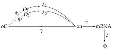
The two competitive cross-talking pathways can activate the transcription alternatively. Here, we use to denote the induction strength of the first pathway and to denote the induction strength of the second one, where
Let denote the gene off state if the gene is transferred to the gene on state by the ith pathway. The pathway selection probabilities are denoted by
and satisfy
Other parameters , v and are in accordance with the two-state model (1). Then, the gene switches randomly between off (inactive) and on (active) states, and the respective probabilities of m mRNA molecules existing at time t with the j-th pathway being chosen are defined as . We let denote the probability that there are m mRNA molecules and the gene resides at an active state. Then, the total probability mass function is
According to the standard procedure in the theory of stochastic processes [31], the three partial mass functions satisfy the following system of master equations
where . Without a loss of generality, we assume that the gene is inactive and the number of transcripts is zero at . Then, the initial condition is
We define the probability generating functions [19,32] as
Then, the initial value problem of the master Equations (3)–(5) is transformed into a system of first-order partial differential equations
with the initial condition
By adding the three solutions of the initial value problem (8)–(11) together and then applying the conversion formula, we obtain as
where and . We introduce non-dimensionalized system parameters
and two real numbers determined by algebra equation
Recently, Zhu, Han and Jiao [20] studied the dynamical regulation of mRNA distribution produced in a transcription system activated by two competitive cross-talking pathways. They expressed distribution in mathematical dynamical formula under the moderate regulation, and displayed the dynamical transitions from mRNA decaying distribution to unimodal distribution undergoing the significant intermediate bimodal stage for stress genes in yeast. In this work, we continue to study the transcription model activated by two competitive cross-talking pathways via introducing a similar approach to the one in [16] to derive the mathematical formulas of the generating function and mass function . Meanwhile, we get a dynamical bimodal distribution that is different from the results in [20].
The rest of this paper is organized as follows. In Section 2 and Section 3, we express mathematical formulas of the generating function and the distribution , respectively. We then give some numerical simulations to illustrate the dynamical bimodal distribution in Section 4. Finally, conclusions and discussion are given in Section 5.
2. Expressing Generating Function
In this section, we use a novel approach to calculate the analytical formula of the generating function in a special parameter region.
Theorem 1.
If , and , the generating function can be expressed as
where
Proof.
For , and , without a loss of generality, we suppose and . Moreover, we let be the generalized hypergeometric function [33], which is denoted by
Thus, is equal to 1 if it contains or
Let be a parameter and
Then, we transform Equations (8)–(10) into ordinary differential equations [20,34],
By introducing a further transformation
we obtain . Then, Equations (17)–(19) can be transformed into
We give a linear operator as
and then prove that is the unique solution of the following initial value problem
by using a similar calculation to the one in [6], where a, b, c and d are real constants and is a smooth function of x.
Since in (25) is the generalized hypergeometric equation, then, if , there are three independent particular solutions of , that is,
Then, the general solution for is derived and given as
where A, B and C are undetermined constants. By substituting the inial value condition and into (29), we can obtain the following system of equations:
where
In order to solve Equations (30)–(32), multiplying (32) by and adding (30) lead to
Using the same method, we multiply (32) by and add (31), then obtain
By a straightforward calculation, we solve (33) and (34) and obtain
where is the of , and , namely,
We substitute (35) and (36) into (32) and obtain
Differentiating the generalized hypergeometric function, we obtain
and
Applying (26)–(28), (39) and (40) leads to
We set
Then, we verify (47). Due to the fact that , and are three independent solutions of the third order ordinary differential equation , for any given real number , has the following form:
Since is arbitrary, we could let . Moreover, we have by calculation. Substituting (26)–(28), (37) and (41)–(46) into (48), we obtain (47) immediately.
Noting that [16]
and
We can further simplify and as
where is the confluent hypergeometric function, which is the following:
We now denote as a gamma function, and rewrite the Euler’s integral for and as follows [35]:
when and , where
Moreover, we note that . Together with (58) and (59), it is easy to calculate that
We can obtain the integral expression of immediately by substituting (60)–(64) into (69). The proof of Theorem 1 is completed. □
3. Expressing Mathematical Formulas of the Distribution
In this section, we express mathematical formulas of the distribution in the same parameter region that was given in the last section.
Theorem 2.
If , and , the probability mass function can be expressed as
and when ,
4. Dynamical Bimodal Distribution
In this section, we will demonstrate through numerical examples that competitive cross-talking pathways can generate new dynamics within several parameter regions compared with [20].
In growing yeast cells, transcripts are turned over rapidly, with a median mRNA half-life of min [36], so the degradation rate min. The upper bound of total transcripts gives the transcription rate, which is min. From the burst size , we obtain min. The selection probabilities of the two pathways are given as and . Set a relative small strength rate min for the first pathway and a relative large strength rate min for the second one. The observed mRNA average level behaves as up-and-down dynamics, while the distribution transits from the decaying mode to the significant bimodality during a mediate time interval, and finally returns to decaying distribution; see Figure 1. We cannot find this dynamical regulation in the two-state [19], three-state [16] or even multi-state [37] models with a single pathway.
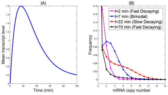
Figure 1.
The dynamics of the distribution by cross-talking pathways generated with min, min, min, min, and min. In (A), the observed mRNA average level behaves as up-and-down dynamics. In (B) the distribution transits from the decaying mode to the significant bimodality during a mediate time interval, and finally returns to decaying distribution.
Therefore, we guess that cross-talking regulation can generate these special dynamics compared with single-pathway regulation for some special parameters when the dynamic of the mRNA average level is up-and-down. What about the dynamical distribution by cross-talking pathways in the general condition?
Cross-talking pathways can modulate transcription dynamics of mean in two groups of fibroblast genes after TNF stimulation, and the dynamics of the two groups are both up-and-down [38]. In [39], they used the following two groups of data to fit the two groups dynamics in [38]:
Group I:
Group II:
Using these data to simulate the dynamics of distribution in the cross-talking pathways model, it is interesting to find that it generates similar dynamics to those in the special parameter region; see Figure 2.
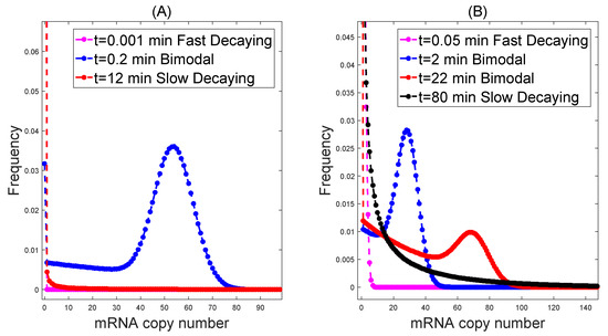
Figure 2.
Cross-talking pathways generate intermediate biomodal dynamical distribution with (A) h, h, h, , , h, h and (B) h, h, h, , , h, h.
5. Conclusions and Discussion
In this study, we calculated the expressions of the generating function and the probability mass function of the model for which the gene is activated by competitive cross-talking pathways. In a special parameter region, we successfully obtained the dynamic expression by simplifying some expressions firstly (Theorem 1) and deriving the expression in integral forms (Theorem 2). Together with transcriptional kinetic rates from yeast and mouse fibroblast genes, we found that, when the transcription average level regulated by the cross-talking pathways displays up-and-down dynamics, the corresponding mRNA distribution transits from the decaying mode to the intermediate bimodality as time develops, and finally returns back to the decaying mode (Figure 1 and Figure 2), which is not obtained [20].
In this work, the approach we present for calculating the of a cross-talking pathways model in a special parameter region only needs all parameters to be positive and finite. However, other current approaches to calculating require several parameters to be zero or infinity. This approach may be further developed for the general parameters condition. The dynamical scenario of decaying–bimodal–decaying distribution transition is different from the transcription of the mammalian c-Fos gene, which exhibits up-and-down dynamics of an average level, whereby the intermediate distribution takes unimodality [40]. However, such decaying–bimodal–decaying dynamical transitions matches exactly with the experimental data of yeast stress-response genes, which are regulated by a weak basal pathway under normal growth conditions, whereas they are strongly activated by the HOG-MAPK signaling pathway under acute stresses [15]. The theoretical result of this work is in good agreement with the experimental observations. Note that our observed mRNA distribution dynamics have not been generated by the models in which the gene is activated by a single pathway with multiple steps [37] or regulated by feedback loops [14]. Our work thus provides novel dynamics of mRNA distribution modulated by multiple signaling pathways.
Author Contributions
Conceptualization, C.Z.; methodology, C.Z.; software, Z.C.; formal analysis, Q.S.; data curation, Q.S. and Z.C.; writing—original draft preparation, Q.S. and C.Z.; writing—review and editing, Q.S. and C.Z. All authors have read and agreed to the published version of the manuscript.
Funding
This work was supported by the National Natural Science Foundation of China (Nos. 12101148, 12171113), the Natural Science Projects of Universities in Guangdong Province of China (No. 2020KTSCX237), the Natural Science Foundation of Guangdong, China (No. 2022A1515010242) and the Project of Guangdong Construction Polytechnic(No. ZD2020-02).
Institutional Review Board Statement
Not applicable.
Informed Consent Statement
Not applicable.
Data Availability Statement
All data included in this study are available upon request by contact with the corresponding author.
Acknowledgments
We thank Feng Jiao for his insightful suggestions.
Conflicts of Interest
The authors declare no conflict of interest.
References
- Cao, Z.; Filatova, T.; Oyarzun, D.A.; Grima, R. A stochastic model of gene expression with polymerase recruitment and pause release. Biophys. J. 2020, 119, 1002–1014. [Google Scholar] [CrossRef] [PubMed]
- Molina, N.; Suter, D.M.; Cannavo, R.; Naef, F. Stimulus-induced modulation of transcriptional bursting in a single mammalian gene. Proc. Natl. Acad. Sci. USA 2013, 110, 20563–20568. [Google Scholar] [CrossRef] [PubMed] [Green Version]
- Jing, X.; Loskot, P.; Yu, J. How does supercoiling regulation on a battery of RNA polymerases impact on bacterial transcription bursting? Phys. Biol. 2018, 15, 066007. [Google Scholar] [CrossRef] [PubMed] [Green Version]
- Larson, D.R. What do expression dynamics tell us about the mechanism of transcription. Curr. Opin. Genet. Dev. 2011, 21, 1–9. [Google Scholar] [CrossRef] [PubMed] [Green Version]
- Chen, L.; Lin, G.; Jiao, F. Using average transcription level to understand the regulation of stochastic gene activation. R. Soc. Open Sci. 2022, 9, 211757. [Google Scholar] [CrossRef]
- Jiao, F.; Sun, Q.; Lin, G.; Yu, J. Distribution profiles in gene transcription activated by the cross-talking pathway. Discret. Contin. Dyn. Syst. Ser. B 2019, 24, 2799–2810. [Google Scholar] [CrossRef] [Green Version]
- Jiao, F.; Tang, M. Quantification of transcription noise’s impact on cell fate commitment with digital resolutions. Bioinformatics, 2022; in press. [Google Scholar] [CrossRef]
- Jia, C. Kinetic foundation of the zero-inflated nagative binomial model for single-cell RNA sequencing data. SIAM J. Appl. Math. 2020, 80, 1336–1355. [Google Scholar] [CrossRef]
- Munsky, B.; Fox, Z.; Neuert, G. Integrating single-molecule experiments and discrete stochastic models to understand heterogeneous gene transcription dynamics. Methods 2015, 85, 12–21. [Google Scholar] [CrossRef] [Green Version]
- Cao, Z.; Grima, R. Analytical distributions for detailed models of stochastic gene expression in eukaryotic cells. Proc. Natl. Acad. Sci. USA 2020, 117, 4682–4692. [Google Scholar] [CrossRef] [Green Version]
- Cao, Z.; Grima, R. Accuracy of parameter estimation for auto-regulatory transcriptional feedback loops from noisy data. J. R. Soc. Interface 2019, 16, 20180967. [Google Scholar] [CrossRef] [PubMed]
- Jia, C.; Grima, R. Frequency domain analysis of fluctuations of mRNA and protein copy numbers within a cell lineage: Theory and experimental validation. Phys. Rev. X 2021, 11, 021032. [Google Scholar] [CrossRef]
- Peng, J.; Kocarev, L. First encounters on Bethe lattices and Cayley tree. Commun. Nonlinear Sci. Numer. Simul. 2021, 95, 105594. [Google Scholar] [CrossRef]
- Jia, C.; Grima, R. Dynamical phase diagram of an auto-regulating gene in fast switching conditions. J. Chem. Phys. 2020, 152, 174110. [Google Scholar] [CrossRef] [PubMed]
- Neuert, G.; Munsky, B.; Tan, R. Systematic identification of signal-activated stochastic gene regulation. Science 2013, 339, 584–587. [Google Scholar] [CrossRef] [Green Version]
- Chen, J.; Jiao, F. A novel approach for calculating exact forms of mRNA distribution in single-cell measurenments. Mathematics 2022, 10, 27. [Google Scholar] [CrossRef]
- Chen, L.; Zhu, C.; Jiao, F. A generalized moment-based method for estimating parameters of stochastic gene transcription. Math. Biosci. 2022, 345, 108780. [Google Scholar] [CrossRef]
- Jiao, F.; Sun, Q.; Tang, M.; Yu, J.; Zheng, B. Distribution modes and their corresponding parameter regions in stochastic gene transcription. SIAM J. Appl. Math. 2015, 6, 2396–2420. [Google Scholar] [CrossRef]
- Jiao, F.; Ren, J.; Yu, J. Analytical formula and dynamic profile of mRNA distribution. Discret. Contin. Dyn. Syst. Ser. B 2020, 25, 241–257. [Google Scholar] [CrossRef] [Green Version]
- Zhu, C.; Han, G.; Jiao, F. Dynamical regulation of mRNA distribution by cross-talking signaling pathways. Complexity 2020, 2020, 64026703. [Google Scholar] [CrossRef]
- Carey, L.B.; Dijk, D.V.; Sloot, P.M.A.; Kaandorp, J.A.; Segal, E. Promoter sequence determines the relationship between expression level and noise. PLoS Biol. 2013, 11, e1001528. [Google Scholar] [CrossRef] [PubMed] [Green Version]
- Golding, I.; Paulsson, J.; Zawilski, S.M.; Cox, E.C. Real-time kinetics of gene activity in individual bacteria. Cell 2005, 123, 1025–1036. [Google Scholar] [CrossRef] [PubMed] [Green Version]
- Raj, A.; Peskin, C.S.; Tranchina, D.; Vargas, D.Y.; Tyagi, S. Stochastic mRNA synthesis in mammalian cells. PLoS Biol. 2006, 4, e309. [Google Scholar] [CrossRef]
- Aguirre, A.; Rubio, M.E.; Gallo, V. Notch and EGFR pathway interaction regulates neural stem cell number and self-renewal. Nature 2010, 467, 323–327. [Google Scholar] [CrossRef] [PubMed] [Green Version]
- Lemaitre, B.; Hoffmann, J. The host defense of Drosophila melanogaster. Annu. Rev. Immunol. 2007, 25, 697–743. [Google Scholar] [CrossRef] [PubMed] [Green Version]
- Tanji, T.; Hu, X.; Weber, A.N.R.; Ip, T. Toll and IMD pathways synergistically activate an innate immune response in Drosophila melanogaster. Mol. Cell. Biol. 2007, 27, 4578–4588. [Google Scholar] [CrossRef] [PubMed] [Green Version]
- Jiao, F.; Lin, G.; Yu, J. Approximating gene transcription dynamics using steady-state formulas. Phys. Rev. E 2021, 104, 014401. [Google Scholar] [CrossRef]
- Sun, Q.; Jiao, F.; Yu, J. The dynamics of gene transcription with a periodic synthesis rate. Nonlinear Dyn. 2021, 104, 4477–4492. [Google Scholar] [CrossRef]
- Sun, Q.; Jiao, F.; Lin, G.; Yu, J.; Tang, M. The nonlinear dynamics and fluctuations of mRNA levels in cell cycle coupled transcription. PLoS Comput. Biol. 2019, 15, e1007017. [Google Scholar] [CrossRef]
- Sun, Q.; Tang, M.; Yu, J. Modulation of gene transcription noise by competing transcription factors. J. Math. Biol. 2012, 64, 469–494. [Google Scholar] [CrossRef]
- Yu, J.; Sun, Q.; Tang, M. The nonlinear dynamics and fluctuations of mRNA levels in cross-talking pathway activated transcription. J. Theor. Biol. 2014, 363, 223–234. [Google Scholar] [CrossRef] [PubMed]
- Iyer-Biswas, S.; Hayot, F.; Jayaprakash, C. Stochasticity of gene products from transcriptional pulsing. Phys. Rev. E 2009, 79, 031911. [Google Scholar] [CrossRef] [PubMed] [Green Version]
- Zhou, T.; Zhang, J. Analytical results for a multistate gene model. SIAM J. Appl. Math. 2012, 72, 789–818. [Google Scholar] [CrossRef]
- Evans, L.C. Partial Differential Equations, 2nd ed.; American Mathematical Society: Providence, RI, USA, 2010. [Google Scholar]
- Olver, F.W.J.; Lozier, D.W.; Boisvert, R.F.; Clark, C.W. NIST Handbook of Mathematical Functions, 1st ed.; Cambridge University Press: New York, NY, USA, 2010. [Google Scholar]
- Miller, C.; Schwalb, B.; Maier, K.; Schulz, D.; Dümcke, S.; Zacher, B.; Mayer, A.; Sydow, J.; Marcinowski, L.; Dölken, L.; et al. Dynamic transcriptome analysis measures rates of mRNA synthesis and decay in yeast. Mol. Syst. Biol. 2011, 7, 458. [Google Scholar] [CrossRef] [PubMed]
- Chen, Y.; Gong, Q.; Wu, Y.; Yan, H.; Hu, L.; Jiao, F. Dynamical mRNA distribution regulated by multi-step gene activation. AIP Adv. 2021, 11, 125015. [Google Scholar] [CrossRef]
- Hao, S.; Baltimore, D. The stability of mRNA influences the temporal order of the induction of genes encoding inflammatory molecules. Nat. Immunol. 2009, 10, 281–288. [Google Scholar] [CrossRef] [PubMed] [Green Version]
- Jiao, F.; Zhu, C. Regulation of gene activation by competitive cross talking pathways. Biophys J. 2020, 119, 1204–1214. [Google Scholar] [CrossRef] [PubMed]
- Senecal, A.; Munsky, B.; Proux, F.; Ly, N.; Braye, F.E.; Zimmer, C.; Mueller, F.; Darzacq, X. Transcription factors modulate c-Fos transcriptional bursts. Cell. Rep. 2014, 8, 75–83. [Google Scholar] [CrossRef]
Publisher’s Note: MDPI stays neutral with regard to jurisdictional claims in published maps and institutional affiliations. |
© 2022 by the authors. Licensee MDPI, Basel, Switzerland. This article is an open access article distributed under the terms and conditions of the Creative Commons Attribution (CC BY) license (https://creativecommons.org/licenses/by/4.0/).