Abstract
The identification and estimation of trends in hydroclimatic time series remains an important task in applied climate research. The statistical challenge arises from the inherent nonlinearity, complex dependence structure, heterogeneity and resulting non-standard distributions of the underlying time series. Quantile regressions are considered an important modeling technique for such analyses because of their rich interpretation and their broad insensitivity to extreme distributions. This paper provides an asymptotic justification of quantile trend regression in terms of unknown heterogeneity and dependence structure and the corresponding interpretation. An empirical application sheds light on the relevance of quantile regression modeling for analyzing monthly Central England temperature anomalies and illustrates their various heterogenous trends. Our results suggest the presence of heterogeneities across the considered seasonal cycle and an increase in the relative frequency of observing unusually high temperatures.
JEL Classification:
C02; C14; C18; C22; Q54
1. Introduction
The current phase of rapidly accelerating impacts of global warming reveals many immediate effects on direct and indirect threats to global health and clearly illustrates the role of human activities (e.g., [1,2]). Recently, the International Panel on Climate Change [3] reported unprecedented increases in global surface temperature over the last four decades since the start of geo-referenced systematic climatological records in 1850—with larger increases for land- than sea-surface temperatures. Substantial increases in mean temperatures across the world and heterogeneity in temperature increases across months are noted in Vogelsang and Franses [4], who emphasize that especially winters are warming in the northern hemisphere. King et al. [1] document substantial warming in the Central England Temperature (CET) time series for 2014 based on simulated and observed datasets and provide evidence for a human-induced increase in the relative frequency of observing record high temperatures. King [5] extends their previous analysis beyond the univariate approach and provides a proxy for the local response to global warming by modeling local temperature as a nonlinear parametric function of global temperature. Rivas and Gonzalo [6] provide a definition of global warming and trending time series and present evidence for warming based on the CET and global temperature time series.
The properties of climatologic time series have been frequently studied in the literature and the related findings fuel an ongoing debate about the analysis and attribution of trends (see, e.g., [7,8], for recent summaries and discussions). When investigating the properties of climatologic time series, seasonality is typically filtered in a first step, as it may frustrate diagnostic tests and complicate inference (e.g., [9], in the context of long range dependence and structural breaks). After filtering the seasonal annual cycle, Gao and Franzke [10] test temperature series for the presence of long range dependence. Proietti and Hillebrand [11] conduct a series of univariate (and multivariate) stationarity (and cointegration) checks against various alternatives and find evidence of nonstationarity. Their findings are in line with He et al. [12]. Among others, Fomby and Vogelsang [13], Barbosa [14], and Franzke [15] discuss previous studies suggesting that temperature series are mean stationary and exhibit long range dependence. While such dynamics do not generate trends in the long run (e.g., thousand years or longer), series such as the CET ranging over a few hundred years may exhibit stochastic trends. Whether such trends are deterministic or stochastic and due to short run or long run dependence has been investigated intensively (e.g., [4,11,16]).
Koenker and Schorfheide [17] investigate curvature in temperature trends in greater detail. They discuss an upward trend in global Hansen-Lebedeff temperatures [18] between 1880 and 1940 and after 1965, and identify a trend break in a period of decreasing temperatures between 1940 and 1965. An important challenge in the analysis of hydrologic and climatologic processes is the delicate interplay of nonlinearities, temporal dependence, bimodality, and heterogeneity (e.g., [5,17,19,20,21,22,23]). Rial et al. [24] provide potential explanations of the mechanisms underlying the climate system such as the superposition of shift and trends in long-term and short-term dynamics, ocean atmosphere interactions, and feedback effects from the carbon-cycle. Koenker and Schorfheide [17] suggest to broaden the perspective of analysis beyond the common practice of modeling the deviations around deterministic trends for the conditional mean temperature using ARIMA (autoregressive integrated moving average) processes. They propose the use of conditional quantiles as “serial correlation may be due to a variety of mechanisms that could plausibly effect year-to-year changes” in temperature and climatic conditions in general (e.g., [25]). As a consequence, in recent contributions to statistical modeling of temperature series, the method of quantiles introduced by Koenker and Bassett [26] plays a major role to define and identify anomalies (e.g., [27,28]).
The presence of seasonal trends has been discussed for climatologic time series by Colman [29], who argues that sea-surface temperature anomalies may drive seasonal trends in temperature series, which entails important consequences for ecologic policy (e.g., [30]). Recently, He et al. [12] emphasized that seasonal trends are difficult to model and forecast due to time-varying patterns in their components. In what follows, we avoid the perils of applying a particular approach to filter seasonality and use the assumption of cyclostationarity (e.g., [31]) in a quantile trend regression (QTR) framework. Cyclostationarity is based on the literature on periodically autocorrelated processes (e.g., [32]) and assumes that trend patterns vary cyclically over time. As a consequence of this, temperature can be understood as a stationary process fluctuating around a deterministic trend component. Thus, by splitting up the original series into S non-seasonal subseries, where S corresponds to the length of the seasonal cycle, the estimating equations in our QTR framework can then be decomposed into two parts which are allowed to vary over the temperature distribution: the conditional temperature quantile estimated by a trend polynomial and a stationary colored noise process. We provide a detailed derivation and discussion of the assumptions underlying the QTR model and show the asymptotic normality of the QTR estimator. Additionally, we analyze temperature time series which are known to be crucial factors in models explaining morbidity and mortality and which are frequently used as predictors for other entities in epidemiology, climatology, ecology and economics.
The paper is structured as follows. Section 2 introduces a sketch of a baseline mathematical model and from this derives the QTR model, its assumptions, and asymptotic properties. Section 3 provides an overview of the CET anomaly data, illustrates the relevance of quantile regression for analyzing anomalies, and summarizes and discusses the modeling results. Section 4 provides concluding remarks.
2. Methods
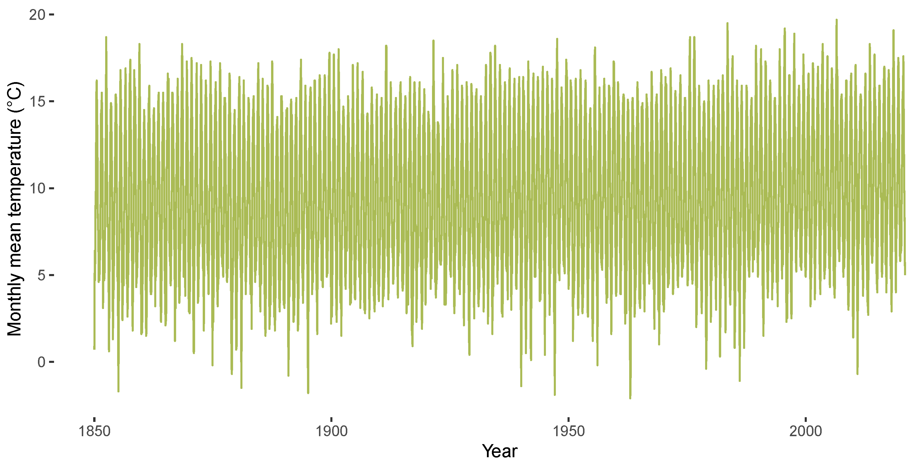
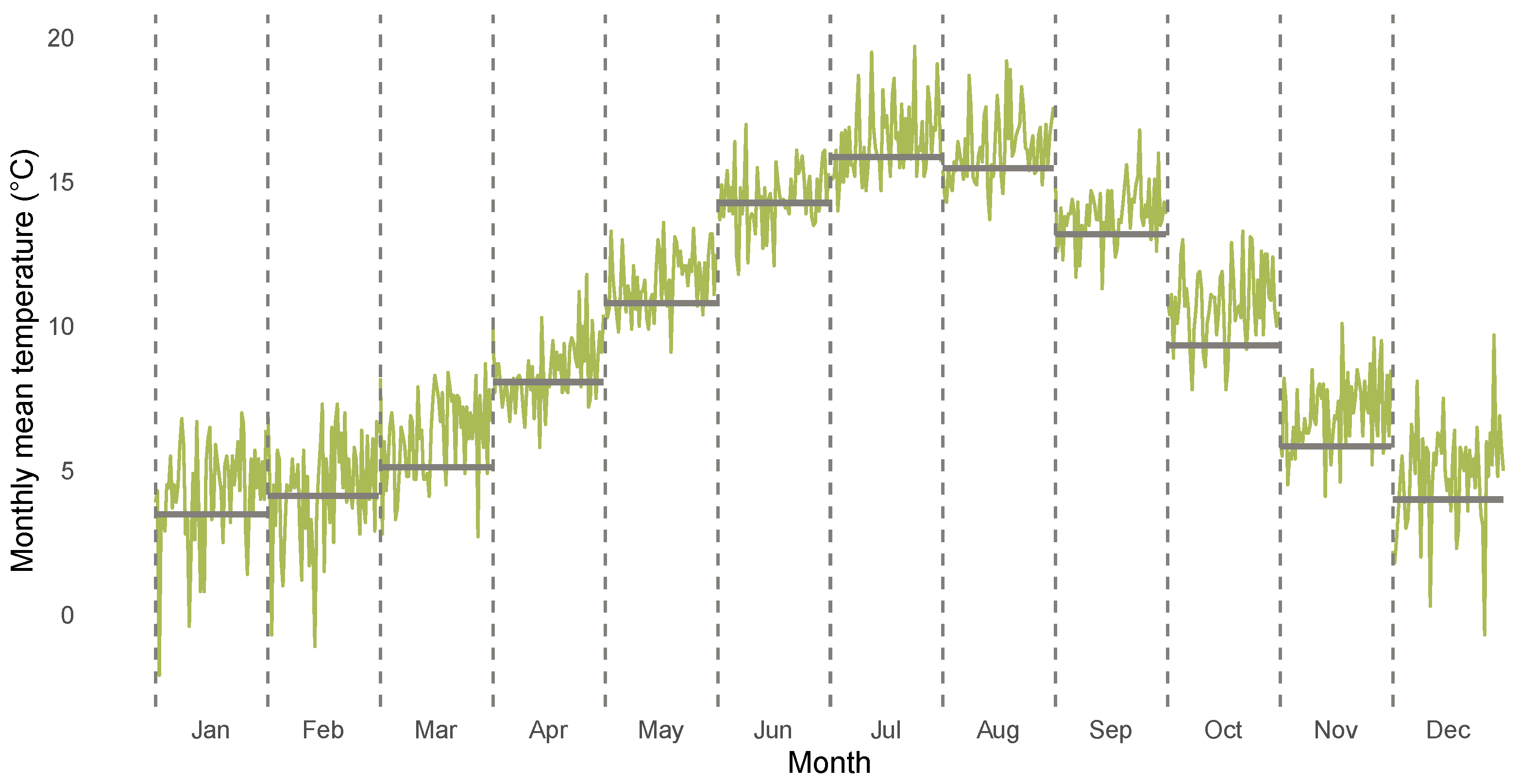
Figure 1 and Figure 2 highlight stylized facts of the CET data from January 1850 to December 2020 analyzed in the empirical section of the paper. Figure 1 shows the CET data, Figure 2 illustrates the corresponding annual mean temperatures. A season plot for the CET data is given in Figure 3, which includes the monthly mean temperature for each month from 1850 until 1900 via the grey horizontal lines. The latter figure illustrates the presence of heterogeneity in the respective monthly levels of temperature and also in the month-specific trajectories of temperature. The figures illustrate the generic nonlinearity and nonstationarity often found in environmental and hydroclimatic processes due to seasonal cycles or trend patterns. The decomposition of time series into trend and seasonality is the starting point for our modeling framework. We thereby address the requirements identified by Proietti and Hillebrand [11] that the temperature exhibits month-specific variation, dependence and trend patterns, while a global trend affects all months in a potentially different way. We will address this problem by using an approach similar to the modeling of periodically correlated sequences (e.g., [32]).
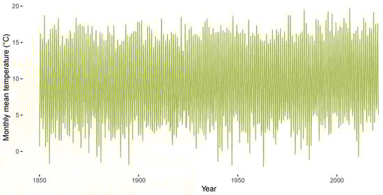
Figure 1.
CET data from 1850 until 2020.
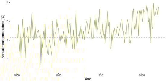
Figure 2.
Annual mean temperature in Central England from 1850 until 2020. Dashed grey line represents annual mean temperature during years 1850 until 1900.
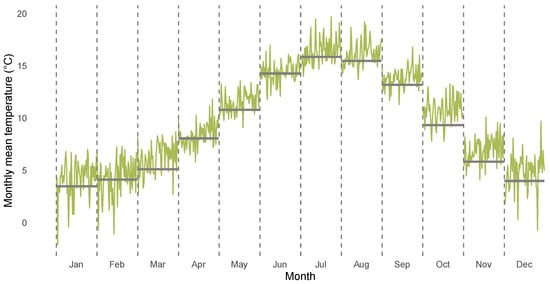
Figure 3.
CET data for each month from 1961 until 2020. From left to right, months January to December are displayed over the years. Grey lines indicate monthly mean temperature from 1850 until 1900. Different months separated by dashed vertical lines.
2.1. Baseline Model
Let be a complete probability space and, following Koenker and Schorfheide [17], consider temperature data to be an -measurable scalar random sequence. Further assume that this process has a single cyclical component due to the annual season . This assumption implies that potential nonstationarities at seasonal position s (i.e., for each of the months in our application) can only be generated by trend components (see [12] for a discussion in autoregressive models). Our approach deviates from the concept of periodical correlation in the Hilbert space of random variables with finite second moment, as we do not require the existence of any moments of the random processes constituting the estimating equation. However, we will exploit that the quantile regression loss function defined below belongs to the class of absolutely continuous (on every interval) functions with right-hand-derivative , which is a function of bounded variation (e.g., [33], Section 2.3).
Employing a common notation for seasonal time series (e.g., [12,34]) we denote the time index t as where is a new (annual) time index and consider a realization with sample size . We assume that the data are generated according to
where is an unknown function continuous in , which depends on unknown but fixed season-specific parameters , the row vector contains known and deterministic covariates depending on n, and is an error process.
We assume that the set of control variables does not vary over the seasons. Then, following Yang and Tschernig [34], the task of variable selection and parameter estimation has to be carried out for each month and corresponding data set
The Weierstrass approximation theorem states that we can approximate
In the semiparametric context of model (1), we assume a polynomial regression design
The baseline example in our data analysis is to assume that month-specific temperature series are generated by linear deterministic trends and additive, stationary and weakly dependent errors .
Example 1.
Our empirical analysis of the CET data investigates temperature anomalies over the last 60 years from 1961 to 2020. Thus, , , and the effective sample size is . For convenience we consider the index . A simple special case for a month-specific trend equation is the linear trend equation
Using the QTR model, we will estimate for each month s, , and various quantiles , . Least squares based diagnostic testing, estimation, and inference of temperature trend regressions (4) have been discussed among others by Fomby and Vogelsang [13], Fatichi et al. [16], Barbosa [14], and in detail by Mudelsee [23].
2.2. Quantile Trend Regression
Instead of a least squares based trend modeling of the month-specific annual average increase of temperature data over time, we employ quantile regression. The resilience of quantile regression to extreme values in the temperature distribution allows robust estimation of annual median increases but also other non-central aspects of the temperature processes. As a consequence, the QTR estimator introduced in this chapter allows to draw inferences on trend patterns and their variation over the temperature distribution. We derive the asymptotic normality of the QTR estimator under primitive assumptions. Our argumentation is similar to Pollard [35], Fitzenberger [36], and Koenker [37], but builds on the weaker assumptions and corresponding results of Oberhofer and Haupt [38,39,40].
2.2.1. Basic Structure of a Quantile Regression Model
Our goal is to study season-specific trend patterns and investigate their heterogeneity over the temperature distribution. For this purpose we formulate a QTR model for each seasonal position s. For the sake of simplicity we will omit the index s whenever the context is clear. Using annual data, we assume that the temperature processes are generated according to the QTR equation
where , , are known deterministic design vectors, and the true parameter is an inner point of a compact subset of . The unknown parameter vector is estimated by the minimizer
where and the conditional quantile is the optimal predictor of Y under quantile regression loss [26]
where is the usual indicator function. By we denote the distribution of , by the joint distribution of for , and employ the usual normalization in quantile regression:
(A1) , , ∀i.
Starting from these core components of a quantile regression model, we motivate further assumptions required to derive the asymptotic normality of the QTR estimator. Due to the different growth rates of the components in the polynomial design (3), a normalization has to be applied (see [41], Ch. 7.2, for a detailed discussion in the case of least squares regression). Define
where is a nonsingular diagonal matrix with positive elements for and for large enough N. The normalization (8) has to ensure that the elements of are Cesàro-summable (e.g., [33]).
Example 2.
For the cubic polynomial trend model employed in Franzke [28], is of order 1, is of order , is of order , and is of order .
(A2) The vectors are deterministic and known and for some real number M, , for , and all N.
For our asymptotic analysis we re-write the argument of (6) according to (5) as
with local parameters and . Following Huber [42], we can then write the QTR objective function as
with summands
Then, under suitable assumptions (e.g., [37], Ch. 4, for the assumption of independent but not identically distributed random variables) the limiting distribution of can be derived from that of . If is the minimand of the scalar random variable , then the QTR estimator of is given by
Remark 1.
In least squares regression, asymptotic analysis relies on the twice continuously differentiable loss function and local uniform approximation of . As this approach is not feasible in quantile regression, we have to approximate by a sufficiently smooth function . Due to its inherent smoothing, the expectation is a suitable choice, whenever a uniform LLN can be established such that
for in a compact subset of . Further elaboration is beyond the scope of this paper (see, e.g., [40], Lemma 2C), but we will get back to (15) in Remark 2 below and then analyze the asymptotic behaviour of in Lemma 2.
Knight [43] suggests a useful decomposition of , which allows to study its asymptotic behavior by examining that of its partial sums separately. Knight’s identity is given by
where the second summand in (16) is defined as
where
is the right-hand-derivative of (7), and
The first summand in (16) is defined as
The definition of summands implies (e.g., [44], Lemma 3.1)
As a consequence, every moment of exists for finite . Then, due to assumption (A1), , and it holds that
and
2.2.2. Modeling the QTR Dependence Structure
In the case of independence, the previous arguments suffice to describe the relevant properties of and . In this case we obtain and for . In the case of dependence, we require a suitable assumption concerning the asymptotic behavior of . From the definition of in (19) follows
where can be interpreted as local measures of dependence, defined as
Define the matrix with generic elements (25). Further define the design matrix with rows defined in (3) and in analogy to (8). Then
Given (24) and (26), we can derive the limiting distribution of by introducing a suitable assumption on the limiting behavior of defined in (25).
(A3) Let , . Then, of size , where .
As has been pointed out by Oberhofer and Haupt [39], only the properties of the Bernoulli process and the local behavior of the distribution functions and densities in the neighborhood of and , respectively, are essential for dependence in quantile regression. Assumption (A3) implies that ) is strong mixing of size , where . Let denote the sigma-algebra generated by . Then, , as r approaches infinity, where and . For mathematical convenience it is typically assumed that the error process is strong mixing (e.g., [40]), as there exist numerous examples in time series analysis on mixing processes and a rich mathematical theory (e.g., [33,45,46,47]).
Lemma 1.
Under assumptions (A1), (A2), and (A3), converges in distribution to , where is normally distributed with mean zero and covariance
Proof.
Assumption (A3) implies that is strong mixing of size , where , with mixing coefficient . Since is near-epoch dependent (-approximable) on , we can apply Theorem 10.2 in Pötscher and Prucha [47]. Then, the assertion follows from (26) and upon application of the Cramér-Wold device [48]. □
Instead of relying on the existence of moments as in least squares regression, in quantile regression we require that has a density (with respect to Lebesgue measure), and that is informative at the conditional quantile we want to estimate.
(A4) For some , the density of exists for every i and , is uniformly continuous in i at , and .
Define the diagonal matrix with elements , . Then, in our main result we show that
converges to the asymptotic covariance matrix of the QTR estimator as . Expression (27) reveals that dependence and heterogeneity can be treated separately in quantile regressions under non-iid settings:
corresponds to covariances and
to variances. This discussion reveals the need for further assumptions on the dependence structure guaranteeing the existence of (27) as .
(A5) For some , the density of exists for , , and , is continuous at uniformly in i and j, and , where , and the supremum is taken over .
(A6) converges for to a matrix Σ.
(A7) converges for to a non-singular matrix .
If the errors are independent, and the sum in assumption (A5) is equal to zero for all N. Then assumptions (A4) and (A5) are implied by the existence of in the neighborhood of , and the continuity of at . Assumption (A5) can be interpreted as an infinitesimal weak dependence condition similar to the “dependence index sequence" of Castellana and Leadbetter [49]. Assumptions (A6) and (A7) ensure the existence of the covariance matrix (27) in the limit. While the dependence structure is contained in assumption (A6), the heterogeneity is captured by assumption (A7). Note that a too strong dependence hinders convergence in (A6). Obviously, if the limit of the matrix is singular, then the limiting distribution of is singular, too.
2.2.3. Main Result
The proof of our main result rests on Lemma 1 and two additional Lemmas. Lemma 1 derived the limiting distribution of . Lemma 2 establishes that (see Remark 1) converges uniformly for in a compact subset of to . Lemma 3 establishes that converges uniformly to 0 for in a compact subset of .
Remark 2.
In our derivations we assume and apply assumptions (A4) and (A5). Hence we implicitly assume the consistency of . The ULLN (15) required for this can be derived from (i) a weak LLN for weakly dependent sequences using the -approximability of by (see [47], Theorem 6.2, and the proof of Lemma 1) and (ii) stochastic equicontinuity of the (e.g., [33], Section 21.3). Then, weak consistency of in the QTR model can be established using the arguments in (Oberhofer and Haupt [40], Lemma 2C, Theorem 1) or (Fitzenberger [36], Theorem 2.2).
Lemma 2.
Under assumptions (A2), (A4), and (A7), converges for to . The convergence is uniform for in a compact subset of .
Proof.
For , from (20) and assumption (A4) follows from the mean value theorem
Apply an analogous argumentation for . From assumption (A2) follows . Finally, due to assumption (A4),
and the assertion follows from assumption (A7) (e.g., [37], Theorem 4.1). □
Lemma 3.
Under assumptions (A2), (A4), and (A5), . The convergence is uniform for in a compact subset of .
Proof.
For , , and ,
An analogous argumentation applies for , and all other cases. Then,
The expression on the right hand side is bounded from above by
Thus, according to assumptions (A5) and (A2), the left hand side of (30) tends to zero as . Analogously, for ,
Then, the assertion follows from assumptions (A2) and (A4). □
Theorem 1.
Under assumptions (A1)–(A7), the minimizing value of converges in distribution to a normal distribution with mean zero and covariance matrix .
Proof.
According to Lemmas 1–3 and assumption (A6), converges for in distribution to
with minimizing value . The limiting value can be interpreted as the limit of a second order Taylor expansion of . The convergence in distribution of the minimizing value to requires the convexity of [35] and the uniform convergence results established in our Lemmas for in a compact subset of . □
3. Data and Results
This section provides descriptives for the CET data from 1850 until 2020 used for fitting the QTR models and summarizes the modeling results. All temperatures are measured in Celsius degrees (C). The CET time series is recorded by a network of monitoring stations (see [1], Figure 1a for a visualization of the locations) and designed to represent the climate of the English Midlands. The time series decomposition of the CET time series and the description of its key characteristics has received considerable attention in the literature (see, e.g., [1,4,11,12,15,29,50,51] for contributions over the past two decades).
All computations and visualizations were obtained with the statistical software R version 4.1.1 [52] using the addon packages quantreg [53], forecast [54], ggplot2 [55], and gridExtra [56]. Data and code (Supplementary Materials) is available from an online repository [57].
3.1. Descriptives for CET Anomalies
In the following analysis of the CET data, we focus on monthly temperature anomalies (hereafter anomalies). To construct the anomalies, we first compute mean monthly temperatures for each month over the years 1850 until 1900 . This time period is generally considered to approximate pre-industrial levels and facilitates comparability of our results for Central England with other regions due to the availability of gridded surface temperature records (see, e.g., Chapter 3, p. 20 in [3], and the references cited therein). The anomalies are obtained by subtracting from the CET data for the years 1961 until 2020 shown in Figure 3. Table 1 displays for each month of the years 1850 until 1900 (first row), mean monthly temperatures for the years 1961 until 2020 (second row) and the anomalies . Note that all displayed anomalies are positive.

Table 1.
Mean monthly temperatures (C) for years 1850 until 1900 (first row) and years 1961 until 2020 (second row). The third row displays corresponding anomalies for years 1961 until 2020.
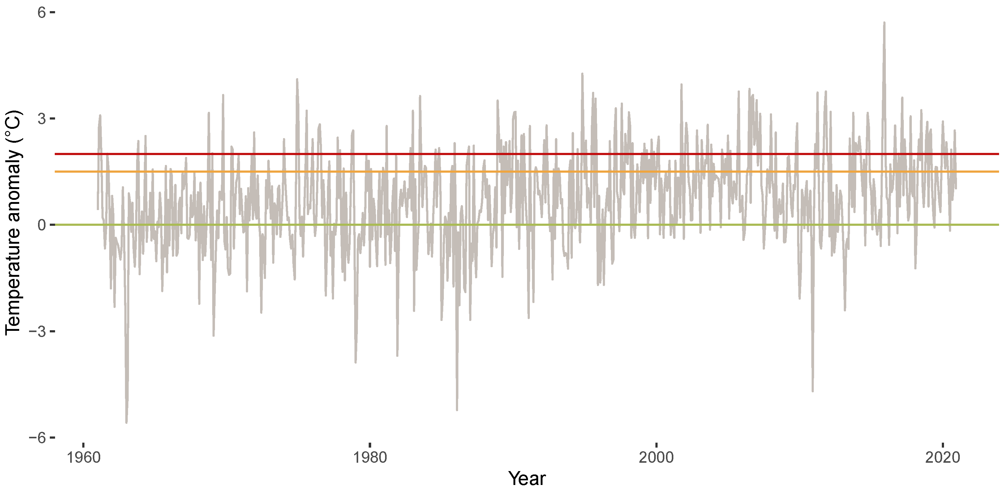
Figure 4 shows the time series plot of the anomalies for the years 1961 until 2020. Similar to King et al. [21], we include threshold lines for 0 C (green), 1.5 C (orange), and 2 C (red) in all visualizations of the anomalies (for detailed reasoning and brief summaries, see [58,59,60]).
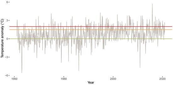
Figure 4.
Anomalies for years 1961 until 2020 (grey line). Horizontal lines indicate anomalies of 0 C (green), 1.5 C (orange), and 2 C (red).
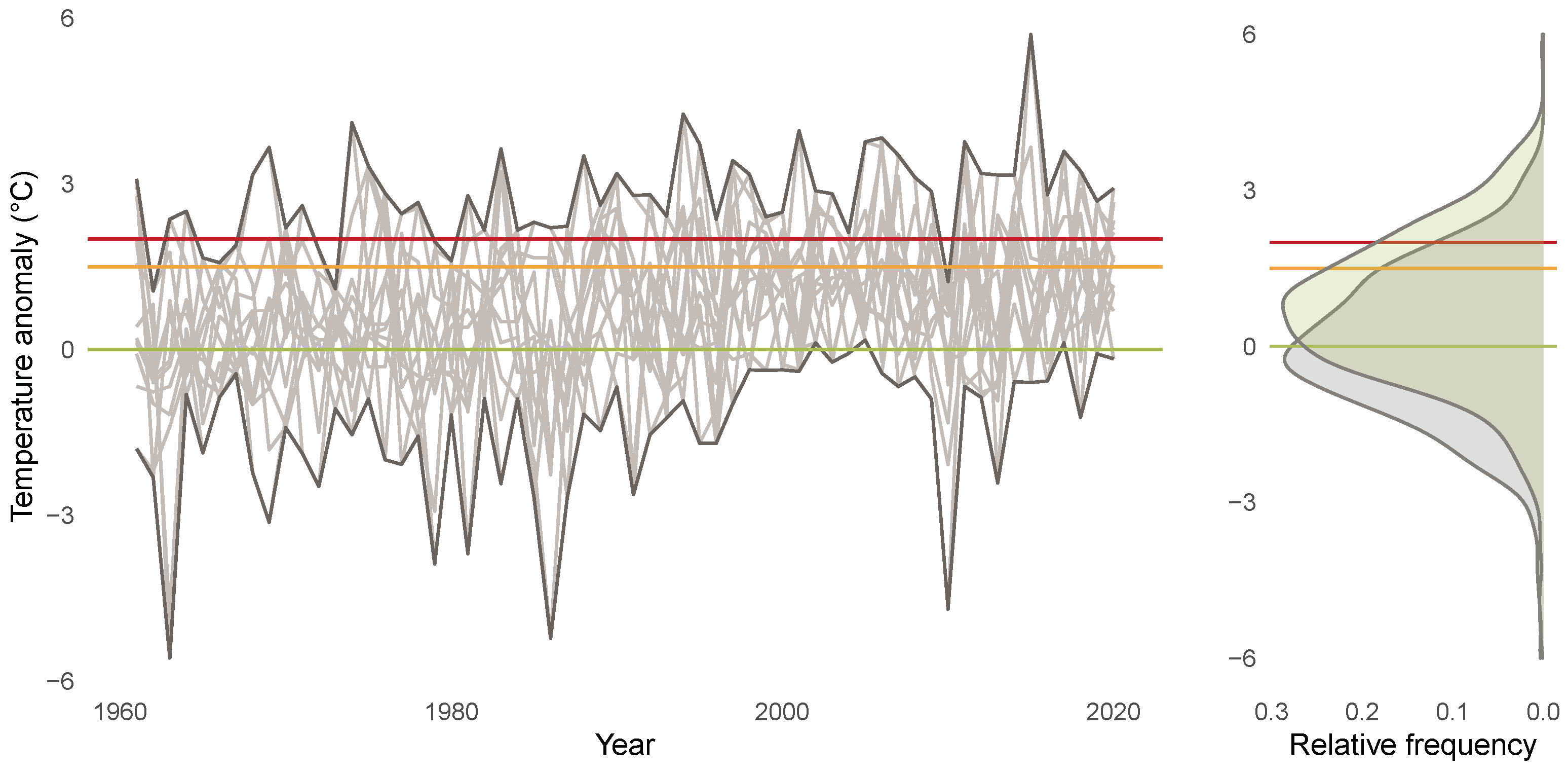
Figure 5 visualizes the anomalies for the different months (left display) and the empirical density of the anomalies (right display). Each line in the left display visualizes one time series of anomalies for a particular month from Figure 4. The anomalies show an upward trend and most of the anomaly time series are located above the green line after the year 2000. The empirical density of the anomalies shows a location shift when comparing the years 1961 until 2020 (green area) to the years 1850 until 1900 (grey area), with a mean anomaly during the years 1961 until 2020 of 0.71. Note that the empirical density that an anomaly exceeds 2 C (marked by the red line) triples for the years 1961 until 2020 compared to the years 1850 until 1900.

Figure 5.
Anomalies for years 1961 until 2020 (left display), where each line represents anomalies for one month. Right display shows empirical densities of anomalies for years 1850 until 1900 (grey) and 1961 until 2020 (green). Horizontal lines indicate anomalies of 0 C (green), 1.5 C (orange), and 2 C (red).
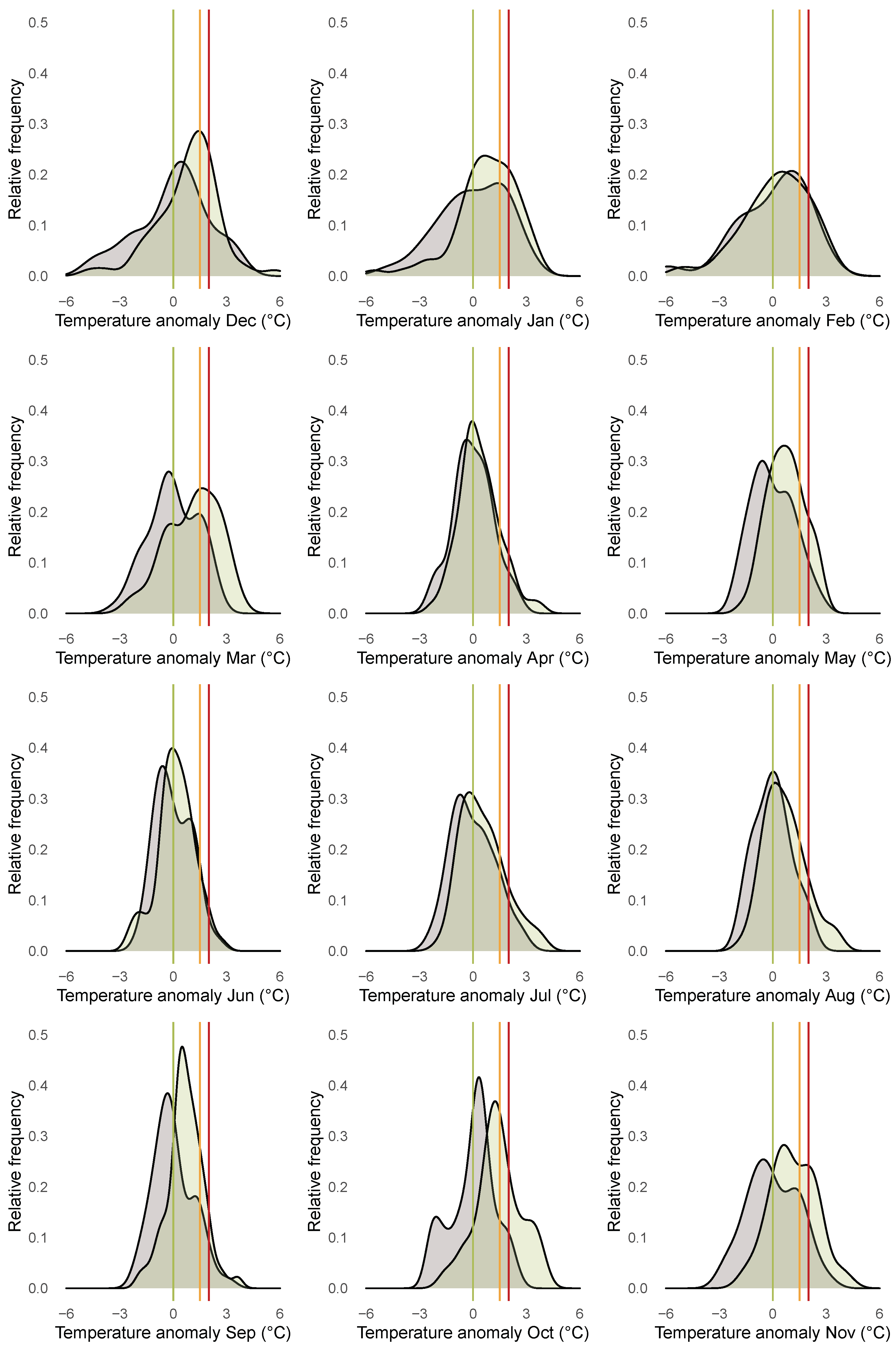
To obtain a more complete picture of potential heterogeneities across the different months, we investigate the months separately. Figure 6 shows boxplots for the anomalies for each month over the years 1850 until 1900 (grey) and the years 1961 until 2020 (green). The different boxplots indicate substantial heterogeneities across the months with respect to the dispersion of the distribution of the anomalies. The dispersion is higher for the winter months compared to the summer months. Additionally the boxplots illustrate that location shifts in the anomalies are more pronounced for the autumn and winter months compared to the other months. Figure 7 shows the empirical densities for the anomalies from January 1850 until December 1900 (darkgrey) and from January 1961 until December 2020 (green) separately for each month. Starting from December in the top left corner to November in the bottom right corner, the rows of the figure represent the winter (first), spring (second), summer (third), and fall (fourth) months. The figure indicates the presence of a location and scale shift in the conditional distribution of temperature anomalies, which varies across the different months and is more pronounced in fall and winter.
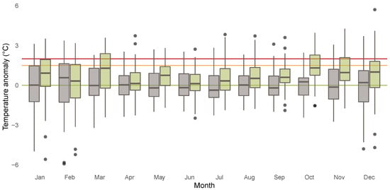
Figure 6.
Boxplots for anomalies for years 1850 until 1900 (grey) and 1961 until 2020 (green) for each month. Horizontal lines indicate anomalies of 0 C (green), 1.5 C (orange), and 2 C (red).
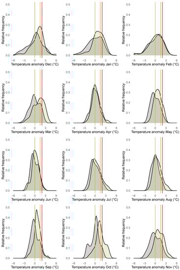
Figure 7.
Empirical densities of anomalies plotted for each month from January 1850 until December 1900 (grey) and from January 1961 until December 2020 (green). Vertical lines indicate anomalies of 0 C (green), 1.5 C (orange), and 2 C (red).
3.2. Relevance of Quantile Regression for Analyzing Anomalies
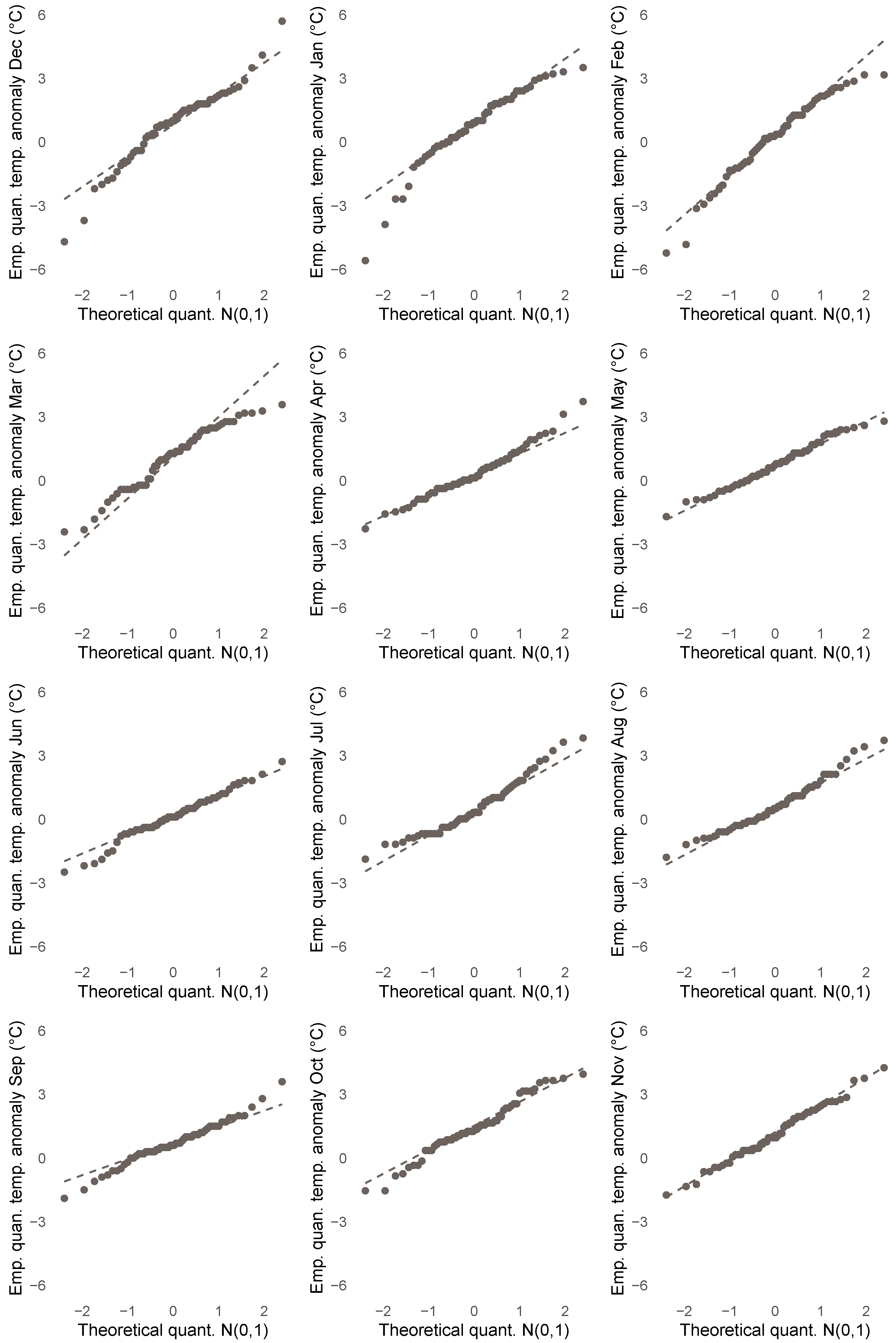
In this subsection, we highlight properties of the anomalies that indicate that quantile regression analysis is more appropriate in this case compared to least squares analysis. Figure 8 displays QQ-plots of the sample quantiles of the anomalies (ordinate) for each month against the theoretical quantiles of the standard normal distribution (abscissa) and reveals that the empirical anomaly distributions appear “almost normal” only for months May and November, while there are a number of deviations from normality in all other months. In particular, we observe evidence of skewness (left: January, February, June; right: April, July, August) and outliers (December, January, February, March), which may heavily influence the accuracy of least squares based statistics. Additional evidence of fat tails (September, October, December) may trouble the existence of moments.
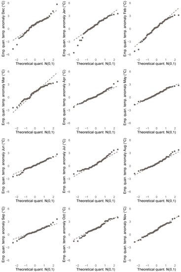
Figure 8.
Sample quantiles of anomalies for each month from January 1961 until December 2020 (ordinate) and theoretical quantiles of standard normal distribution (abscissa). Dashed grey line connects points constituted of respective 0.25%- and 0.75%-quantiles.
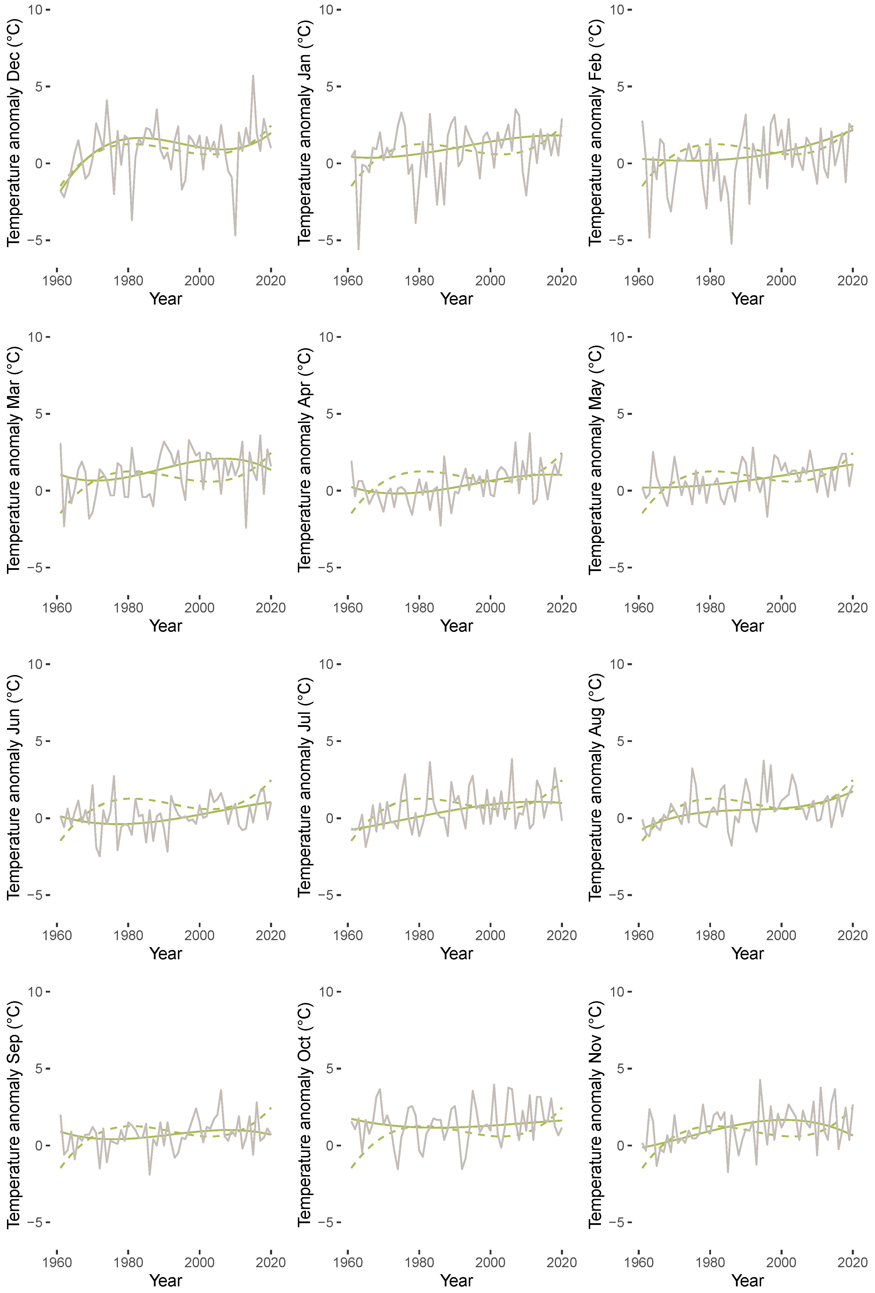
Figure 9 displays estimated mean versus median trends of anomalies for each month starting from December (top left) to November (bottom right). The trend regressions were fitted by employing a polynomial of degree three in a quantile regression with (solid green line) and a least squares regression (dashed green line). The figure highlights that there are considerable differences between the conditional mean and the conditional median for all months except December. In particular, skewness and extreme values lead to a much more wiggly behavior of the mean trend compared to the median trend.
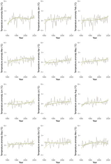
Figure 9.
Estimated trend polynomial of degree three by quantile regression (; solid green line) and least squares regression (dashed green line) for anomalies for each month from January 1961 until December 2020 (grey lines).
3.3. Results of QTR Estimation
In the sense of our mathematical model in Equation (1), we analyze all monthly CET anomaly time series separately (e.g., [4,34,61]) by fitting a QTR model as defined in Equation (5) for time series of monthly temperature anomalies to capture month-specific patterns of trend and heterogeneity. Similar to Franzke [15], we use a low-order polynomial for trend modeling and fix the order of the polynomial regression design given in Equation (3) to :
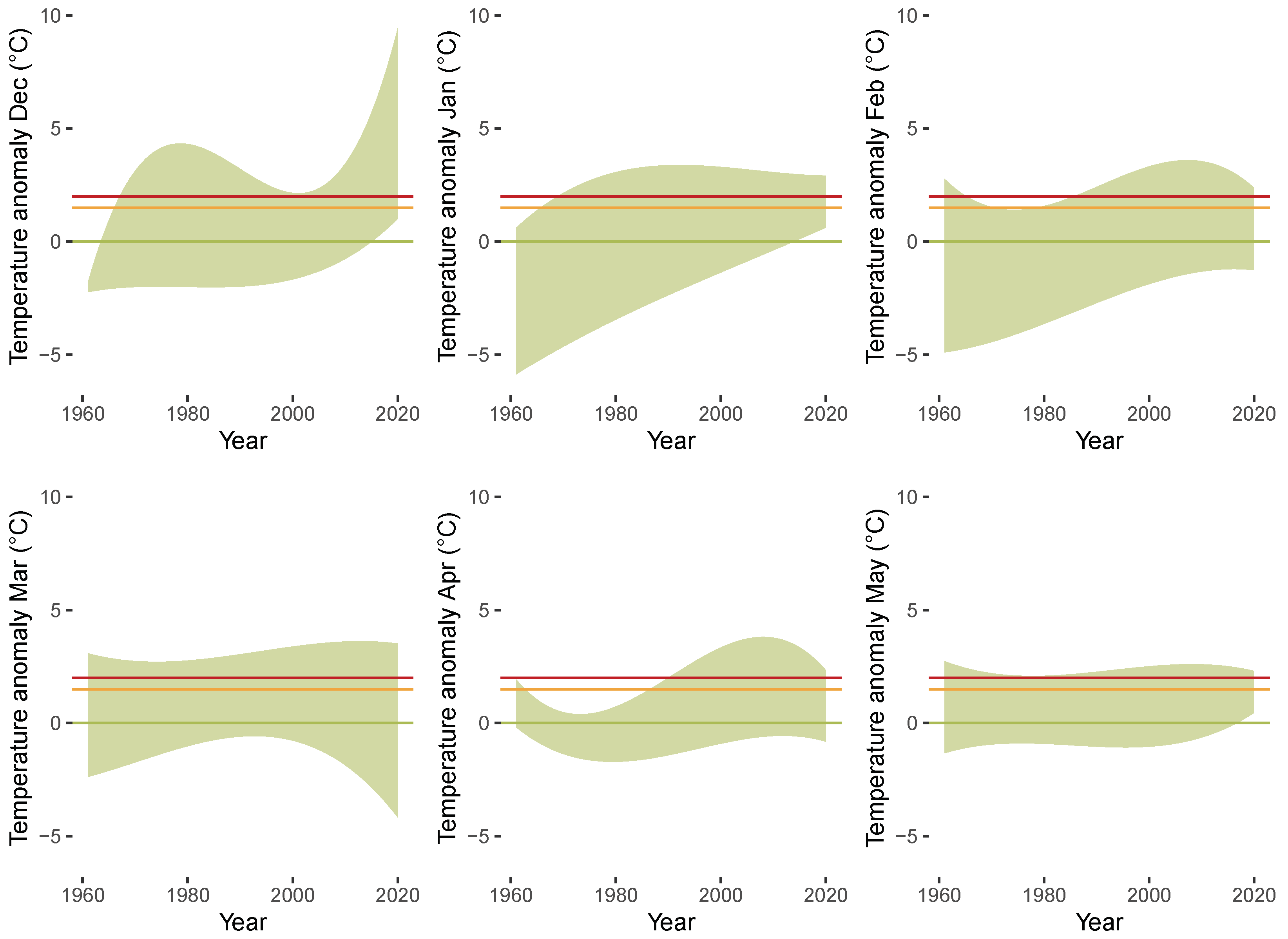
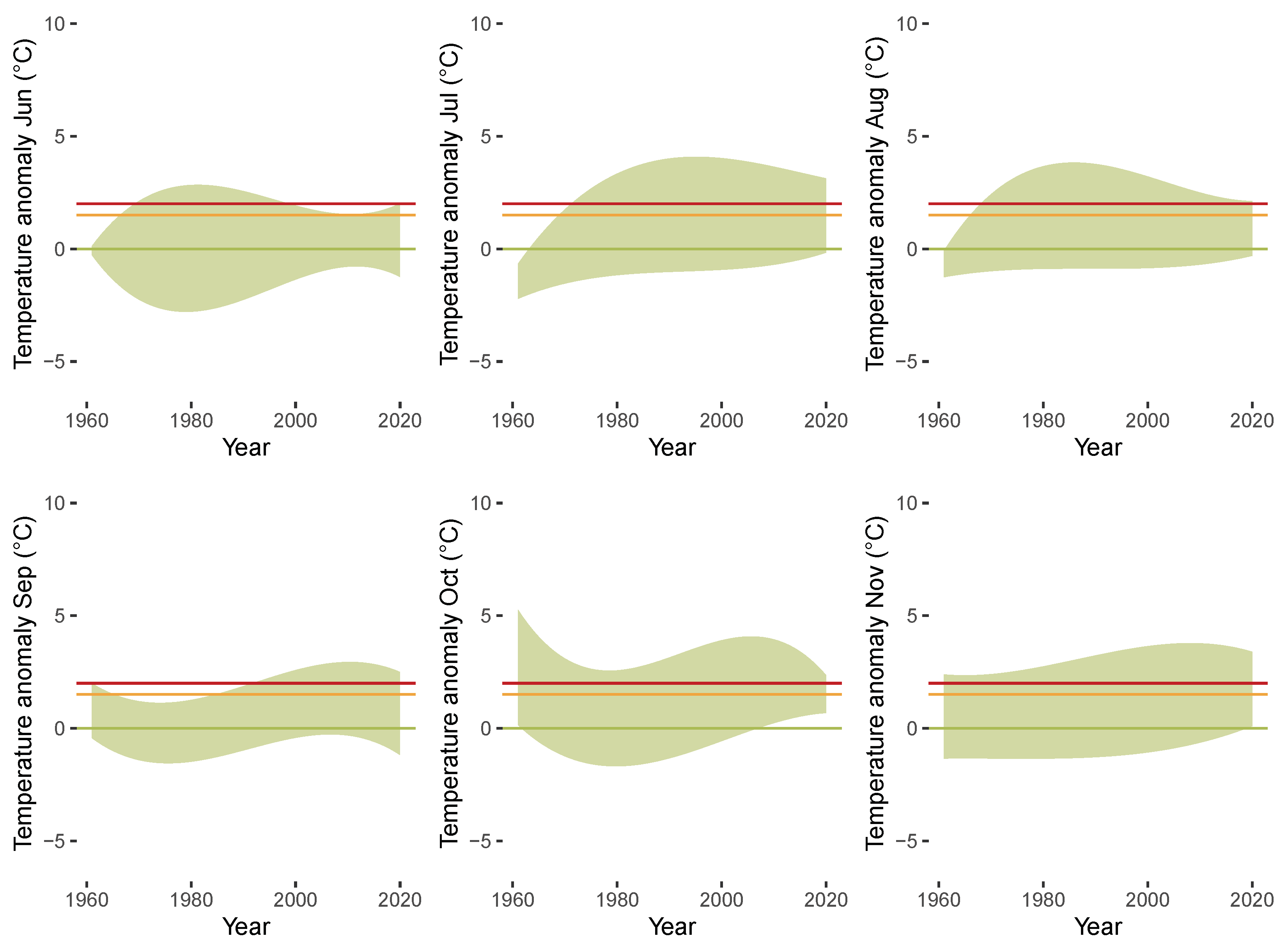
Figure 10 illustrates the QTR models fitted to the anomalies. Each display represents the QTR model fit to a particular month from December (top left) to November (bottom right). In our further analysis of the CET data, we focus on hot and cold extremes. Following Franzke [28], we define the quantile as threshold for hot extremes and the quantile as threshold for cold extremes. Visualizations based on the exceedance of such thresholds can be found, among others, in Mudelsee [62] and Dissanayake et al. [63]. Alternatively, Glick [64] considers the maximum and minimum as thresholds for hot and cold extremes. The area between the estimated quantile trend curves for hot () and cold () extremes is marked in green. The estimates indicate that there are substantial heterogeneities with respect to two dimensions: Across the quantiles (when contrasting the lines that bound the green area above and below for each display) and across the monthly seasonal cycle (when contrasting the green areas over the different displays). Upward trends in the anomalies are visible for almost all months, as larger fractions of the areas move above the zero line over time. The divergence between the hot and cold quantiles is larger for winter months compared to summer months. Overall, our results are in accordance with earlier literature, which provided evidence for global warming and trending in temperature time series and noted heterogeneity across the different months (e.g., [4,6,28]).
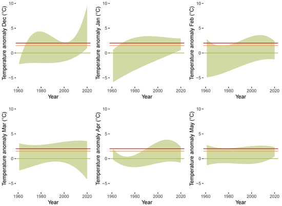
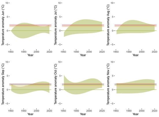
Figure 10.
Anomalies for each month from January 1961 until December 2020. Green shaded area colors region between QTR models for hot ( quantile) and cold ( quantile) extremes. Horizontal lines indicate anomalies of 0 C (green), 1.5 C (orange), and 2 C (red).
4. Concluding Remarks
We propose a model for season-specific trends motivated by cyclostationarity of temperature anomalies. From this we derive a quantile trend regression (QTR) model by introducing a set of assumptions reflecting that environmental processes such as temperature anomalies are neither homoscedastic nor independent. The key assumption about the trend is that temperature anomalies can be decomposed into a conditional temperature anomaly quantile modeled as a polynomial trend and a stationary weakly dependent remainder process. We provide asymptotic results for the QTR model and apply it to seasonal temperature anomalies of the Central England temperature (CET).
Our empirical results suggest a location and scale shift in the distribution of CET anomalies during the years 1961 until 2020 compared to 1850 until 1900 and an increase of the relative frequency of observing hot extremes (i.e., anomalies, which exceed the 95% quantile of temperature anomalies during 1850 until 1900). Additionally, our modeling results indicate the presence of substantial heterogeneities of trend patterns over the seasonal cycle for the years from 1961 to 2020, where warming is most pronounced for autumn and winter months. Overall, our findings are in line with earlier work, which documented upward trends for CET temperatures [1,6,17] and heterogeneity in trend across winter and summer months Vogelsang and Franses [4].
The QTR approach imposes a weak set of assumptions and is particularly suited for analyzing trends in temperature anomalies as highlighted by the visualizations provided in the previous section. First, robust alternatives to least squares based modeling are necessary due to the presence of outliers (in trend and remainder component), which may impact the fitted trend regression polynomials substantially. Second, accounting for heterogeneity across the different months is vital in the analysis of trends in hot and cold extremes. Finally, on a theoretical level, the non-normal behaviour of the anomaly data suggests that the assumptions underlying quantile regression are more suitable compared to the moment-based assumptions of least squares methods.
There are of course limitations of the proposed QTR modeling of anomalies. Polynomials may tend to overfit in certain areas of the domain spanned by the design vectors. Local overfitting could be mitigated by imposing suitable restrictions such as shape-constraints or specifying particular distributions (e.g., [22,65]). This, however, requires a priori information on the nature of the restrictions and may seriously flaw the modeling results if the imposed restrictions are wrong. Future work could investigate suitable restrictions for temperature time series based on different time horizons and/or regions. Alternatively, QTR modeling could be extended to other processes which exhibit similar structures to the temperature process. An example are air pollutant processes, which result from the complex interplay of natural and anthropogenic influences such as diurnal cycles due to traffic or cycles according to the annual seasons. This renders the usual filtering procedures from time series analysis infeasible and QTR could be a valuable modeling approach.
Supplementary Materials
The code to reproduce the results is available online at https://github.com/markusfritsch/quantWarming.
Author Contributions
Conceptualization, H.H. and M.F.; methodology, H.H.; software, M.F.; validation, H.H. and M.F.; formal analysis, H.H.; investigation, M.F.; resources, M.F.; data curation, M.F.; writing—original draft preparation, H.H. and M.F.; writing—review and editing, H.H. and M.F.; visualization, H.H. and M.F. All authors have read and agreed to the published version of the manuscript.
Funding
We acknowledge support for the Open Access Fee by University of Passau (University Library Publication Fund).
Institutional Review Board Statement
Not applicable.
Informed Consent Statement
Not applicable.
Data Availability Statement
The data presented in this study are openly available in the online repository https://github.com/markusfritsch/quantWarming.
Acknowledgments
We thank three anonymous reviewers for their comments and suggestions, which helped us to improve the paper. We thank Joachim Schnurbus for helpful discussions, comments, and suggestions. All errors are ours.
Conflicts of Interest
The authors declare no conflict of interest.
References
- King, A.D.; van Oldenborgh, G.J.; Karoly, D.J.; Lewis, S.C.; Cullen, H. Attribution of the record high Central England temperature of 2014 to anthropogenic influences. Environ. Res. Lett. 2015, 10, 054002. [Google Scholar] [CrossRef] [Green Version]
- Mitchell, D.; Heaviside, C.; Vardoulakis, S.; Huntingford, C.; Masato, G.; Guillod, B.P.; Frumhoff, P.; Bowery, A.; Wallom, D.; Allen, M. Attributing human mortality during extreme heat waves to anthropogenic climate change. Environ. Res. Lett. 2016, 11, 074006. [Google Scholar] [CrossRef]
- IPCC—Intergovernmental Panel on Climate Change. Climate Change 2021: The Physical Science Basis. Contribution of Working Group I to the Sixth Assessment Report of the Intergovernmental Panel on Climate Change; Cambridge University Press: Cambridge, UK, 2021; p. 3949. [Google Scholar]
- Vogelsang, T.J.; Franses, P.H. Are winters getting warmer? Environ. Model. Softw. 2005, 20, 1449–1455. [Google Scholar] [CrossRef]
- King, A.D. The drivers of nonlinear local temperature change under global warming. Environ. Res. Lett. 2019, 14, 064005. [Google Scholar] [CrossRef]
- Rivas, M.D.G.; Gonzalo, J. Trends in distributional characteristics: Existence of global warming. J. Econom. 2020, 214, 153–174. [Google Scholar]
- Stott, P.A.; Christidis, N.; Otto, F.E.; Sun, Y.; Vanderlinden, J.P.; van Oldenborgh, G.J.; Vautard, R.; von Storch, H.; Walton, P.; Yiou, P.; et al. Attribution of extreme weather and climate-related events. Wiley Interdiscip. Rev. Clim. Chang. 2016, 7, 23–41. [Google Scholar] [CrossRef]
- Harris, R.; Loeffler, F.; Rumm, A.; Fischer, C.; Horchler, P.; Scholz, M.; Foeckler, F.; Henle, K. Biological responses to extreme weather events are detectable but difficult to formally attribute to anthropogenic climate change. Sci. Rep. 2020, 10, 1–14. [Google Scholar] [CrossRef]
- Sibbertsen, P. Long memory versus structural breaks: An overview. Stat. Pap. 2004, 45, 465–515. [Google Scholar] [CrossRef] [Green Version]
- Gao, M.; Franzke, C. Quantile Regression–Based Spatiotemporal Analysis of Extreme Temperature Change in China. J. Clim. 2017, 30, 9897–9914. [Google Scholar] [CrossRef]
- Proietti, T.; Hillebrand, E. Seasonal changes in central England temperatures. J. R. Stat. Soc. Ser. A 2017, 180, 769–791. [Google Scholar] [CrossRef] [Green Version]
- He, C.; Kang, J.; Teräsvirta, T.; Zhang, S. The shifting seasonal mean autoregressive model and seasonality in the Central England monthly temperature series, 1772–2016. Econom. Stat. 2019, 12, 1–24. [Google Scholar] [CrossRef] [Green Version]
- Fomby, T.B.; Vogelsang, T.J. The Application of Size-Robust Trend Statistics to Global-Warming Temperature Series. J. Clim. 2002, 15, 117–123. [Google Scholar] [CrossRef] [Green Version]
- Barbosa, S.M. Testing for Deterministic Trends in Global Sea Surface Temperature. J. Clim. 2011, 24, 2516–2522. [Google Scholar] [CrossRef] [Green Version]
- Franzke, C. Nonlinear Trends, Long-Range Dependence, and Climate Noise Properties of Surface Temperature. J. Clim. 2012, 25, 4172–4183. [Google Scholar] [CrossRef] [Green Version]
- Fatichi, S.; Barbosa, S.; Caporali, E.; Silva, M. Deterministic versus stochastic trends: Detection and challenges. J. Geophys. Res. Atmos. 2009, 114, D18121. [Google Scholar] [CrossRef] [Green Version]
- Koenker, R.; Schorfheide, F. Quantile spline models for global temperature change. Clim. Chang. 1994, 28, 395–404. [Google Scholar] [CrossRef]
- Hansen, J.E.; Lebedeff, S. Global trends of measured surface air temperature. J. Geophys. Res. 1987, 92, 13345–13372. [Google Scholar] [CrossRef] [Green Version]
- Kamarianakis, Y.; Ayuso, S.V.; Rodriguez, E.C.; Toro Velasco, M. Water temperature forecasting for Spanish rivers by means of nonlinear mixed models. J. Hydrol. Reg. Stud. 2016, 5, 226–243. [Google Scholar] [CrossRef]
- Rhines, A.; McKinnon, K.A.; Tingley, M.P.; Huybers, P. Seasonally Resolved Distributional Trends of North American Temperatures Show Contraction of Winter Variability. J. Clim. 2017, 30, 1139–1157. [Google Scholar] [CrossRef] [Green Version]
- King, A.D.; Knutti, R.; Uhe, P.; Mitchell, D.M.; Lewis, S.C.; Arblaster, J.M.; Freychet, N. On the Linearity of Local and Regional Temperature Changes from 1.5 ∘C to 2 ∘C of Global Warming. J. Climatol. 2018, 31, 7495. [Google Scholar] [CrossRef]
- Contreras-Reyes, J.E.; Maleki, M.; Devia Cortés, D. Skew-Reflected-Gompertz Information Quantifiers with Application to Sea Surface Temperature Records. Mathematics 2019, 7, 403. [Google Scholar] [CrossRef] [Green Version]
- Mudelsee, M. Trend analysis of climate time series: A review of methods. Earth-Sci. Rev. 2019, 190, 310–322. [Google Scholar] [CrossRef]
- Rial, J.; Pielke, R.; Beniston, M.; Claussen, M.; Canadell, J.; Cox, P.; Held, H.; de Noblet-Ducoudré, N.; Prinn, R.; Reynolds, J.F.; et al. Nonlinearities, Feedbacks and Critical Thresholds within the Earth’s Climate System. Clim. Chang. 2004, 65, 11–38. [Google Scholar] [CrossRef] [Green Version]
- Bassett, G.W. Breaking recent global temperature records. Clim. Chang. 1992, 21, 303–315. [Google Scholar] [CrossRef]
- Koenker, R.; Bassett, G.W. Regression quantiles. Econometrica 1978, 46, 33–850. [Google Scholar] [CrossRef]
- Zhang, X.; Alexander, L.; Hegerl, G.C.; Jones, P.; Tank, A.K.; Peterson, T.C.; Trewin, B.; Zwiers, F.W. Indices for monitoring changes in extremes based on daily temperature and precipitation data. Wiley Interdiscip. Rev. Clim. Chang. 2011, 2, 851–870. [Google Scholar] [CrossRef]
- Franzke, C. A novel method to test for significant trends in extreme values in serially dependent time series. Geophys. Res. Lett. 2013, 40, 1391–1395. [Google Scholar] [CrossRef] [Green Version]
- Colman, A. Prediction of Summer Central England Temperature from Preceding North Atlantic Winter Sea Surface Temperature. Int. J. Climatol. 1997, 17, 1285–1300. [Google Scholar] [CrossRef]
- Scrimgeour, F.; Oxley, L.; Fatai, K. Reducing carbon emissions? The relative effectiveness of different types of environmental tax: The case of New Zealand. Environ. Model. Softw. 2005, 20, 1439–1448. [Google Scholar] [CrossRef] [Green Version]
- Gardner, W.A.; Napolitano, A.; Paura, L. Cyclostationarity: Half a century of research. Signal Process. 2006, 86, 639–697. [Google Scholar] [CrossRef]
- Pagano, M. On periodic and multiple autoregressions. Ann. Stat. 1978, 1310–1317. [Google Scholar] [CrossRef]
- Davidson, J. Stochastic Limit Theory: An Introduction for Econometricians; Oxford University Press: Oxford, UK, 1994. [Google Scholar]
- Yang, L.; Tschernig, R. Non- and semiparametric identification of seasonal nonlinear autoregression models. Econom. Theory 2002, 18, 1408–1448. [Google Scholar] [CrossRef] [Green Version]
- Pollard, D. Asymptotics for least absolute deviation regression estimators. Econom. Theory 1991, 7, 186–199. [Google Scholar] [CrossRef]
- Fitzenberger, B. The moving blocks bootstrap and robust inference for linear least squares and quantile regressions. J. Econom. 1998, 82, 235–287. [Google Scholar] [CrossRef]
- Koenker, R. Quantile Regression; Cambridge University Press: Cambridge, UK, 2005. [Google Scholar]
- Oberhofer, W.; Haupt, H. Nonlinear Quantile Regression under Dependence and Heterogenity; Regensburg Discussion Contributions to Economics: Regensburg, Germany, 2003; p. 388. [Google Scholar]
- Oberhofer, W.; Haupt, H. The asymptotic distribution of the unconditional quantile estimator under dependence. Stat. Probab. Lett. 2005, 73, 243–250. [Google Scholar] [CrossRef]
- Oberhofer, W.; Haupt, H. Asymptotic theory for nonlinear quantile regression under weak dependence. Econom. Theory 2016, 32, 686–713. [Google Scholar] [CrossRef] [Green Version]
- Davidson, J. Econometric Theory; Wiley-Blackwell: Hoboken, NJ, USA, 2000. [Google Scholar]
- Huber, P. The Behavior of Maximum Likelihood Estimates under Nonstandard Conditions. In Proceedings of the Fifth Berkeley Symposium on Mathematical Statistics and Probability, Davis Davis, CA, USA, 21 June–18 July 1965; Le Cam, L., Neyman, J., Eds.; Almquist & Wiksell: Stockholm, Sweden, 1967; pp. 221–233. [Google Scholar]
- Knight, K. Limiting distributions for L1 regression estimators under general conditions. Ann. Stat. 1998, 26, 755–770. [Google Scholar] [CrossRef]
- Jurecková, J.; Procházka, B. Regression quantiles and trimmed least squares estimator in nonlinear regression model. J. Nonparametric Stat. 1994, 3, 201–222. [Google Scholar]
- Pham, T.D.; Tran, L.T. Some mixing properties of time series models. Stoch. Process. Their Appl. 1985, 19, 297–303. [Google Scholar] [CrossRef] [Green Version]
- Roussas, G.G.; Tran, L.T.; Ioannides, D. Fixed design regression for time series: Asymptotic normality. J. Multivar. Anal. 1992, 40, 262–291. [Google Scholar] [CrossRef] [Green Version]
- Pötscher, B.; Prucha, I. Dynamic Nonlinear Econometric Models: Asymptotic Theory; Springer: Berlin/Heidelberg, Germany, 1994. [Google Scholar]
- Cramér, H.; Wold, H. Some Theorems on Distribution Functions. J. Lond. Math. Soc. 1936, 1, 290–294. [Google Scholar] [CrossRef]
- Castellana, J.V.; Leadbetter, M.R. On smoothed probability density estimation for stationary processes. Stoch. Process. Their Appl. 1986, 21, 179–193. [Google Scholar] [CrossRef] [Green Version]
- Baliunas, S.; Frick, P.; Sokoloff, D.; Soon, W. Time scales and trends in the Central England temperature data (1659–1990): A wavelet analysis. Geophys. Res. Lett. 1997, 24, 1351–1354. [Google Scholar] [CrossRef]
- Harvey, D.I.; Mills, T.C. Modelling trends in central England temperatures. J. Forecast. 2003, 22, 35–47. [Google Scholar] [CrossRef]
- R Core Team. R: A Language and Environment for Statistical Computing; R Foundation for Statistical Computing: Vienna, Austria, 2021. [Google Scholar]
- Koenker, R. Quantreg: Quantile Regression, R Package Version 5.86. 2021.
- Hyndman, R.; Athanasopoulos, G.; Bergmeir, C.; Caceres, G.; Chhay, L.; O’Hara-Wild, M.; Petropoulos, F.; Razbash, S.; Wang, E.; Yasmeen, F. Forecast: Forecasting Functions for Time Series and Linear Models, R Package Version 8.15. 2021.
- Wickham, H. ggplot2: Elegant Graphics for Data Analysis; Springer: New York, NY, USA, 2016. [Google Scholar]
- Auguie, B.; Antonov, A. gridExtra: Miscellaneous Functions for “Grid” Graphics, R Package Version 2.3. 2017.
- Fritsch, M.; Haupt, H. quantWarming: Data and Functions for Trend Analysis of Temperature Time Series, R Package Version 0.1.1. 2021.
- IPCC – Intergovernmental Panel on Climate Change. Global Warming of 1.5 ∘C. An IPCC Special Report on the Impacts of Global Warming of 1.5 ∘C Above Pre-Industrial Levels and Related Global Greenhouse Gas Emission Pathways, in the Context of Strengthening the Global Response to the Threat of Climate Change, Sustainable Development, and Efforts to Eradicate Poverty; Intergovernmental Panel on Climate Change: Geneva, Switzerland, 2019; p. 630. [Google Scholar]
- Fendt, L.; Ivanova, M. Why Did the IPCC Choose 2 ∘C as the Goal for Limiting Global Warming? Available online: https://climate.mit.edu/ask-mit/why-did-ipcc-choose-2deg-c-goal-limiting-global-warming (accessed on 22 June 2021).
- Taylor, A.; Stevens, H. 2C or 1.5C? How Global Climate Targets Are Set and What They Mean. Available online: https://www.washingtonpost.com/world/2021/11/10/15c-2c-climate-temperature-targets-cop26/ (accessed on 10 November 2021).
- Gil-Alana, J.; Monge, M.; Romero Rojo, M.F. Sea Surface Temperatures: Seasonal Persistence and Trends. J. Athmospheric Ocean. Technol. 2019, 36, 2257–2266. [Google Scholar] [CrossRef]
- Mudelsee, M. Statistical Analysis of Climate Extremes; Cambridge University Press: Cambridge, UK, 2020. [Google Scholar]
- Dissanayake, P.; Flock, T.; Meier, J.; Sibbertsen, P. Modelling Short- and Long-Term Dependencies of Clustered High-Threshold Exceedances in Significant Wave Heights. Mathematics 2021, 9, 2817. [Google Scholar] [CrossRef]
- Glick, N. Breaking Records and Breaking Boards. Am. Math. Mon. 1978, 85, 2–26. [Google Scholar] [CrossRef]
- Gallardo, D.I.; Bourguignon, M.; Galarza, C.E.; Gómez, H.W. A Parametric Quantile Regression Model for Asymmetric Response Variables on the Real Line. Symmetry 2020, 12, 1938. [Google Scholar] [CrossRef]


Publisher’s Note: MDPI stays neutral with regard to jurisdictional claims in published maps and institutional affiliations. |
© 2022 by the authors. Licensee MDPI, Basel, Switzerland. This article is an open access article distributed under the terms and conditions of the Creative Commons Attribution (CC BY) license (https://creativecommons.org/licenses/by/4.0/).