


Manifold Regularized Principal Component Analysis Method Using L2,p-Norm


Abstract
1. Introduction
- 1.
- A new algorithm based on PCA is proposed. The model adopts -norm as the function measure, which is a robust model.
- 2.
- This method combines the advantages of regularization and manifold learning, and has higher robustness and recognition effect.
- 3.
- In the non greedy iterative algorithm, the weighted covariance matrix is considered to further reduce the reconstruction error.
2. Related Work
2.1. Symbols and Definitions
2.2. Principal Component Analysis (PCA)
2.3. Rotation Invariant L1-PCA (R1-PCA)
2.4. Neighborhood Preserving Embedding (NPE)
- Constructing Neighborhood Graph;
- calculating Weight Matrix;
- and computational mapping.
2.5. Locally Invariant Robust Principal Component Analysis (LIRPCA)
3. Manifold Regularized PCA Method Using l2,p-norm(l2,p-MRPCA)
3.1. Motivation and Objective Function
3.2. Optimization
3.3. Algorithm Optimization
| Algorithm 1. -MRPCA |
| Input: Training set , iterations , parameters , , , Output: Compute: , and where Initialize: to a orthogonal matrix Repeat:
|
4. Experiments
4.1. Data Sets and Experimental Parameters
4.2. The ORL Face Database
4.3. The Yale Face Database
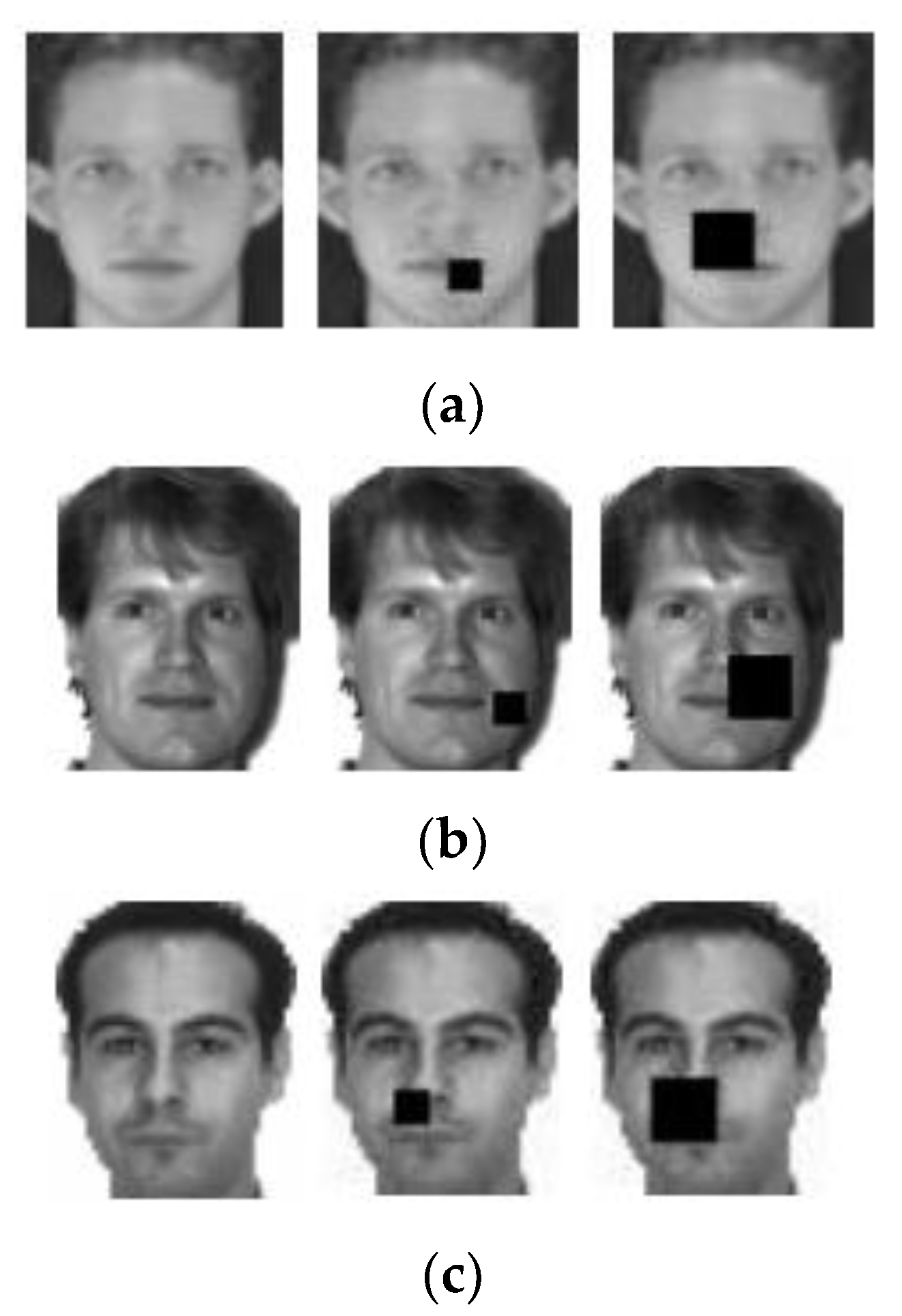
4.4. The FERET Face Database
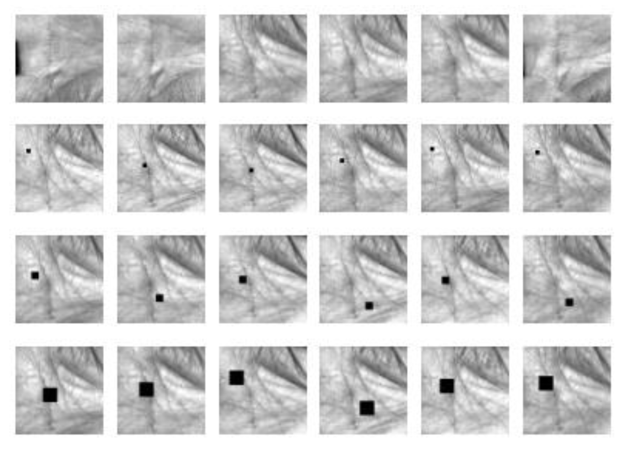
4.5. The PolyU Palmprint Verification Experiment
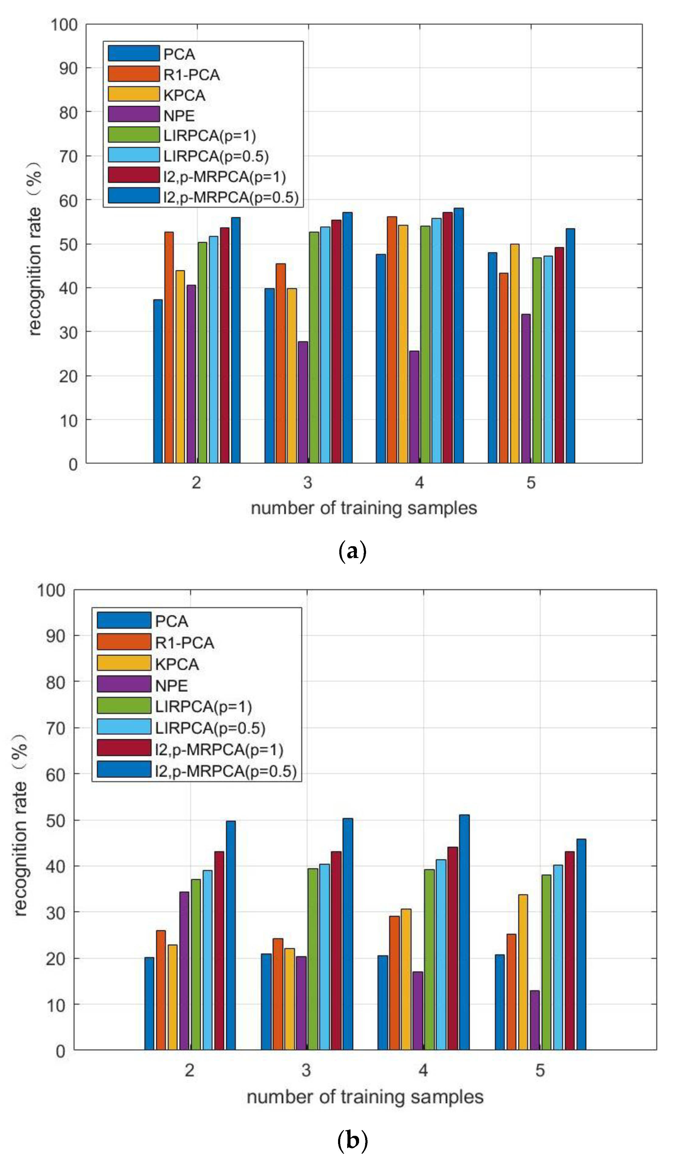
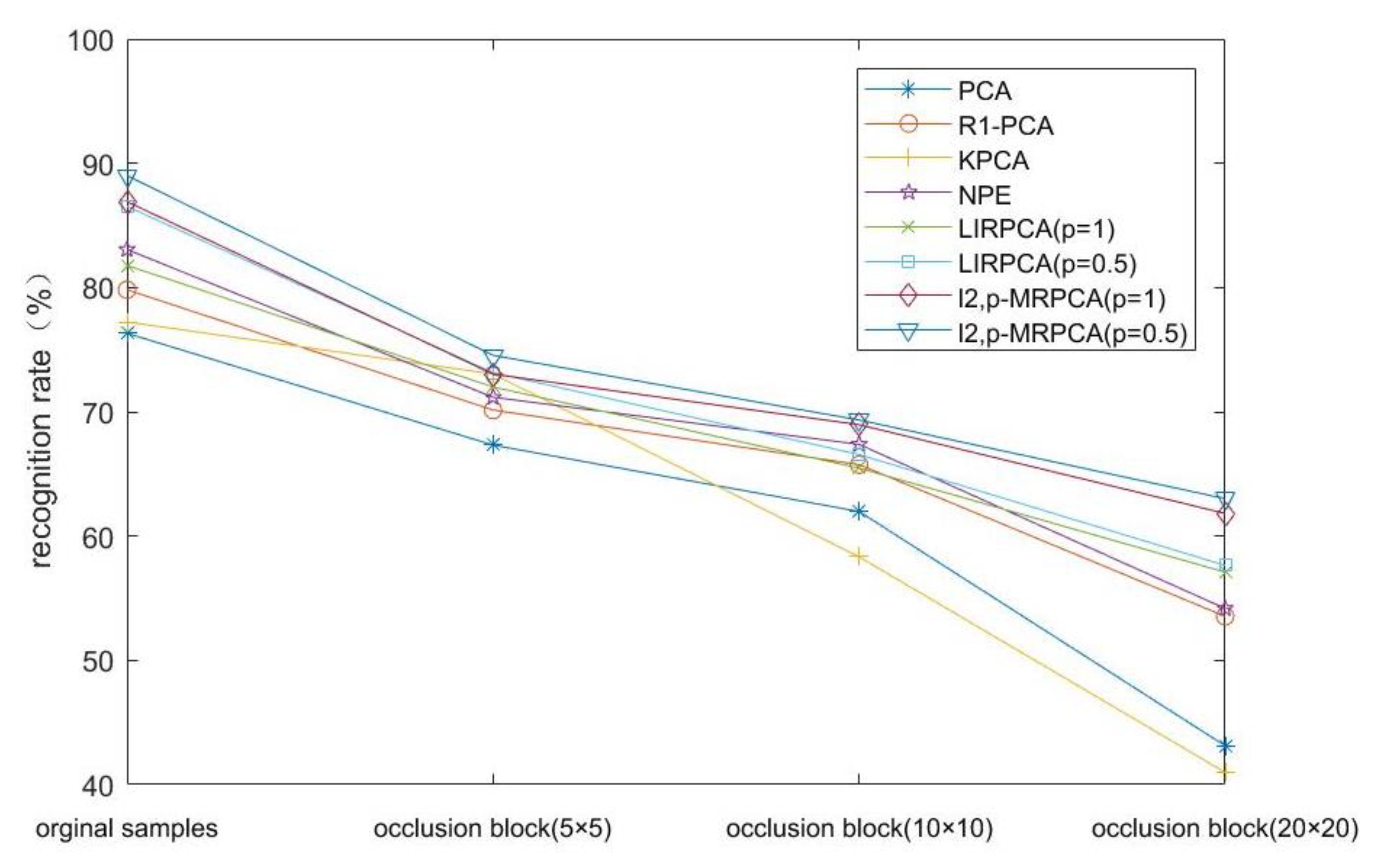
4.6. Result Analysis
- 1.
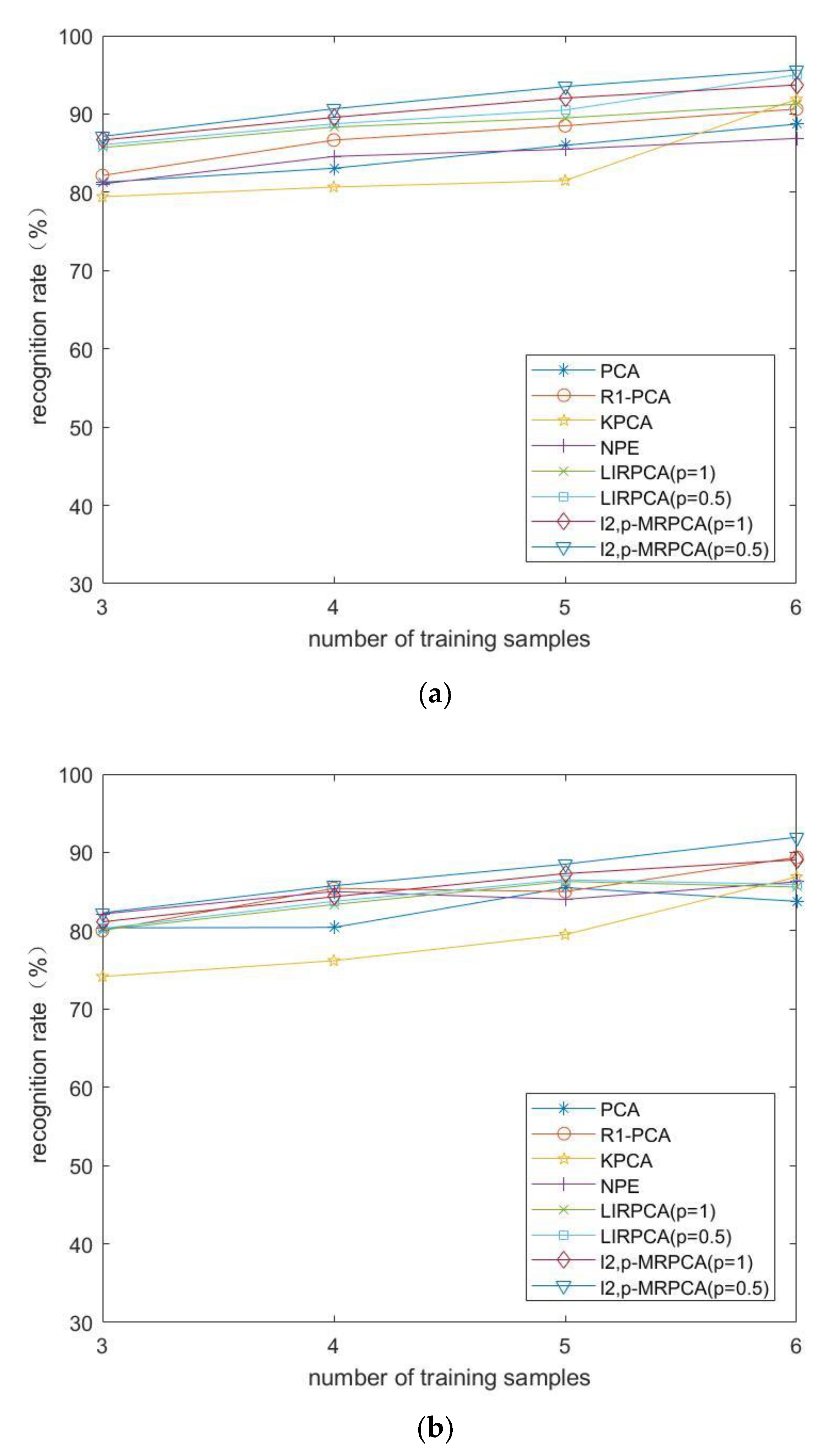
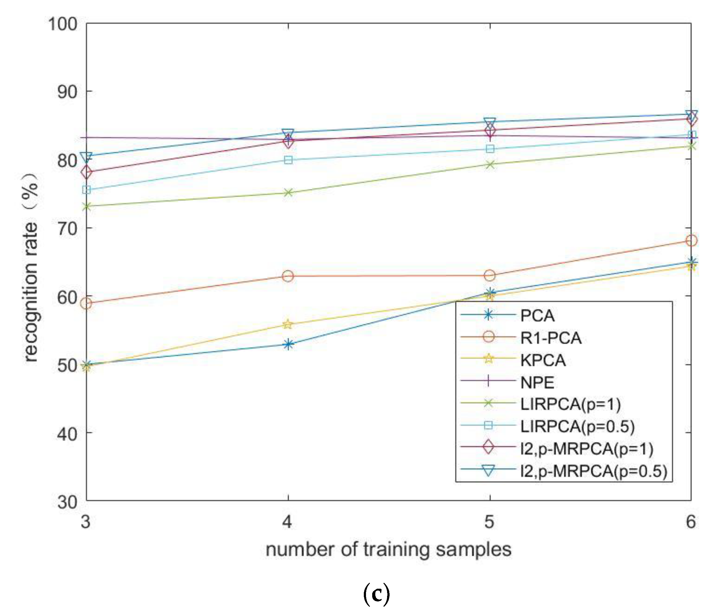
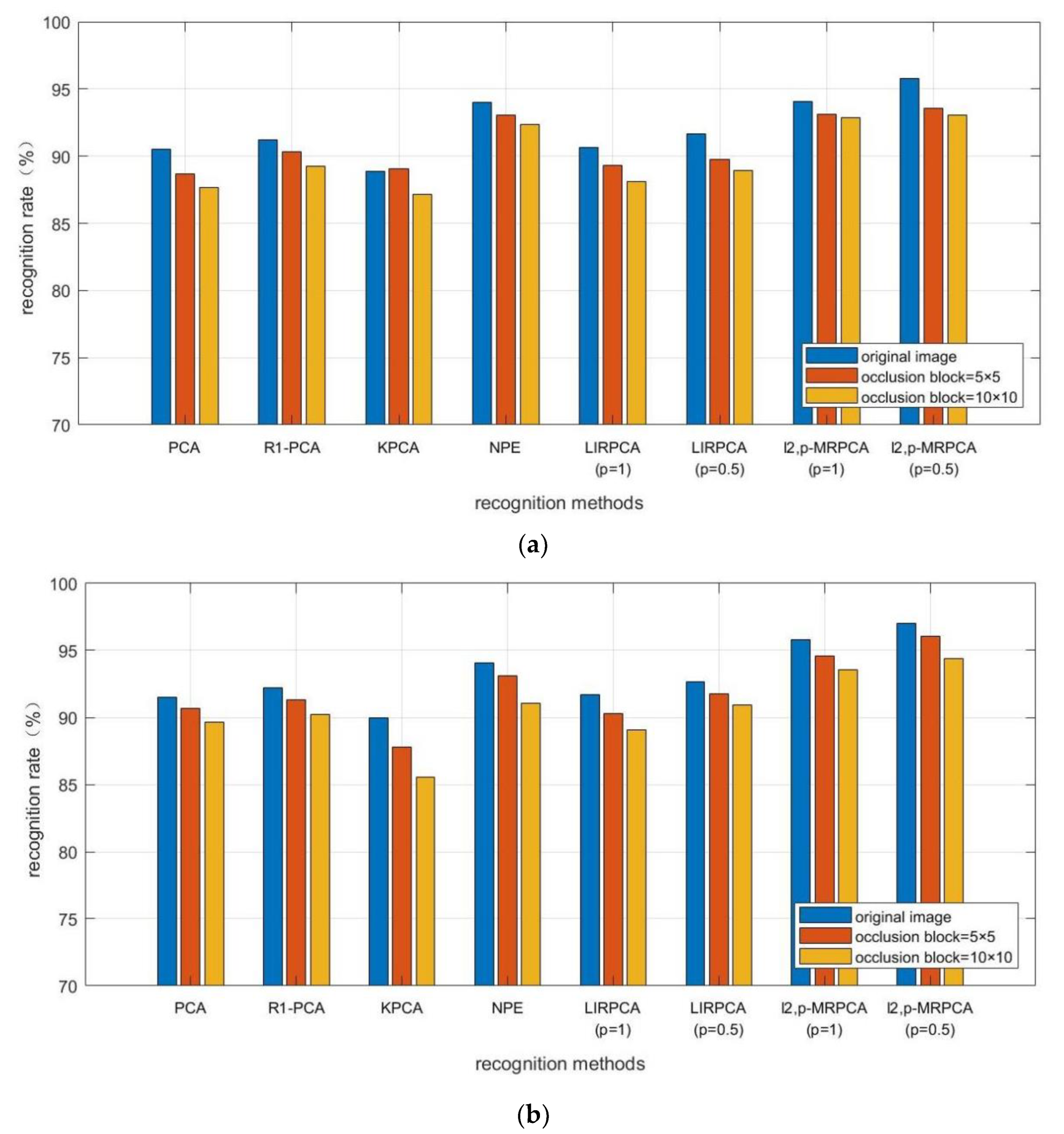
- From the experimental results, -PCA, as an improved algorithm of PCA algorithm, has a high recognition rate both in the original image database and in the occluded database.
- 2.
- When the experimental data is occluded, NPE, as a manifold learning method, most of the recognition rates are higher than PCA, indicating that the algorithm is less affected by occlusion. When the image is occluded, the recognition effect is better.
- 3.
- Compared to LIRPCA, -MRPCA introduces manifold learning method, so the recognition rate is more significant. In addition, it takes into account the advantages of manifold regularization when the image is occluded, so the recognition effect is better. As the clarity of each database in the experiment is different, the recognition rate made by different databases is relatively different.
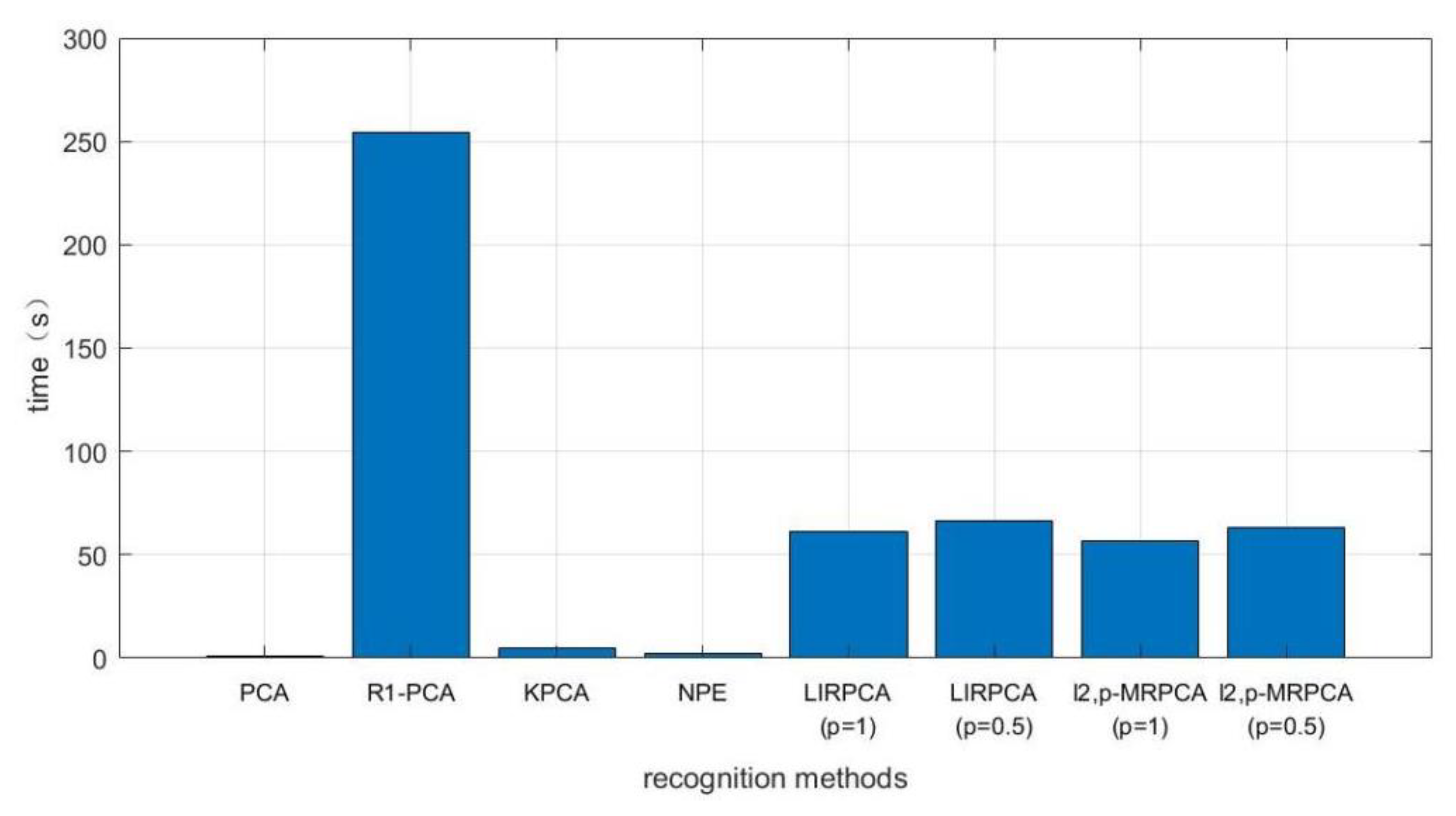
- 4.
- The training time on -MRPCA is longer than PCA, KPCA and NPE, and is shorter than -PCA and LIRPCA. Considering the recognition rate, robustness, and algorithm time of the algorithm, the training time on -MRPCA is acceptable.
- 5.
- The parameter also has a certain impact on the recognition effect. Whether it is LIRPCA or -MRPCA, the recognition efficiency is slightly higher when than when .
5. Conclusions
- 1.
- Optimize the formula of -MRPCA;
- 2.
- the equation of the optimal matrix is obtained by using KKT condition;
- 3.
- and according to the algorithm proposed in this paper, the convergence of the objective function is obtained, and the optimal projection matrix is obtained.
Author Contributions
Funding
Institutional Review Board Statement
Informed Consent Statement
Data Availability Statement
Conflicts of Interest
References
- Wu, X.T.; Yan, Q.D. Analysis and Research on data dimensionality reduction method. Comput. Appl. Res. 2009, 26, 2832–2835. [Google Scholar]
- Yu, X.X.; Zhou, N. Research on dimensionality reduction method of high-dimensional data. Inf. Sci. 2007, 25, 1248–1251. [Google Scholar]
- Wan, M.H.; Lai, Z.H.; Yang, G.W. Local graph embedding based on maximum margin criterion via fuzzy set. Fuzzy Sets Syst. 2017, 2017, 120–131. [Google Scholar] [CrossRef]
- Yang, J.; Zhang, D.D.; Yang, J.Y. Constructing PCA Baseline Algorithms to Reevaluate ICA-Based Face-Recognition Performance. IEEE Trans Multimed. 2007, 37, 1015–1021. [Google Scholar]
- Zuo, W.; Zhang, D.; Yang, J.; Wang, K. BDPCA plus LDA:a novel fast feature extraction technique for face recognition. IEEE Trans. Syst. Man Cybern. B Cybern. 2006, 36, 946–953. [Google Scholar]
- Kim, Y.G.; Song, Y.J.; Chang, U.D.; Kim, D.W.; Yun, T.S.; Ahn, J.H. Face recognition using a fusion method based on bidirectional 2DPCA. Appl. Math. Comput. 2008, 205, 601–607. [Google Scholar] [CrossRef]
- Yang, J.; Zhang, D.; Frangi, A.F.; Yang, J.Y. Two dimensional PCA: A new approach to appearance-based face representation and recognition. IEEE Trans. Pattern Anal. Mach. Intell. 2004, 26, 131–137. [Google Scholar] [CrossRef]
- Yang, J.; Zhang, D.; Yong, X.; Yang, J.Y. Two dimensional discriminant transform for face recognition. Pattern Recognit. 2005, 38, 1125–1129. [Google Scholar] [CrossRef]
- Wang, J.; Barreto, A.; Wang, L.; Chen, Y.; Rishe, N.; Andrian, J.; Adjouadi, M. Multilinear principal component analysis for face recognition with fewer features. Neurocomputing 2010, 73, 1550–1555. [Google Scholar] [CrossRef]
- Wan, M.; Yao, Y.; Zhan, T.; Yang, G. Supervised Low-Rank Embedded Regression (SLRER) for Robust Subspace Learning. IEEE Trans. Circuits Syst. Video Technol. 2022, 32, 1917–1927. [Google Scholar] [CrossRef]
- Wright, J.; Ganesh, A.; Rao, S.; Peng, Y.; Ma, Y. Robust Principal Component Analysis: Exact Recovery of Corrupted Low-Rank Matrice. Adv. Neural Inf. Process. Syst. 2009, 22, 2080–2088. [Google Scholar]
- Wan, M.; Chen, X.; Zhao, C.; Zhan, T.; Yang, G. A new weakly supervised discrete discriminant hashing for robust data representation. Inf. Sci. 2022, 611, 335–348. [Google Scholar] [CrossRef]
- Ke, Q.F.; Kanade, T. Robust L1 norm factorization in the presence of outliers and missing data by alternative convex programming. In Proceedings of the IEEE Computer Society Conference on Computer Vision & Pattern Recognition, San Diego, CA, USA, 20–25 June 2005; Volume 1, pp. 739–746. [Google Scholar]
- He, R.; Hu, B.G.; Zheng, W.S.; Kong, X.W. Robust Principal Component Analysis Based on Maximum Correntropy Criterion. IEEE Trans. Image Process. 2011, 20, 1485–1494. [Google Scholar]
- Kwak, N. Principal Component Analysis Based on L1-Norm Maximization. IEEE Trans. Pattern Anal. Mach. Intell. 2008, 30, 1672–1680. [Google Scholar] [CrossRef] [PubMed]
- Kwak, N. Principal Component Analysis by L-p-Norm Maximization. IEEE Trans. Cybern. 2014, 44, 594–609. [Google Scholar] [CrossRef] [PubMed]
- Ye, Q.; Fu, L.; Zhang, Z.; Zhao, H.; Naiem, M. Lp- and Ls-Norm Distance Based Robust Linear Discriminant Analysis. Neural Netw. 2018, 105, 393–404. [Google Scholar] [CrossRef]
- Ding, C.; Zhou, D.; He, X.; Zha, H. R1-PCA:Rotational invariant L1-norm principal component analysis for robust subspace factorization. In Proceedings of the 23rd International Conference on Machine Learning, ACM, New York, NY, USA, 25–29 June 2006; pp. 281–288. [Google Scholar]
- Wang, Q.; Gao, Q.; Gao, X.; Nie, F. L2,p-norm based PCA for image recognition. IEEE Trans. Image Process. 2008, 27, 1336–1346. [Google Scholar] [CrossRef]
- Bi, P.; Du, X. Application of Locally Invariant Robust PCA for Underwater Image Recognition. IEEE Access 2021, 9, 29470–29481. [Google Scholar] [CrossRef]
- Xu, J.; Bi, P.; Du, X.; Li, J.; Chen, D. Generalized Robust PCA: A New Distance Metric Method for Underwater Target Recognition. IEEE Access 2019, 7, 51952–51964. [Google Scholar] [CrossRef]
- Wan, M.; Chen, X.; Zhan, T.; Xu, C.; Yang, G.; Zhou, H. Sparse Fuzzy Two-Dimensional Discriminant Local Preserving Projection (SF2DDLPP) for Robust Image Feature Extraction. Inf. Sci. 2021, 563, 1–15. [Google Scholar] [CrossRef]
- Tasoulis, S.; Pavlidis, N.G.; Roos, T. Nonlinear Dimensionality Reduction for Clustering. Pattern Recognit. 2020, 107, 107508. [Google Scholar] [CrossRef]
- Luo, W.Q. Face recognition based on Laplacian Eigenmaps. In Proceedings of the International Conference on Computer Science and Service System, Nanjing, China, 27–29 June 2011; pp. 27–29. [Google Scholar]
- Roweis, S.; Saul, L. Nonlinear Dimensionality Reduction by Locally Linear Embedding. Science 2000, 290, 2323–2326. [Google Scholar] [CrossRef] [PubMed]
- Hu, K.L.; Yuan, J.Q. Statistical monitoring of fed-batch process using dynamic multiway neighborhood preserving embedding. Chemom. Intell. Lab. Syst. 2008, 90, 195–203. [Google Scholar] [CrossRef]
- Song, B.; Ma, Y.; Shi, H. Multimode process monitoring using improved dynamic neighborhood preserving embedding. Chemom. Intell. Lab. Syst. 2014, 135, 17–30. [Google Scholar] [CrossRef]
- Wan, M.; Chen, X.; Zhan, T.; Yang, G.; Tan, H.; Zheng, H. Low-rank 2D Local Discriminant Graph Embedding for Robust Image Feature Extraction. Pattern Recognit. 2023, 133, 109034. [Google Scholar] [CrossRef]
- Chen, X.; Wan, M.; Zheng, H.; Xu, C.; Sun, C.; Fan, Z. A New Bilinear Supervised Neighborhood Discrete Discriminant Hashing. Mathematics 2022, 10, 2110. [Google Scholar] [CrossRef]
- Li, W.H.; Gong, W.G.; Cheng, W.M. Method based on wavelet multiresolution analysis and KPCA for face recognition. Comput. Appl. 2005, 25, 2339–2341. [Google Scholar]
- De, F.; Torre, L.; Black, M.J. A Framework for Robust Subspace Learning. Int. J. Comput. Vis. 2003, 54, 117–142. [Google Scholar]


| TN | 3 | |||
|---|---|---|---|---|
| Occlusion Block Size | None | 5 × 5 | 10 × 10 | 20 × 20 |
| PCA/% | 76.32 (0.53) | 67.32 (0.51) | 61.98 (0.49) | 43.12 (0.22) |
| R1-PCA/% | 79.82 (0.42) | 70.14 (0.44) | 65.75 (0.53) | 53.54 (0.35) |
| KPCA/% | 77.23 (0.12) | 73.04 (0.50) | 58.33 (0.49) | 40.98 (0.16) |
| NPE/% | 83.06 (0.42) | 71.17 (0.44) | 67.38 (0.47) | 54.17 (0.54) |
| LIRPCA (p = 1)/% | 81.78 (0.27) | 72.00 (0.33) | 65.47 (0.35) | 57.10 (0.41) |
| LIRPCA (p = 0.5)/% | 86.53 (0.32) | 73.15 (0.35) | 66.56 (0.31) | 57.64 (0.29) |
| -MRPCA (p = 1)/% | 86.91 (0.30) | 73.03 (0.38) | 68.96 (0.32) | 61.82 (0.07) |
| -MRPCA (p = 0.5)/% | 89.01 (0.33) | 74.54 (0.36) | 69.34 (0.35) | 63.01 (0.43) |
Publisher’s Note: MDPI stays neutral with regard to jurisdictional claims in published maps and institutional affiliations. |
© 2022 by the authors. Licensee MDPI, Basel, Switzerland. This article is an open access article distributed under the terms and conditions of the Creative Commons Attribution (CC BY) license (https://creativecommons.org/licenses/by/4.0/).
Share and Cite
Wan, M.; Wang, X.; Tan, H.; Yang, G. Manifold Regularized Principal Component Analysis Method Using L2,p-Norm. Mathematics 2022, 10, 4603. https://doi.org/10.3390/math10234603
Wan M, Wang X, Tan H, Yang G. Manifold Regularized Principal Component Analysis Method Using L2,p-Norm. Mathematics. 2022; 10(23):4603. https://doi.org/10.3390/math10234603
Chicago/Turabian StyleWan, Minghua, Xichen Wang, Hai Tan, and Guowei Yang. 2022. "Manifold Regularized Principal Component Analysis Method Using L2,p-Norm" Mathematics 10, no. 23: 4603. https://doi.org/10.3390/math10234603
APA StyleWan, M., Wang, X., Tan, H., & Yang, G. (2022). Manifold Regularized Principal Component Analysis Method Using L2,p-Norm. Mathematics, 10(23), 4603. https://doi.org/10.3390/math10234603