Methodology of Plasma Shape Reachability Area Estimation in D-Shaped Tokamaks

Abstract

This paper suggests and develops a new methodology of estimation for a multivariable reachability region of a plasma separatrix shape on the divertor phase of a plasma discharge in D-shaped tokamaks. The methodology is applied to a spherical Globus-M/M2 tokamak, including the estimation of a controllability region of a vertical unstable plasma position on the basis of the experimental data. An assessment of the controllability region and the reachability region of the plasma is important for the design of tokamak poloidal field coils and the synthesis of a plasma magnetic control system. When designing a D-shaped tokamak, it is necessary to avoid the small controllability region of the vertically unstable plasma, because such cases occur in practice at a restricted voltage on a horizon field coil. To make the estimations mentioned above robust, PID-controllers for vertical and horizontal plasma position control were designed using the Quantitative Feedback Theory approach, which stabilizes the system and provides satisfactory control indexes (stability margins, setting time, overshoot) during plasma discharges. The controllers were tested on a series of plasma models and nonlinear models of current inverters in auto-oscillation mode as actuators for plasma position control. The estimations were made on these models, taking into account limitations on control actions, i.e., voltages on poloidal field coils. This research is the first step in the design of the plasma shape feedback control system for the operation of the Globus-M2 spherical tokamak. The developed methodology may be used in the design of poloidal field coil systems in tokamak projects in order to avoid weak achievability and controllability regions in magnetic plasma control. It was found that there is a strong cross-influence from the PF-coils currents and the CC current on the plasma shape; hence, these coils should be used to control the plasma shape simultaneously.

1. Introduction

1.1. Background

Tokamaks (toroidal vessels with magnetic coils) are the most promising devices for solving the controlled fusion problem [1]. In particular, tokamaks are classified by an aspect ratio, A (ratio of a tokamak major radius to a minor radius). One has to differentiate conventional ($A\approx 3÷4$) and spherical ($A\approx 1.4÷1.7$) tokamaks (see the surveys in [2,3,4,5]). Spherical tokamaks, in comparison with conventional tokamaks, have a number of advantages: better plasma confinement, higher values of safety factor $q$ on a plasma boundary, higher values of magnetic and electric fields, etc. These features make the creation and operation of fusion power plants on the basis of spherical tokamaks much cheaper than power plants based on conventional tokamaks [6,7].

The development of the first DEMO (DEMOnstration Power Plant) as a fusion power plant was accompanied by an increase in the size of the devices used to achieve the Lawson criteria [8], correspondingly increasing their cost and the time required to build them [6,7]. According to expert estimations, the first commercial fusion power plant based on tokamaks with a relatively large aspect ratio should be built by about 2075 [6]. However, there is an alternative approach in which the fusion plant is built up using several modules, with each module being a spherical tokamak. The construction of such a power plant is much cheaper compared with using DEMO on the conventional tokamak and can be implemented in about fifteen years [6]. Due to plasma properties, it is possible to create a spherical tokamak module with a major radius of ~1.5–1.7 m. In contrast to these plants, the conventional DEMO major radius is about 9 m. According to modern estimates, a module fusion power plant is able to provide highly competitive electricity for less than 0.06 $/kWh. In this regard, the work on the development, creation, and operation of spherical tokamaks is important and promising [6,7]. Advanced plasma magnetic control systems are able to provide the reliable operation of tokamaks and fusion power plants on the basis of tokamaks. Because of this, developments in plasma magnetic control systems for tokamaks are of great importance.

1.2. Motivation and Novelty

This paper is devoted to plasma magnetic control systems, the controllability region of the plasma unstable vertical position, and the reachability areas of a separatrix of the divertor phases of discharges in the spherical Globus-M/M2 tokamak (Ioffe Institute, Saint Petersburg, Russia) [9,10]. Usually, this topic is not investigated in detail for tokamaks and their poloidal systems in projects and in experiments, despite plasma magnetic control systems being developed and applied in practice [2,3,4,5]. However, such inaction in this matter sometimes leads to faults in tokamak plasma poloidal systems, which create serious difficulties for plasma control. For instance, in [11], a very narrow controllability region in the plasma vertical direction of ITER was discovered. It forced the ITER project team to put additional horizon field coils (HFC) inside the vacuum vessel (VV) to significantly increase this region [11]. In the tokamak T-15MD project (Kurchatov Institute, Moscow, Russia), the HFC took place near poloidal field (PF) coils, which screened the HFC and made the whole plasma vertical position control system internally unstable. This situation forced the tokamak designers to place this coil between the VV and the toroidal field coil, and that provided an acceptable controllability region for plasma movement in the vertical direction [12]. In [13], the optimal location of HFC in the IGNITOR tokamak was found for the first time with optimization criterion in the form of the size of the vertical controllability region inside the toroidal field coil, near the VV.

This situation motivated us to suggest and develop a methodology of estimation for a multivariable reachability region in a plasma separatrix shape on the divertor phase of plasma discharges in D-shaped tokamaks. The divertor phase is a key part of plasma discharge when the plasma is held in a vacuum vessel only by magnetic fields and does not touch the vessel walls. Depending on various discharge parameters, the start time, duration, and end time of the divertor phase may be different.

In the case of the operating spherical Globus-M2 tokamak, studying the controllability region in the vertical direction made it possible to estimate the stability margin in the presence of the restriction on the HFC voltage. A new study of the upper and lower boundaries of the reachability area for the plasma shape of the Globus-M2 tokamak will provide a chance to estimate the margins of the plasma separatrix location, when the plasma shape feedback control system will be applied in the presence of restrictions on PF-coil voltages. The basic preparations that form the basis of simulations for such physical experiments with a feedback plasma shape control system were performed in [14,15,16].

1.3. State-of-the-Art and Beyond-the-State-of-the-Art

Numerical and analytical approaches to the controllability areas in tokamaks were considered in [11,12,13,17,18]. These methods form the basis of controllability area estimates for the Globus-M/M2. In this work, specific methods for estimating the reachability region were developed for linear dynamic systems in a steady-state regime in general and for plasma shape control in the tokamak in particular. In [19], a numerical analysis of the sensitivity of plasma shape gaps to poloidal field coil currents of the FAST tokamak was performed, which is the first step of the plasma position multivariable reachability region estimation proposed in this article for the Globus-M2 tokamak

1.4. Hypothesis

With the help of plasma models of the Globus-M/M2 tokamaks, it is possible to estimate and compare the controllability area of the unstable vertical plasma position and the reachability area of the plasma shape. To do this, robust PID-controllers for plasma position control are needed. The tuning of PID-controllers is performed using the well-known Quantitative Feedback Theory (QFT) approach [20]. The vertical controllability region is estimated using numerical simulations of plasma discharges with different initial displacements and analytically by diagonalizing the A-matrix of the state–space model of the plasma without a vertical position PID-controller. The reachability region of the plasma shape is estimated by using the matrix relation between the inputs and outputs of the linear model in the steady-state regime on the basis of the developed methodology.

1.5. Paper Organization

The paper is organized in the following way. Section 2 describes the tokamak, models, and goals of this work. Section 3 presents the tuning and numerical proving of plasma position PID-controllers. In Section 4, the estimation of the controllability region of the vertical plasma position was made using an analytical approach with the help of numerical simulations. Section 5 presents a new estimation of the reachability region of the plasma shape by means of the new methodology. The Conclusion summarizes the basic results of the paper.

2. Problem Description

2.1. Globus-M2 Tokamak

The operating spherical Globus-M2 tokamak is shown in Figure 1. The vertical cross-section of the Globus-M/M2 tokamak, with the locations of PF coils and VV elements, is presented in Figure 2a. The basic parameters of this device are as follows: major radius, R = 0.36 m; minor radius, a = 0.24 m; aspect ratio, R/a = 1.5; toroidal magnetic field, B_{t max} = 1 T; plasma current, 0.5 MA; impulse duration, less than 0.7 s [9,10].

2.2. Plasma Control System Structure

There are eight PF-coils in the Globus-M/M2 tokamak. They are used for plasma control. The HFC controls the vertical plasma position; the vertical field coil (VFC) controls the horizontal plasma position. Currents in these coils are supplied by thyristor current inverters that operate in self-oscillation mode [15]. These devices have a self-oscillation frequency of up to 3 kHz, which is necessary for high-performance plasma position control. The central solenoid (CS), correcting coil (CC), and four poloidal field (PF) coils (PF1, PF2top, PF2bottom and PF3) can be used for plasma shape control (Figure 2b,c). The plasma shape in this paper is determined by four gaps between the plasma separatrix and the first wall of the VV and the positions of two intersection points of the separatrix and the first wall (Figure 2b,c).

2.3. Linear Plasma Model

The linear plasma model was obtained from Kirchhoff’s law equations for the PF coils, VV elements, and plasma column, as well as Newton’s law of motion for the plasma vertical and horizontal positions [16]:

$$\{\begin{array}{c}\dot{\Psi }[J(t),R,Z]+R_{c}I=U, \\ m\ddot{Z}=F_Z[J(t),I,R,Z], \\ m\ddot{R}=F_R[J(t),I,R,Z].\end{array}$$

(1)

where $I={\left[\begin{array}{ccc}{I}_c^T& I_v^T& I_p\end{array}\right]}^T$ is the vector- column of currents in the PF coils, VV, and plasma; $\Psi$ is the vector-column of magnetic fluxes through areas encircled by the currents; $J(t)$ is the plasma current density distribution; $R_c$ is the diagonal matrix of PF, VV, and plasma electrical resistances; $U$ is the vector-column of voltages applied to the circuits; m is the plasma mass; $Z$ and $R$ are plasma coordinates; $F_R$ and $F_Z$ are horizontal and vertical forces acting on the plasma.

Changes in the plasma shape are described by projections of the displacements of six points P1–P6 on the plasma separatrix in the corresponding directions indicated by arrows in Figure 2b,c. The plasma shape changes with plasma movement and changes currents in the system:

$$P=P[J(t),I,R,Z],$$

(2)

where $P={\left[\begin{array}{cccccc}P1& P2& P3& P4& P5& P6\end{array}\right]}^T$.

In the equilibrium the effect of forces $F_R$ and $F_Z$ on the plasma is zero, but the vertical plasma displacements increase the vertical force, $\frac{\partial F_Z}{\partial Z}>0$, causing instability in the controlled plant. The horizontal plasma position is stable; thus, $\frac{\partial F_R}{\partial R}<0$, allowing us to neglect the small plasma mass in the horizontal motion equation.

Model Equations (1) and (2), used for small deviations from the plasma equilibrium, are written as follows:

$$\begin{array}{c}M[J(t),R,Z]\delta \dot{I}+RI+\frac{\partial }{\partial R}\Psi [J(t),R,Z]\delta R+\frac{\partial }{\partial Z}\Psi [J(t),R,Z]\delta Z=\delta U,\\ m\ddot{Z}=\frac{\partial }{\partial I}{F}_Z[J(t),I,R,Z]\delta I+\frac{\partial }{\partial R}{F}_Z[J(t),I,R,Z]\delta R+\frac{\partial }{\partial Z}{F}_Z[J(t),I,R,Z]\delta Z,\\ 0=\frac{\partial }{\partial I}{F}_R[J(t),I,R,Z]\delta I+\frac{\partial }{\partial R}{F}_R[J(t),I,R,Z]\delta R+\frac{\partial }{\partial Z}{F}_R[J(t),I,R,Z]\delta Z,\\ \delta P=\frac{\partial }{\partial I}P[J(t),I,R,Z]\delta I+\frac{\partial }{\partial R}P[J(t),I,R,Z]\delta R+\frac{\partial }{\partial Z}P[J(t),I,R,Z]\delta Z.\end{array}$$

(3)

With the introduction of the state vector, $x={\left[\begin{array}{ccc}\delta I^T& \delta \dot{Z}& \delta Z\end{array}\right]}^T,$ the input vector, $u=\delta U,$ the output vector $y={\left[\begin{array}{cccc}\delta Z& \delta R& \delta I_c^T& \delta P^T\end{array}\right]}^T,$ and the linear transformation, the model Equation (3) is written in the standard form of the state–space model:

$$\begin{array}{l}\dot{x}=Ax+Bu, \\ y=Cx.\end{array}$$

(4)

In this work, one model for the Globus-M plasma and five models for the Globus-M2 plasma are used (each model corresponds to different tokamak shots). The plasma current density, $J(t)$; plasma coordinates, $R, Z$; and currents, $I$, in the system are identified from experimental data via plasma equilibrium reconstruction code FCDI [16]. For each shot, a set of linear time-invariant (LTI) models corresponding to plasma equilibria at different time points of the shots were constructed. Each plasma model (4) has 26 states for Globus-M2 and 24 states for Globus-M, 8 inputs, and 16 outputs: $x\in {ℝ}^{26}, u\in {ℝ}^8, y \in {ℝ}^{16}, A\in {ℝ}^{26\times 26}, B\in {ℝ}^{26\times 8}, C\in {ℝ}^{16\times 26}$. The inputs are voltages on the PF-coils; the outputs are the plasma position, the currents in the PF-coils, and the plasma shape. The parameters of the plasma change during plasma discharge. Because of this, instead of using one model (4), each set of plasma models was interpolated into a time-dependent model:

$$\begin{array}{l} \dot{x}=A(t)x+B(t)u, \\ y=C(t)x,\\ x\in {ℝ}^{26}, u\in {ℝ}^8, y \in {ℝ}^{16}, A\in {ℝ}^{26\times 26}, B\in {ℝ}^{26\times 8}, C\in {ℝ}^{16\times 26}.\end{array}$$

(5)

2.4. Problem Statements

Problems to be solved:

• Tuning of the robust PID-controllers of the vertical and horizontal plasma positions.

The problem of PID-controller tuning is finding controller parameters so that an A matrix of the state–space equation of a closed loop system in continuous time becomes stable (the real part of all eigenvalues of A should be negative): $\forall i real({\lambda }_i(A))<0$. The setting time is about 10 ms, and the overshot is less than 20%.

• Estimation of the size of the unstable vertical plasma position controllability region.

The controllability region of the vertical plasma position means that the control system is able to transfer any vertical plasma position in that region to any state inside that region in a finite time interval; in doing so, a control action is kept within the allowable limits (the voltage on the HFC is less than 900 V), and other states at $t=0$ are equal to zero:

$$\begin{array}{l}v=\max \left|Z_0\right|:\\ \forall \tilde{z}\in [-v,+v]: \exists u(t): \max |u(t)|\le u_{\max }, Z_0=z(0)=y_1(0): z(t)\to \tilde{z}.\end{array}$$

(6)

• Estimation of the plasma shape reachability area

Estimation of the reachability area of the plasma shape is divided into two parts: the upper and lower estimations. This separation is necessary because the reachability area is multivariable: eight inputs and six outputs are involved, and each input influences each output. Two kinds of estimation provide more information about the reachability area.

The upper estimation of each gap is the maximum value of this gap, which is independent of other gaps (the values of other gaps can be any.

The lower estimation is the maximum value within which all gaps can change simultaneously.

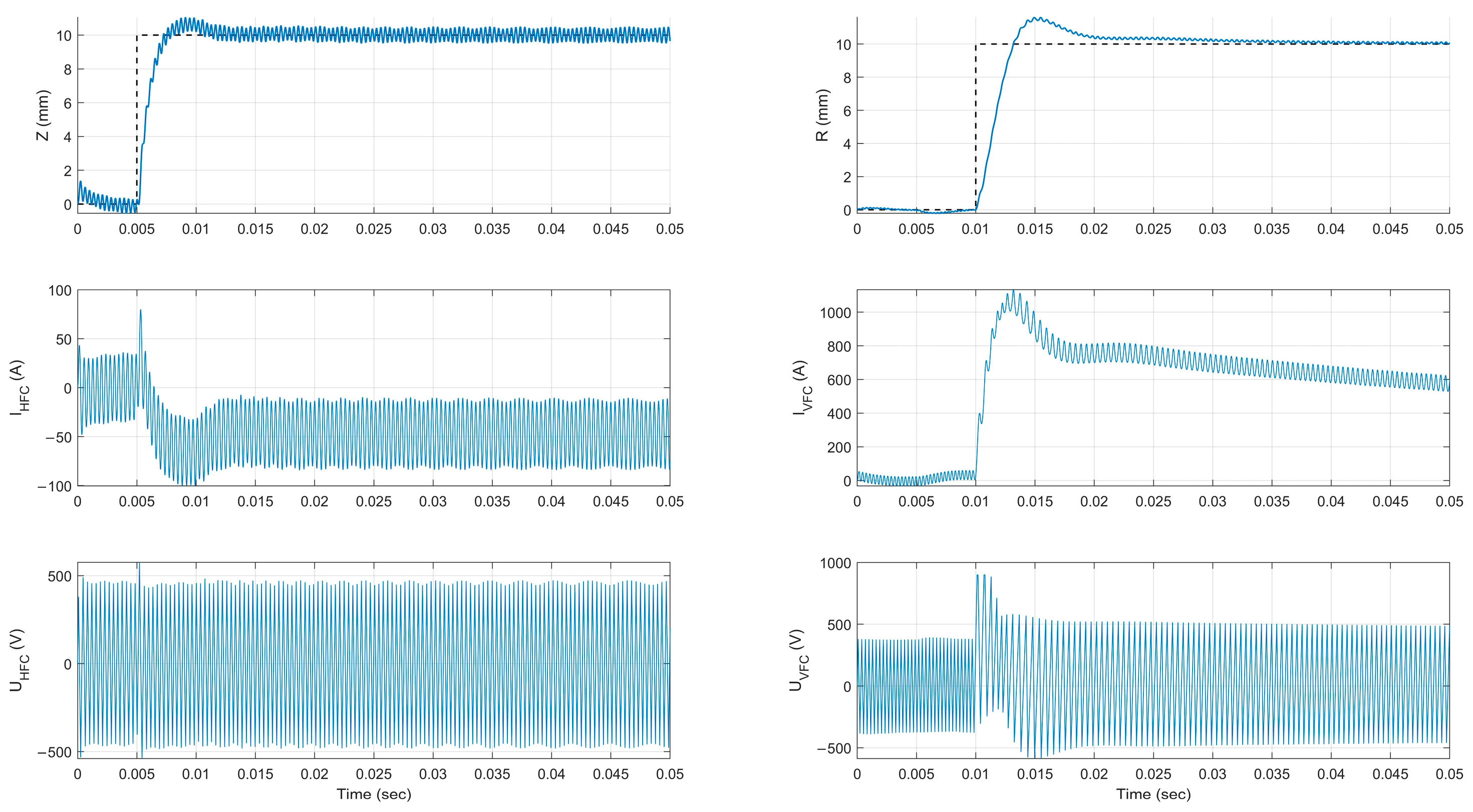
3. Plasma Position PID-Controllers Tuning

Plasma position controllers are critically important for the operation of the plasma magnetic control system as a whole. For plasma position control, it is necessary to rapidly change the currents in the HFC and VFC. There are two thyristor current inverters (Figure 3) in the plasma position control loops for this goal [15]. In this paper, the proportional gain is used as a current inverter model for PID-controller tuning, and a nonlinear model is used for testing. The first reason to design robust controllers is a very rough approximation of the current inverter. The second reason is the uncertainties and time-variance in the plasma model.

The QFT approach was chosen for PID-controller tuning (Figure 4) [20]. This theory allows us to tune robust controllers in the frequency domain with the help of a Nichols diagram, taking into account uncertainness in the controlled plant model. The Nichols diagram displays $20lo{g}_{10}\left(|G(s)|\right)$ versus $arg\left(G(s)\right)$, where $G(s)$ is the transfer function of the open-loop system. QFT allows us to use a set of models in format of Equation (4) instead of a parameter-varying model (5). The distance from point $\left(-180°, 0 \mathrm{dB}\right)$ to the intersection with the X-axis in the Nichols diagram is a phase margin; the distance to the intersection with the Y-axis in the Nichols diagram is an amplitude margin (Figure 5) [21,22].

A piecewise cubic Hermite interpolation polynomial (PCHIP) approach [23] in the MATLAB environment was used to obtain the values of the phase and amplitude margins between points corresponding to the linear models (Figure 5). The advantages of the PCHIP approach are the absence of overshoots and fewer oscillations in comparison with other interpolation methods [23]. If there are n points ($\left\{\left(x_1, f_1\right), \dots , \left(x_n, f_n\right)\right\}$) then on the ith subinterval ($[x_i, x_{i+1}]$) the PCHIP creates a cubic polynomial

$$f_i(x)=a{(x-x_i)}^3+b{(x-x_i)}^2+c(x-x_i)+y_i,$$

(7)

with the following properties:

$$\begin{array}{c}{f}_i(x_{i+1})=y_{i+1},\\ \frac{d{f}_i(x_{i+1})}{dx}=\frac{d{f}_{i+1}(x_{i+1})}{dx},\end{array}\forall i=1, \dots , n-2$$

(8)

Thus, we find that the piecewise function is continuous and continuously differentiable.

A set of plasma models corresponding to Globus-M2 tokamak shot #37239 [10] was used to tune the PID controllers. Tuning was performed using the MATLAB QFT Control Toolbox [24], which provided vertical and horizontal plasma position PID-controllers:

$$\begin{array}{l}{\mathrm{PID}}_{\mathrm{Z}}\left(\mathrm{s}\right)=43.8+\frac{7790}{\mathrm{s}}+0.0561\frac{\mathrm{13,300}}{1+\mathrm{13,300}/\mathrm{s}}, \\ {\mathrm{PID}}_{\mathrm{R}}\left(\mathrm{s}\right)=2+\frac{2·{10}^4}{\mathrm{s}}+10\frac{10}{1+10/\mathrm{s}}.\end{array}$$

(9)

The minimal amplitude and phase margins of the systems with different models are 8.2 dB and 49.3° for the vertical positions and 51.7 dB and 65.7° for the horizontal positions (Figure 5). The setting time is about 10 ms, and the overshot is about 20% in testing the systems using step-functions (Figure 6).

For overshot, decreasing the pre-filter with the transfer function, $PF(s)=\frac{{10}^3}{s+{10}^3}$ (Figure 3), was involved in the vertical position control loop. Its influence is shown in Figure 7a. The robust properties of the obtained PID-controllers are presented in Figure 7b. This involved a set of step responses for the systems with plasma models corresponding to different moments of the different plasma shots. Eighteen plasma models corresponding to shots #37239, #37255, #37257, #37702, and #37712 of the spherical Globus-M2 tokamak were used; vertical and horizontal plasma position control systems were modeled.

4. Estimation of the Controllability Region of the Unstable Vertical Plasma Position

4.1. Statement of the Estimation Problem

The controllability region of the unstable vertical plasma position (6) is an important parameter in a D-shaped tokamak. The plasma beyond the controllability area is uncontrollable and unstable. This causes high-temperature plasma ejection onto the VV wall, which can lead to its destruction. The problem of the small controllability region was detected during the design of the ITER [11] and T-15MD [12] tokamaks. Because of this, these machines were equipped with additional vertical plasma position control coils to suppress the plasma vertical instability and increase the vertical controllability region. In this paper, the estimation of the vertical controllability area for the Globus-M2 tokamak was made using two approaches: analytically and via numerical simulations.

4.2. Analytical Estimation

Analytical estimation was performed with the help of the state–space equations of the system. The A matrix could be reduced to the diagonal form using a transition to the new basis in the state–space. In this way, the state–space system equations can be separated into several subsystems. The maximum allowable displacement of each state in the separated subsystems can be estimated. After that, the maximum vertical displacement can be obtained using the inverse transformation [12,22].

A system without a vertical plasma position control loop was used for the estimation of the controllability area (Figure 8), and for this estimation, the maximum allowable voltage was needed. In this case, the mathematical model of the current inverter is the same as for the controller tuning, namely, the proportional gain. The input of the open system is the HFC voltage, and the output of the system is the vertical plasma position:

$$\begin{array}{c}\dot{x}(t)=Ax(t)+Bu(t),\\ y(t)=Cx(t);\\ x\in {ℝ}^{40},u\in {ℝ}^1,y\in {ℝ}^1,A\in {ℝ}^{40\times 40},B\in {ℝ}^{40\times 1},C\in {ℝ}^{1\times 40}\end{array}$$

(10)

Equation (10) is obtained from (5) by using only one input signal. We denote $Q\in {ℂ}^{40\times 40}$ as a diagonalizing matrix such that $Q\widehat{A}=AQ$; and $\widehat{A}$ is the diagonal matrix, consisting of the A-matrix eigenvalues. Using $A=Q\widehat{A}{Q}^{-1}$ in the state equation of (10), the following equation was obtained:

$$\dot{x}(t)=Q\widehat{A}{Q}^{-1}x(t)+Bu(t).$$

(11)

Multiplying (11) from the left by $Q^{-1}$, we obtain

$$Q^{-1}\dot{x}(t)=\widehat{A}{Q}^{-1}x(t)+Q^{-1}Bu(t).$$

(12)

Further, using $\widehat{x}=Q^{-1}x, \widehat{B}=Q^{-1}B$, Equation (12) can be transformed with a new basis in the state–space:

$$\dot{\widehat{x}}(t)=\widehat{A}\widehat{x}(t)+\widehat{B}u(t)$$

(13)

Similarly, in the second Equation of (10), using $\widehat{C}=CQ$, we come to the following observation equation:

$$y(t)=Cx(t)=CIx(t)=CQ{Q}^{-1}x(t)=\widehat{C}\widehat{x}(t)$$

(14)

Since $\widehat{A}$ is a diagonal matrix, system (13) and (14) could be separated into scalar and matrix equations, where the ${\widehat{A}}_{2-40}, {\widehat{B}}_{2-40},{\widehat{C}}_{2-40}$ matrix consist of rows of $\widehat{A}, \widehat{B}, \widehat{C}$; consequently

$$\begin{array}{c}{\dot{\widehat{x}}}_1(t)={\lambda }_1{\widehat{x}}_1(t)+{\widehat{b}}_{1}u(t),\\ {\dot{\widehat{x}}}_{2-40}(t)={\widehat{A}}_{2-40}{\widehat{x}}_{2-40}(t)+{\widehat{B}}_{2-40}u(t),\\ y(t)={\widehat{c}}_1{\widehat{x}}_1+{\widehat{C}}_{2-40}{\widehat{x}}_{2-40}.\end{array}$$

(15)

Only one eigenvalue of the A-matrix has a real positive value: ${\lambda }_1>0$. Consequently, ${\widehat{x}}_1\stackrel{t\to \infty }{\to }\infty , {\widehat{x}}_i\stackrel{t\to \infty }{\to }0$ when $i>1$. For ${\widehat{x}}_1$ to be controllable, the control signal should be able to change the sign of its derivative, ${\dot{\widehat{x}}}_1={\lambda }_1{\widehat{x}}_1+{\widehat{b}}_{1}u$. Therefore, the controllable values of ${\widehat{x}}_1$ are such that

$$\left|{\lambda }_1{\widehat{x}}_1\right|<\left|{\widehat{b}}_{1}u\right| \Rightarrow {\widehat{x}}_{1 \max }=\left|\frac{{\widehat{b}}_1{u}_{\max }}{{\lambda }_1}\right|.$$

(16)

In practice, the elements of the state vector ($x$) with the greatest impact on the plasma position are $x_1=I_{HFC}$ and $x_{26}=Z$. By neglecting other elements, the expression for the controllability area on the ($I_{HFC}$, $Z$) plane can be obtained:

$$\left|{\widehat{x}}_{unst}\right|=\left|{(Q^{-1})}_{1, 1}{I}_{HFC}+ {(Q^{-1})}_{1, 26}Z\right|\le \left|\frac{{\widehat{b}}_1{u}_{\max }}{{\lambda }_1}\right|,$$

(17)

where ${(Q^{-1})}_{1, 1}$ is an element of the matrix $Q^{-1}$. Equation (17) shows that the controllability area is a band on the phase plane ($I_{HFC}$, $Z$). We denote $Z_{eq}(I_{HFC})$ as the center of the band and $Z_{\max }$ as the width of band; values of it can be obtained from (16) and (17). In order to remain controllable, the plasma cannot move further than $Z_{\max }$ from an equilibrium position:

$$\begin{array}{l}{Z}_{eq}(I_{HFC})=-(Q^{-1}{)}_{1, 1}/(Q^{-1}{)}_{1, 26}{I}_{HFC},\\ \left|Z-Z_{eq}(I_{HFC})\right|<Z_{\max }.\end{array}$$

(18)

The expression for $Z_{\max }$ can be obtained from (16) and (17):

$$Z_{\max }=\left|\frac{{\widehat{b}}_1{u}_{\max }}{{\lambda }_1{(Q^{-1})}_{1,26}}\right|.$$

(19)

An analytical estimation of the controllability area of the vertical plasma position was applied to the transfer the state–space system from Equations (10) to (15). The maximum vertical plasma displacement was obtained using (19) for shots #37239, #37255, #37257, #37702, and #37712 of spherical tokamak Globus-M2 and for shot #31648 of spherical tokamak Globus-M. Results are presented in Figure 9.

4.3. Numerical Simulations

The idea behind estimating the vertical controllability area is to model the plasma dynamics in the tokamak with different initial vertical displacements and a maximum returning control signal (Figure 10). Numerical simulations were made using the MATLAB/Simulink programming environment.

The maximal initial displacement in the controllability region was found using the following iteration procedure. The first step is to choose an initial vertical displacement, $Z_0$. Then, the plasma dynamics are modeled with this initial displacement ($Z(t=0)=Z_0$) and the maximally allowed control signal ($U_{\max }$), countering the initial displacement. If the control signal manages to return plasma to position $Z=0$, then the displacement $Z_0$ is in the controllability region, and the next modeled displacement will be greater; otherwise, $Z_0$ is outside the controllability region, and the next modeled displacement is chosen to be smaller. At each step, the difference in the modeled $Z_0$ decreases until the required accuracy is obtained.

The results of the numerical and analytical estimations are consistent with each other. However, the analytical estimation takes less time than the numerical estimation in terms of the calculations.

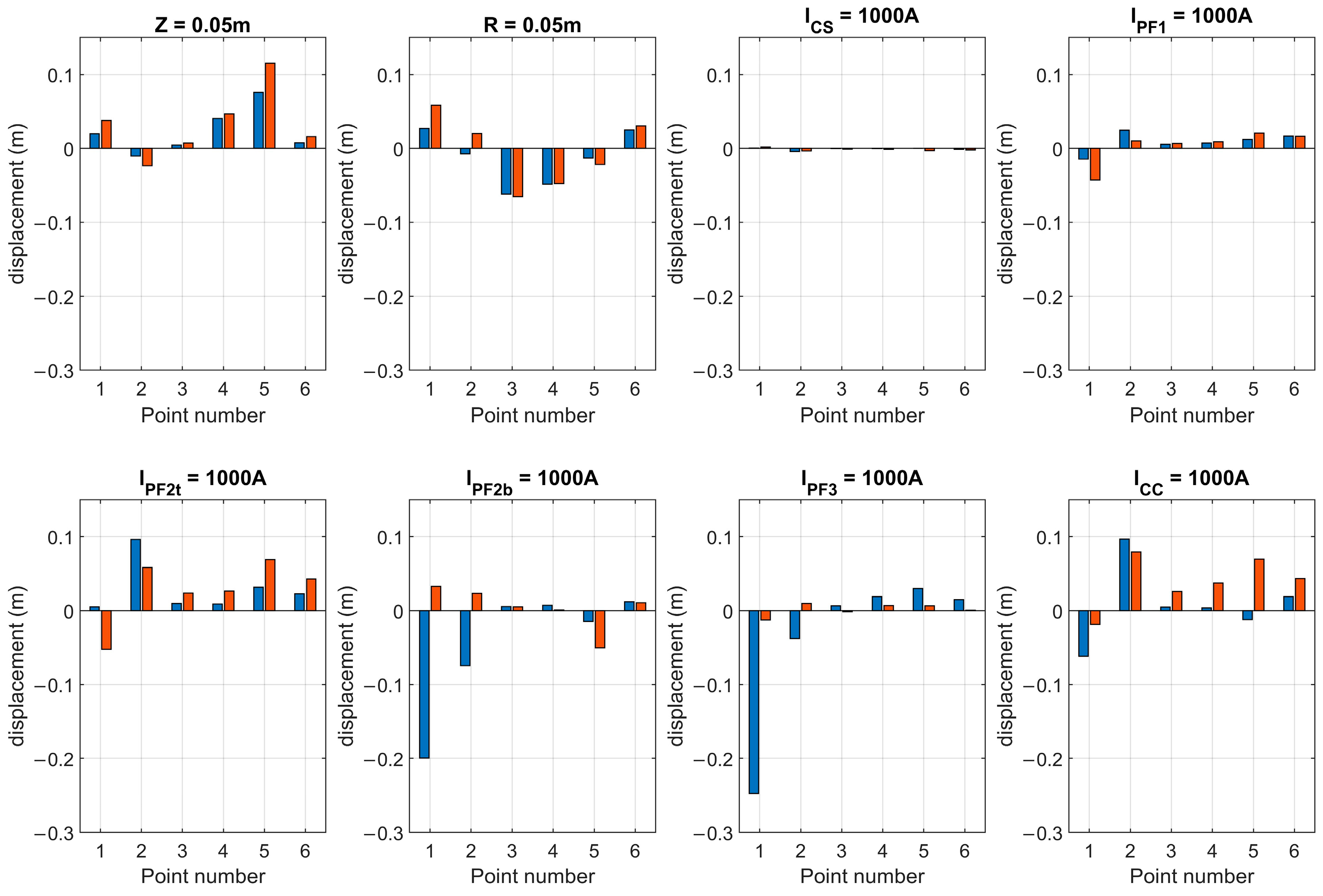
5. Estimation of the Reachability Area of the Plasma Shape

5.1. Definitions of Plasma Shape Estimations

For the successful operation of D-shaped tokamaks, it is necessary to control the plasma shape using feedback. One needs to hold the plasma separatrix near the first wall of the VV. In Globus-M/M2 tokamaks, PF-coils are used for plasma shape control (Figure 2 and Figure 3), but the HFC and the VFC also influence the plasma shape. Estimating the reachability area is performed using the matrix relationship between the inputs and outputs in a steady-state regime. The relationship is obtained from the state–space model of the plant, with all control loops and PID-controllers in them:

$$\begin{array}{c}\dot{x}(t)=Ax(t)+Bu(t),\\ y(t)=Cx(t);\\ x\in {ℝ}^{42}, u\in {ℝ}^8, y\in {ℝ}^6, A\in {ℝ}^{42\times 42}, B\in {ℝ}^{42\times 8},C\in {ℝ}^{6\times 42}.\end{array}$$

(20)

Assuming that derivatives in (20) are equal to zero (because the steady-state regime is considered), the following expression can be investigated:

$$\dot{x}=0=Ax+Bu \Rightarrow x=-A^{-1}Bu; y=Cx=\underset{M}{\underbrace{-C{A}^{-1}B}}u=Mu.$$

(21)

The M-matrix is the sensitivity of the output signals to changes in inputs (Figure 11). This shows how each input signal (Z, R, I_CS, I_PF1, I_PF2t, I_PF2b, I_PF3, I_CC) influences different outputs (P1–P6). Because the reachability area of the plasma shape is multivariable, the problem of its estimation was divided into upper and lower estimations.

The upper estimation of each gap is the maximal absolute value of this gap, which is independent of other gaps (values of other gaps do not matter).

The lower estimation is the maximal simultaneous absolute value of all gaps (all gaps have the same value).

The limits on the plasma position references are 5 cm, and the limits on the references of the PF-currents are 1000 A.

5.2. New Methodology and Upper Estimation of the Reachability Area of the Plasma Shape

The upper estimation is the maximum offset of each gap so that the inputs are within the specified limits. Using (21), the problem of the upper estimation of the ith output is expressed as the following equation:

$$\begin{array}{c}{y}_i\to \max \\ s.t. y_i=M_{i}u={\displaystyle \sum _{j=1}^8{M}_{i,j}{u}_j}, \\ \left|u_j\right|<u_{j\max }, j=\overline{1,8},\end{array}$$

(22)

where $M_i$ is the ith row of matrix $M$. To maximize the sum, ${\displaystyle \sum _{j=1}^8{M}_{i,j}{u}_j}$, it is necessary and sufficient to maximize each term because all the terms are independent. This is achieved using the following equation:

$$u_j=sign\left(M_{i,j}\right)u_{j\max }$$

(23)

Substituting the result of (23) into (22), the maximal possible displacement of the ith gap can be calculated by the expression

$$y_{i\max }={\displaystyle \sum _{j=1}^8{M}_{i,j}sign(M_{i,j})u_{j\max }}.$$

(24)

Using (24), the upper estimation was made of all six gaps of the plasma separatrix for six shots, as in Section 3. The results are shown in Figure 12.

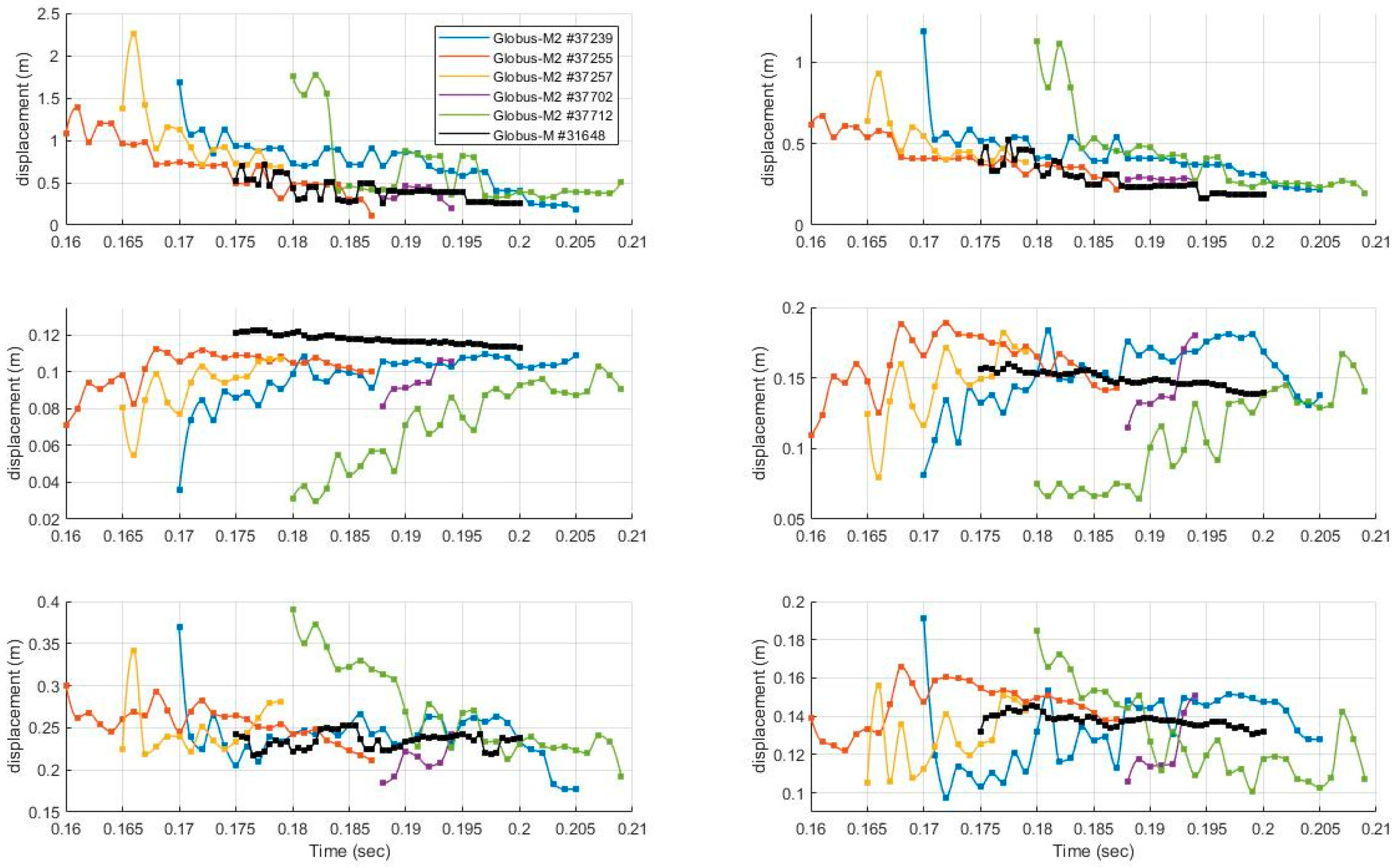
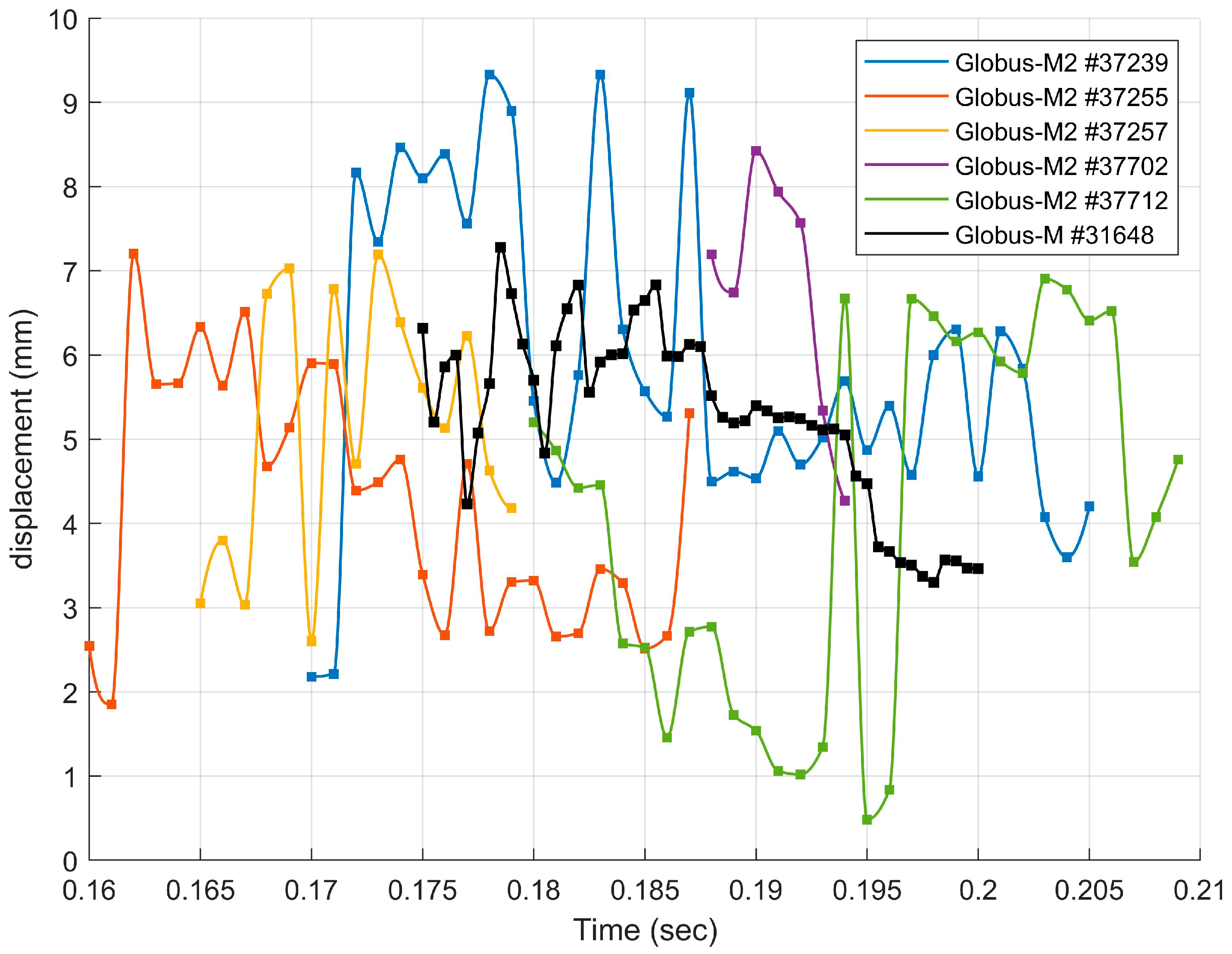
5.3. Methodology and Lower Estimation of the Reachability Area of the Plasma Shape

The lower estimation is obtained with the help of the auxiliary estimation [22].

The auxiliary estimation is the maximal displacement of each gap so that other gaps are equal to zero.

For example, to obtain the auxiliary estimation for gap g₁, it is necessary to find the maximal displacement of this gap, $y_1=M_{1}u$; other gaps (g₁–g₆) are equal to zero, and all inputs u are less than the allowable limits:

$$\begin{array}{c}{y}_1\to \max \\ s.t. y=Mu, y_i=0, i=\overline{2,6}, \\ \left|u_j\right|<u_{j\max }, j=\overline{1,8}.\end{array}$$

(25)

To obtain the auxiliary estimation, matrix $M\in {ℝ}^{6\times 8}$ was divided into two matrices, $M_1\in {ℝ}^{6\times 2}$ and $M_2\in {ℝ}^{6\times 6}$; similarly, the plasma position references were separated from the following PF-current references: $u\in {ℝ}^8, u={[u^T{}_1 , u^T{}_2]}^T, u_1\in {ℝ}^2, u_2\in {ℝ}^6$. This allows us to reverse the square matrix $M_2$:

$$y=Mu=M_1{u}_1+M_2{u}_2 \Rightarrow u_2=M_2^{-1}(y-M_1{u}_1).$$

(26)

Further output signals are defined in the form of $y={\left[0,\dots ,0,y_i,0,\dots ,0\right]}^T$; all possible values of inputs $u_1\in R^2$ are listed and the values of $u_2$ obtained by (26) are tested for admissibility. With the help of a binary search (similar to Section 3), the maximum possible displacements of each gap ($y_i$) show that other gaps are equal to zero and can be obtained. The complexity of each gap estimation is $O(N^{2}lo{g}_2(N))$, where $N$ is the number of nodes in the split in order to iterate over the references.

The disadvantages of this approach are high computational complexity and low accuracy because this approach requires brute force. Another way to calculate the auxiliary estimation is linear programming [25]. The linear programming approach solves problem (25) analytically. The problem may be represented in the standard form, consisting of a linear function to be maximized with linear problem constraints and non-negative variables:

$$\begin{array}{c}f(x_1,\dots ,x_n)=c_1{x}_1+\dots +c_n{x}_n\to \max ;\\ s.t. a_{11}{x}_1+\dots +a_{1n}{x}_n\le b_1;\\ \dots \\ a_{m1}{x}_1+\dots +a_{mn}{x}_n\le b_m;\\ x_1\ge 0,\dots ,x_n\ge 0.\end{array}$$

(27)

In addition, the standard Formula (27) may be represented in a matrix form:

$$\max \left\{c^{T}x\right|s. t. Ax\le b , x\ge 0\}.$$

(28)

By dividing the inputs to two non-zero variables, $u_i=x_i-x_{n+i}$, where $n=8$ is the number of inputs, problem (25) transitions to the standard formula:

$$\begin{array}{c}{y}_1=M_{1,1}{x}_1+M_{1,2}{x}_2+\dots +M_{1,8}{x}_8-M_{1,1}{x}_9-M_{1,2}{x}_{10}-\dots -M_{1,8}{x}_{16}\to \max ,\\ s. t. M_{i,1}{x}_1+M_{i,2}{x}_2+\dots +M_{i,8}{x}_8-M_{i,1}{x}_9-M_{i,2}{x}_{10}-\dots -M_{i,8}{x}_{16}=0, \overline{i=2,6},\\ \begin{array}{c}{x}_j-x_{n+j}\le u_{j\max },\\ -x_j+x_{n+j}\le u_{j\max },\end{array} j=\overline{1,8}\\ x_k\ge 0, k=\overline{1,16.}\end{array}$$

(29)

Problem (29), equivalent to (27) and (28), is solved using the simplex method [25]. To explain how the simplex method works, geometric interpretation can be used. Problem constraints are half-spaces. In sum, the constraints denote a convex polyhedron, and it is necessary to find a point in it where the functional value is at its maximum. It is possible to show that the solution is one of the corner points. Each iterative step of the method is the transition from one corner point to the adjacent, at which the value of the function grows. The criterion of algorithm stopping is finding such a point where, in all the adjacent corner points, the functional value is lower than in the current point [25].

Solving (29) for gap P1 at 185 ms of shot #37239, the maximum displacement with other gaps equal to zero can be obtained. It is 116 mm. It is achieved with position references equal to −20 mm vertically and −1 mm horizontally and currents references in six PF-coils: 1000 A, 1000 A, 625 A, 520 A, 1000 A, and 454 A for CS, PF1, PF2 top, PF2 bottom, PF3, and CC, respectively.

Similarly, it is possible to make the auxiliary estimation for each gap using the simplex method. After that, it is necessary to move from the auxiliary estimation of each gap to the lower estimation, i.e., the maximal displacement that all gaps could achieve simultaneously with the input signals in allowable limits:

$$y_{\max }: \forall y\in R^6:\left|y_i\right|\le y_{\max }, i=\overline{1,6}, y=Mu, \left|u_j\right|\le u_{j\max }, j=\overline{1,8}.$$

(30)

If $y_{i \max }$ is the auxiliary estimation of the ith gap, then it is possible to simultaneously put each gap in limits $a_i{y}_{i\max }\ge 0, i=\overline{1,6}$, provided that $1\ge {\displaystyle \sum _{i=1}^6{a}_i}$. This can be shown with the help of the linearity of the matrix multiplication:

$$\begin{array}{c}y={[a_1{y}_{1\max }, a_2{y}_{2\max },\dots ,a_6{y}_{6\max }]}^T=\\ =a_1{[y_{1\max },0,\dots ,0]}^T+a_2{[0,y_{2\max },0,\dots ,0]}^T+\dots +a_6{[0,\dots ,0,y_{6\max }]}^T\end{array}$$

(31)

Because $y_{i \max }$ is the auxiliary estimation, then

$${[0,\dots ,0,y_{i\max },0,\dots ,0]}^T=M{u}^i, u^i\in R^8, \left|u_j^i\right|\le u_{j\max }.$$

(32)

The upper index is used for matching input signals and the gap number that this input displaces. Substituting (31) and (32) into (30), one obtains the following equation:

$$y=Mu=M{{\displaystyle \sum _{i=1}^6{a}_i{u}^i=M\left[{\displaystyle \sum _{i=1}^6{a}_i{u}_1^i}, {\displaystyle \sum _{i=1}^6{a}_i{u}_2^i},\dots ,{\displaystyle \sum _{i=1}^6{a}_i{u}_8^i},\right]}}^T.$$

(33)

The first component of the input signal is within the allowable limits: $u_1={\displaystyle \sum _{i=1}^6{a}_i{u}_1^i\le u_{1\max }}$. Using ${\displaystyle \sum _{i=1}^6{a}_i\le 1, u_1^i\le u_{1\max }}, u_1^i\le u_{1\max }$, we come to the following nonstrict inequality:

$$u_1={\displaystyle \sum _{i=1}^6{a}_1{u}_1^i}\le {\displaystyle \sum _{i=1}^6{a}_1{u}_{1\max }^i}=u_{1\max }^i\underset{\le 1}{\underbrace{{\displaystyle \sum _{i=1}^6{a}_1}}}\le u_{1\max }^i.$$

(34)

Thus, the first component of the input signal is within the allowable limits. Similarly, in (34), each component of the input is also within the allowable limits. For the estimation of $y_{\max }$, it is enough to choose

$$a_i: y_{\max }=a_i{y}_{i\max }, {\displaystyle \sum _{i=1}^6{a}_i}=1.$$

(35)

Solving (35), we obtain the following equation:

$$y_{\max }={\left({\displaystyle \sum _{i=1}^6{y}_{i\max }^{-1}}\right)}^{-1}.$$

(36)

The result of (36) can be verified by the following substitution:

$$\begin{array}{c}{a}_i={\left(y_{i\max }{\displaystyle \sum _{j=1}^6{y}_{j\max }^{-1}}\right)}^{-1},\\ {{\displaystyle \sum _{i=1}^6{a}_i={\displaystyle \sum _{i=1}^6{\left(y_{i\max }{\displaystyle \sum _{j=1}^6{y}_{j\max }^{-1}}\right)}^{-1}= }\left({\displaystyle \sum _{j=1}^6{y}_{j\max }^{-1}}\right)}}^{-1}{\displaystyle \sum _{i=1}^6{y}_{i\max }^{-1}=1.}\end{array}$$

(37)

Summarizing all of the above, the auxiliary estimation is the solution to the linear programming problem, which was solved by the simplex method; reversing the sum of the reversed auxiliary estimations (37) is the lower estimation for each moment of each shot.

For example, at 185 ms of shot #37239 of the Globus-M2 spherical tokamak, the lower estimation of the reachability area is 5.4 mm; i.e., all gaps, g₁–g₆, could take any values in a range from −5.4 mm to 5.4 mm, with inputs within allowable limits (a position displacement less than 5 mm and currents in PF-coils less than 1000 A).

By solving (29)–(36), the lower estimations of the reachability region of the plasma can be obtained for five shots of Globus-M2 and one shot of Globus-M, as shown in Figure 13. The advantage of the simplex method over the coarse force method using (26) is the increased accuracy and reduced time costs. Simplex method calculations are about 100 times faster.

6. Conclusions

The preparations of the plasma shape control system for the Globus-M2 tokamak were performed to apply a new methodology of plasma shape estimation. For that application, PID-controllers were synthesized using the QFT method. A numerical simulation shows that they stabilize the system with plasma models for various plasma shots. Analytical and numerical estimations of the vertical controllability area provided equivalent results. For tokamaks Globus-M and Globus-M2, these values are similar and are about 15 cm.

The controllability region of the unstable vertical plasma position rapidly changes during shots and from shot to shot. Its value is about 10 cm (Figure 9). Because the plasma column height is about 60–80 cm, and the VV height is 1 m (Figure 1), the plasma can be controlled over almost the entire height of the VV.

The reachability area was estimated for both tokamaks. It is shown that the current in the central solenoid provides a minimal influence on the plasma shape (Figure 11). The current in the PF3 coil in Globus-M2 has more influence on the plasma shape than the same current in Globus-M. The lower reachability estimation is about 1 cm; the upper reachability estimation is about 10–20 cm.

The reachability area of the plasma shape for each gap is about 1–10 cm; consequently, the development of a plasma shape feedback control system is possible. In Figure 11, the influence of each PF-coil on the plasma shape is shown. All coils, besides the central solenoid, have a noticeable influence on the plasma shape; consequently, it is important to develop a multivariable plasma shape control system on the basis of PF-coils without a central solenoid in the feedback, which should primarily control the plasma current.

References

1. Wesson, J. Tokamaks, 3rd ed.; Clarendon Press: Oxford, UK, 2004. [Google Scholar]
2. Mitrishkin, Y.; Korenev, P.; Prokhorov, A.; Kartsev, N.; Patrov, M. Plasma Control in Tokamaks. Part 1. Controlled thermonuclear fusion problem. Tokamaks. Components of control systems. Adv. Syst. Sci. Appl. 2018, 18, 26–52. [Google Scholar]
3. Mitrishkin, Y.V.; Kartsev, N.M.; Pavlova, E.A.; Prohorov, A.A.; Korenev, P.S.; Patrov, M.I. Plasma Control in Tokamaks. Part. 2. Magnetic Plasma Control Systems. Adv. Syst. Sci. Appl. 2018, 18, 39–78. [Google Scholar]
4. Mitrishkin, Y.; Kartsev, N.; Konkov, A.; Patrov, M. Plasma Control in Tokamaks. Part 3.1. Plasma magnetic control systems in ITER and DEMO. Adv. Syst. Sci. Appl. 2020, 2, 82–97. [Google Scholar]
5. Mitrishkin, Y.; Kartsev, N.; Konkov, A.; Patrov, M. Plasma Control in Tokamaks. Part 3.2. Simulation and realization of plasma control systems in ITER and constructions of DEMO. Adv. Syst. Sci. Appl. 2020, 20, 136–152. [Google Scholar]
6. Gryaznevich, M.P.; A Chuyanov, V.; Kingham, D.; Sykes, A.; Tokamak Energy Ltd. Advancing fusion by innovations: Smaller, quicker, cheaper. J. Phys. Conf. Ser. 2015, 591, 012005. [Google Scholar] [CrossRef] [Green Version]
7. Chuyanov, V.A.; Gryaznevich, M.P. Modular fusion power plant. Fusion Eng. Des. 2017, 122, 238–252. [Google Scholar] [CrossRef]
8. Lawson, J.D. Some Criteria for a Power Producing Thermonuclear Reactor. Proc. Phys. Soc. Sect. 1957, 70, 6–10. [Google Scholar] [CrossRef]
9. Gusev, V.; Azizov, E.; Alekseev, A.; Arneman, A.; Bakharev, N.; Belyakov, V.; Bender, S.; Bondarchuk, E.; Bulanin, V.; Bykov, A.; et al. Globus-M results as the basis for a compact spherical tokamak with enhanced parameters Globus-M2. Nucl. Fusion 2013, 53, 093013. [Google Scholar] [CrossRef]
10. Minaev, V.; Gusev, V.; Sakharov, N.; Varfolomeev, V.; Bakharev, N.; Belyakov, V.; Bondarchuk, E.; Brunkov, P.; Chernyshev, F.; Davydenko, V.; et al. Spherical tokamak Globus-M2: Design, integration, construction. Nucl. Fusion 2017, 57, 066047. [Google Scholar] [CrossRef]
11. Humphreys, D.; Casper, T.; Eidietis, N.; Ferrara, M.; Gates, D.; Hutchinson, I.; Jackson, G.; Kolemen, E.; Leuer, J.; Lister, J.; et al. Experimental vertical stability studies for ITER performance and design guidance. Nucl. Fusion 2009, 49, 115003. [Google Scholar] [CrossRef] [Green Version]
12. Mitrishkin, Y.V.; Kartsev, N.V.; Zenkov, S.M. Stabilization of unstable vertical position of plasma in T-15 tokamak. Autom. Remote Control 2014, 75 Pt 1, 281–293. [Google Scholar] [CrossRef]
13. Mitrishkin, Y.V.; Korenev, P.S.; Konkov, A.E.; Kartsev, N.M.; Smirnov, I.S. New horizontal and vertical field coils with optimised location for robust decentralized plasma position control in the IGNITOR tokamak. Fusion Eng. Des. 2022, 174, 112993. [Google Scholar] [CrossRef]
14. Mitrishkin, Y.V.; Prokhorov, A.A.; Korenev, P.S.; Patrov, M.I. Hierarchical robust switching control method with the equilibrium reconstruction code based on Improved Moving Filaments approach in the feedback for tokamak plasma shape. Fusion Eng. Des. 2019, 138, 138–150. [Google Scholar] [CrossRef]
15. Kuznetsov, E.A.; Mitrishkin, Y.V.; Kartsev, N.M. Current Inverter as Auto-Oscillation Actuator in Applications for Plasma Position Control Systems in the Globus-M/M2 and T-11M Tokamaks. Fusion Eng. Des. 2019, 143, 247–258. [Google Scholar] [CrossRef]
16. Korenev, P.S.; Mitrishkin, Y.V.; Patrov, M.I. Reconstruction of equilibrium distribution of tokamak plasma parameters by external magnetic measurements and construction of linear plasma models. Mechatron. Autom. Control 2016, 17, 254–265. (In Russian) [Google Scholar] [CrossRef]
17. Qiu, Q.; Guo, Y.; Gao, L.; Huang, J.; Sun, H.; Lin, X.; Li, J.; Xiao, B.; Liu, L.; Luo, Z.; et al. The numerical analysis of controllability of EAST plasma vertical position by TSC. Fusion Eng. Des. 2019, 141, 116–120. [Google Scholar] [CrossRef]
18. Ou, Y.; Schuster, E. Controllability analysis for current profile control in tokamaks. In Proceedings of the 48h IEEE Conference on Decision and Control (CDC) held jointly with 2009 28th Chinese Control Conference, Shanghai, China, 15–18 December 2009; pp. 315–320. [Google Scholar]
19. Maviglia, F.; Artaserse, G.; Albanese, R.; Calabrò, G.; Crisanti, F.; Pironti, A.; Pizzuto, A.; Ramogida, G. Poloidal field circuits sensitivity studies and shape control in FAST. Fusion Eng. Des. 2011, 86, 1076–1079. [Google Scholar] [CrossRef]
20. Garcia-Sanz, M. Robust Control Engineering. Practical QFT Solutions; Taylor & Francis Group, CRC Press: Boca Raton, FL, USA, 2017. [Google Scholar]
21. Dorf, R.C.; Bishop, R.H. Modern Control Systems. Solution Manual, 11th ed.; Prentice Hall: Upper Saddle River, NJ, USA, 2008. [Google Scholar]
22. Mitrishkin, Y.V.; Kruzhkov, V.I.; Patrov, M.I. Estimation of controllability region of unstable vertical plasma position and plasma separatrix multivariable reachability area of a spherical tokamak. In Proceedings of the 46th EPS Conference on Plasma Physics, Milan, Italy, 8–12 July 2019. [Google Scholar]
23. Kahaner, D.; Moler, D.; Nash, S. Numerical Methods and Software; Prentice Hall: Upper Saddle River, NJ, USA, 1988. [Google Scholar]
24. Garcia-Sanz, M. The QFT Control Toolbox for Matlab—QFTCT. 2018. Available online: http://codypower.com (accessed on 13 October 2022).
25. Dantzig, G.B.; Orden, A.; Wolfe, P. Generalized Simplex Method for Minimizing a Linear Form Under Linear Inequality Restraints. Pac. J. Math 1955, 5, 183–195. [Google Scholar] [CrossRef]
Figure 1. Globus-M2 tokamak.
Mathematics 10 04605 g001
Figure 2. (a) Poloidal system; (b) equal level lines of poloidal magnetic flux in vertical cross-section of Globus-M/M2 and points P1–P6 for the gap control with a lower X-point and (c) upper X-point.
Mathematics 10 04605 g002
Figure 3. Block diagram of the Globus-M/M2 plasma control system.
Mathematics 10 04605 g003
Figure 4. Set of Nichols diagrams of an open-loop system with plasma models corresponding to different moments in time with PID-controllers tuned with QFT.
Mathematics 10 04605 g004
Figure 5. Changes in stability margins during a plasma discharge. Circles denote the minimums of the phase and amplitude margins in this system. Here and below, solid lines between circles were obtained with the PCHIP approach, (7) and (8) [23].
Mathematics 10 04605 g005
Figure 6. Step responses of closed-loop systems with a plasma model corresponding to 185 ms of shot #37239 with nonlinear current inverter models [15] and PID-controllers (9), tuned with the QFT methodology.
Mathematics 10 04605 g006
Figure 7. (a) Step responses of the vertical plasma position in the system with and without the pre-filter. Overshot is decreased from 29% to 17%, setting time is decreased from 7 ms to 5 ms; (b) set of 18 step responses of the vertical and horizontal plasma control systems with different plasma models.
Mathematics 10 04605 g007
Figure 8. Block diagram of the system for the numerical estimation of the vertical plasma position controllability region.
Mathematics 10 04605 g008
Figure 9. (a) Estimation of the vertical controllability area during the different shots of the Globus-M/M2 spherical tokamaks. Points correspond to the minimal vertical controllability area during the divertor phase of each shot. (b) The controllability area limits and phase trajectory projections on the plane (IHFC, Z) for the Globus-M2 model at 197 ms of shot #37712 at a maximum of 900 V and a minimum of −900 V on HFC. Circles denote points in the controllability area; x marks denote points out of the controllability area; green shading corresponds to the controllability area (18). (c) Minimal controllability area during shots on the plane (IHFC, Z).
Mathematics 10 04605 g009
Figure 10. (a) Results of the system simulations with different initial vertical plasma displacements and maximum voltages on the HFC. (b) Principle of the binary search algorithm to find the controllability region. Red points are initial displacements out of the controllability region and blue points are inside the controllability region. Step by step, the limit of the controllability region estimation accuracy grows. The accuracy increases up two times at each step.
Mathematics 10 04605 g010
Figure 11. Sensitivity of plasma shapes, namely, gaps, to the references of the plasma position and the currents in the PF-coils for shot #37239 of tokamak Globus-M2 versus shot #31648 of Globus-M at 185 ms. Histograms show a strong connection between plasma position and plasma shape, a weak influence from the central solenoid current on the plasma shape, and a strong cross-influence from the PF-coils currents on the plasma shape’s projections, P1–P6.
Mathematics 10 04605 g011
Figure 12. Changes in the upper estimation of the plasma shape during different shots of the spherical Globus-M/M2 tokamaks.
Mathematics 10 04605 g012
Figure 13. Dynamic of the lower estimation of the reachability region of plasma shape changes during different shots in spherical tokamak Globus-M/M2.
Mathematics 10 04605 g013
Publisher’s Note: MDPI stays neutral with regard to jurisdictional claims in published maps and institutional affiliations.