Article

Contactless Determination of a Permanent Magnet’s Stable Position within Ferrofluid

Faculty of Electrical Engineering and Computer Science, University of Maribor, Koroska cesta 46, 2000 Maribor, Slovenia
*
Author to whom correspondence should be addressed.
Mathematics 2022, 10(14), 2499; https://doi.org/10.3390/math10142499
Submission received: 31 May 2022 / Revised: 15 July 2022 / Accepted: 16 July 2022 / Published: 18 July 2022
(This article belongs to the Section Mathematical Physics)

Abstract

:
The paper deals with the contactless detection of a rod permanent magnet’s position within a ferrofluid. The working principle of the proposed approach is grounded on the solenoidal nature of the field lines. For the line detection technique analyzed in this article, where the magnetic field is scanned along the line parallel to the magnet’s axial direction, the center of the magnet corresponds to the point on the line where the radial component of the magnetic field vanished. The concept introduced here was evaluated numerically, where the results showed a promising perspective for the technique to be employed in practice. In contrast to the X-ray or Vernier-caliper-based technique, the one proposed here is somewhat more suitable for employment in applications where simplicity and robustness are of vital importance.

1. Introduction

Ferrofluid-based devices and applications have captured the attention of many researchers around the globe. This artificial magnetically sensitive liquid substance exhibits some special properties when it is exposed to a magnetic field, and thus it has found its place in some promising applications, such as dampers [1,2,3,4,5], accelerometers [6,7,8], vibration absorbers [9,10,11,12,13,14], and various sensors [15,16,17].
Especially attractive for practical adoption is the self-levitation phenomenon that occurs with the permanent magnet (PM) immersed in a ferrofluid. The phenomenon was first observed and reported by Rosensweig in 1966 [18,19], and it is known under the term second-order buoyancy (SOB). Through the years, the SOB was studied theoretically and experimentally. The main focus of the researchers in the field was devoted to the evaluation of the SOB force. Some recent and relevant research studies covering the topic are enlisted in the references and discussed briefly below.
One of the first attempts to evaluate the second-order buoyancy force numerically was reported in the work of Yang et al., where the force calculation was performed through the current image method and finite element method (FEM) [20,21]. FEM-based calculation and experimental verifications of SOB can be also found in the work of Qian et al. [7], where the SOB was measured with the dynamometer and Vernier caliper attached rigidly to the PM. It is somewhat worth mentioning that the early stage SOB force measurement technique was based on the tensile force of the rope attached to the top of the magnet within the ferrofluid [22]. A series of scientific reports published by Yu and some other authors were dedicated to extensive theoretical consideration of SOB, but the experimental setup was still based on the Dynamometer and Vernier caliper [8,23,24,25].
Even though the SOB phenomenon has been well covered by theory and by experiments, there is always space left for some new ideas. The technique used so far in the force measurements is purely mechanical, for which a rigid connection is required between the PM and the dynamometer. Such a construction solution can pose a concrete issue when the suitable design of the SOB device is in question. On the other hand, the sensitive measurement equipment that comes with such a measuring technique is not applicable in heavy working conditions; thus, the alternative method for PM position detection and SOB force evaluation seems to be more than welcome.
To fill the gap in the field, a novel magnetically based technique for detecting the PM’s position within the ferrofluid is presented in the article. Instead of the caliper, the magnetic sensor placed in the air near the magnet is used to detect the magnet’s levitation height. The sensor should be able to move vertically, or, in general, parallel to the magnetization direction of the PM. The key concept of the technique is grounded on the solenoidal nature of magnetic field lines; therefore, the center of the PM is determined at the point where the radial component of the magnetic field equals zero. Moreover, the approach demands no physical connection between the sensor and magnet. Although the proposed technique was originally devoted to the detection of the magnet’s levitation height it can be adopted to evaluate the SOB force as well. To do that, the magnet’s geometry and density should be known in advance, along with the density of the ferrofluid, and, afterward, the calculation of the SOB is straightforward [26]. The simulation-based results presented in this article predict a promising perspective for the technique to be employed in practice.
In this paper, the magnetic field distribution in the space is calculated by the FEM software, where a two-dimensional axisymmetric model is used in cylindrical coordinates. Although FEM is the most widely used numerical method in computational electromagnetics, other methods can also be employed for computation. For instance, in cases where the system is very sensitive, the spectral element method (SEM) could be utilized to obtain better accuracy [27,28,29,30].

2. Materials and Methods

As mentioned in the introduction, a novel contactless magnetic-based technique is proposed to determine the PM’s position. To bring a clear and understandable physical picture to the reader, the following theoretical consideration should be discussed first.
Imagine for the moment an empty cylindrical container with a cylindrical PM placed in it, as depicted in Figure 1. For simplicity, let us assume that the magnetic symmetry exists along the φ direction. Now, if the magnetic field distribution along the z-axis at a distance a from the magnet’s center is in question, it can be measured by bringing the magnetic field sensor to the desired point. While the magnetic field is a vector quantity, it is somewhat desired to have a sensor able to pick up all three fields’ components. Presume the experimental setup such that the sensor starts scanning the field at point 1 and ends at point 5 (the sensor is moving solely along the vertical position). However, at a specific sensor position, only the z component will remain due to the solenoidal nature of the magnetic field. In other words, the point where the radial component of the magnetic field vanishes lies in the plane which goes through the PM’s center. In the magnetic sense, it represents the plane normal to the field lines. Following the presented physical picture, it can easily be deduced that the magnet’s position can be determined by virtue of the magnetic field distribution in the space.

2.1. Theoretical Background

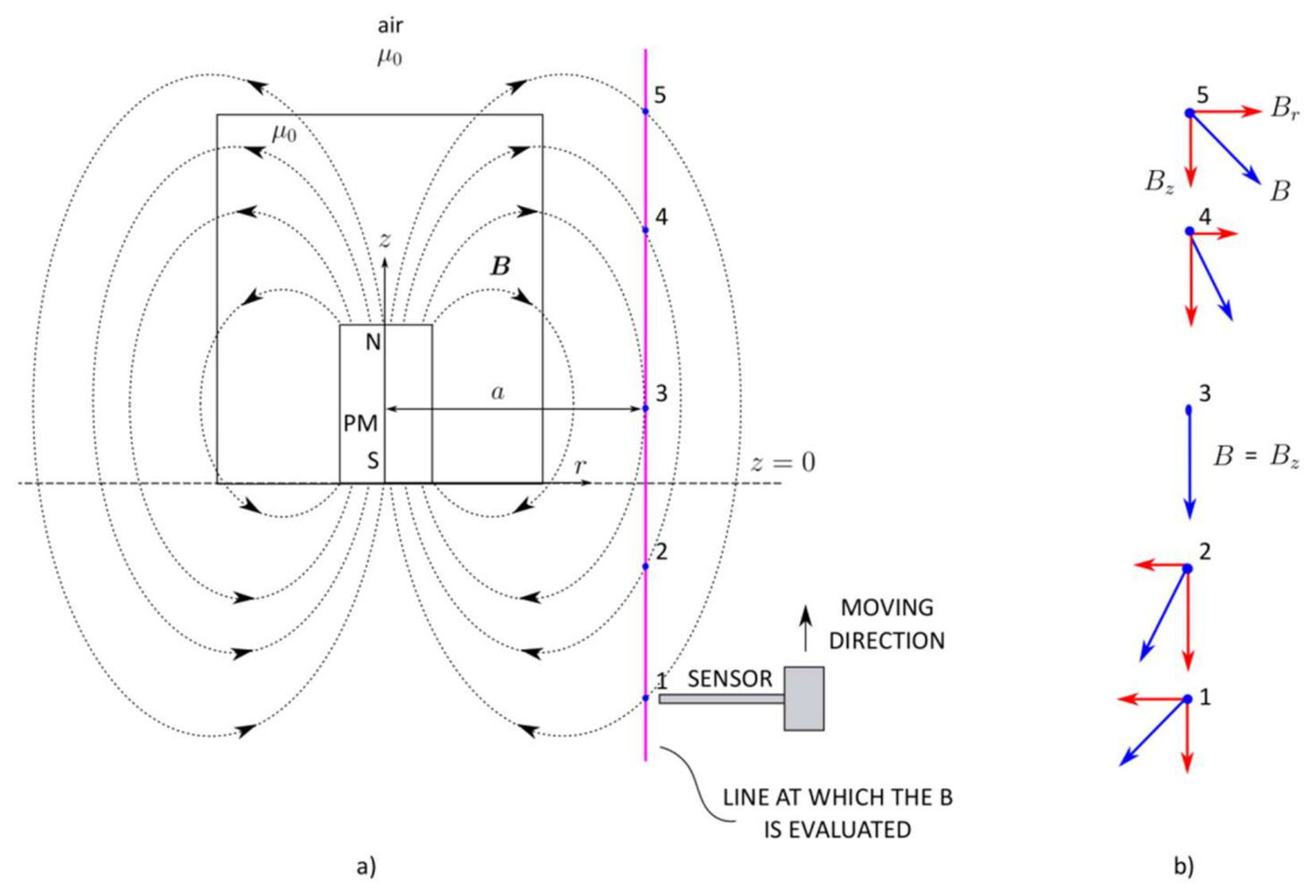
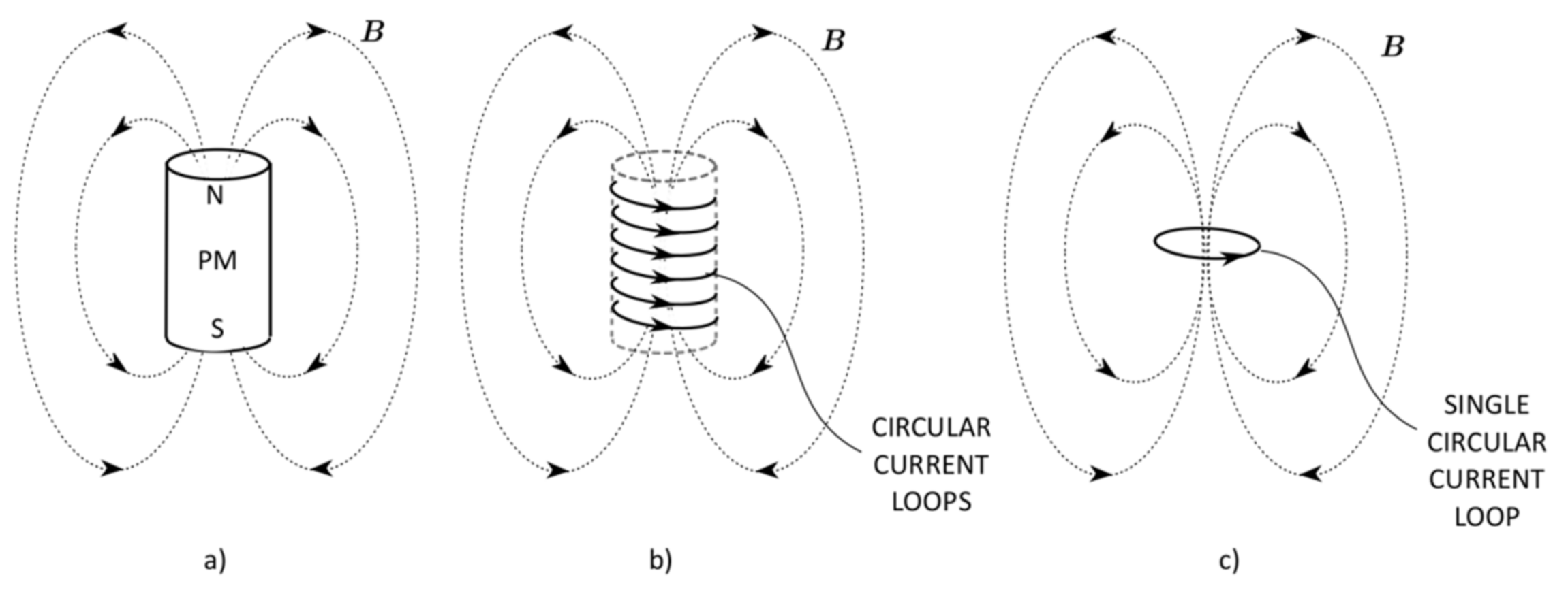
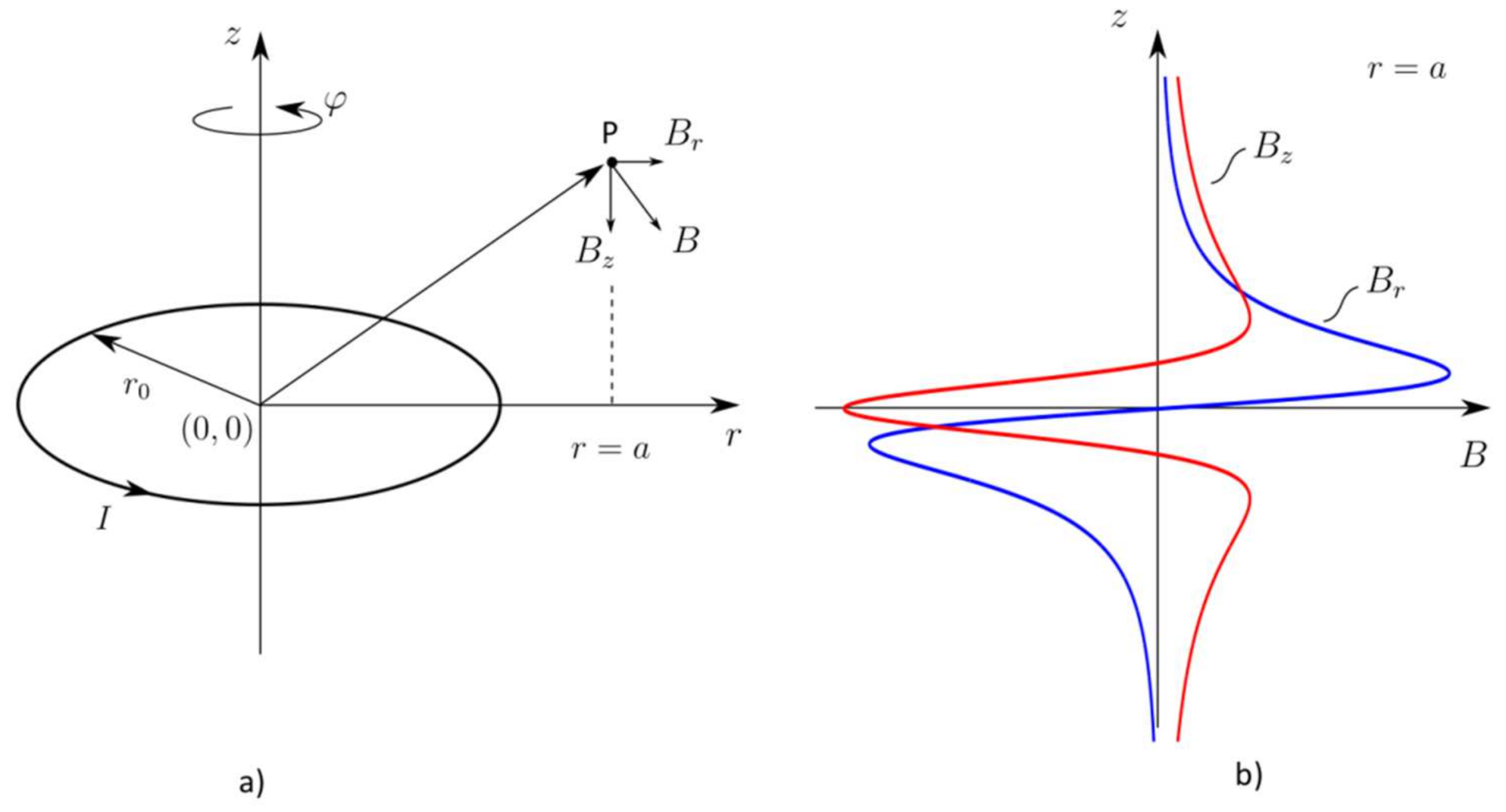
2.1.1. Permanent Magnet in Nonmagnetic Media

To satisfy the formality, a brief mathematical formulation of the aforementioned physical abstraction is derived in the following section. The magnetic field produced in the space by the PM (Figure 2a) can also be presented as a field evoked by the current loops, as shown in Figure 2b. For simplicity, let us consider a PM model equivalently described only by a single circular steady current loop (Figure 2c). Referring to electromagnetic theory, a magnetic field density around such a structure is defined straightforwardly by Equations (1) and (2) [31].
B r = μ 0 I 4 π   1 r 0 + r 2 + z 2   z r   2 m 1 m   E m 2 K m
B z = μ 0 I 4 π   1 r 0 + r 2 + z 2     2 K m + E m 1 m   m r 0 + r r 2 ,
where μ 0 is the absolute permeability of the free space; I is a steady current in the loop; r 0 is the radius of the current loop; r is a radial distance component; z is an axial distance component; m is an elliptic integral module defined as m = 4 r 0 r r 0 + r 2 + z 2 ; K m and E m are the complete elliptic integrals of the first and the second kind of argument m , respectively. The geometry arrangement which pertains to Equations (1) and (2) is provided in Figure 3a.
By close examination of Equations (1) and (2) or Figure 3b, it is seen that the radial component of the field vanishes at z = 0 , and the z-component reaches its extreme value there. The magnitudes of the field’s components are illustrated in Figure 3b. The field is evaluated along the line parallel to the z -axis at r = a . Referring back to the setup in Figure 1, the PM’s position can be determined by finding the point on the line along the z-coordinate where B r equals zero and B z attains its extreme value. While the field orientation in a space depends on the current direction (or the direction of magnetization in the case of a PM), the term extreme mentioned in context with B z can refer to a minimum or maximum value.

2.1.2. Permanent Magnet within Ferrofluid

So far in the consideration of the problem, the PM has been surrounded by a nonmagnetic and transparent material, i.e., air, but in the case of the PM immersed in the ferrofluid, the transparency is lost, and the magnet’s position within the ferrofluid is not detectable by the eye. Another phenomenon shows up with the PM immersed in ferrofluid. Namely, the PM’s self-levitation mechanism will appear due to the presence of magnetic fluid pressure in the ferrofluid. Consequently, the magnet will no longer sit on the container’s bottom, but will move vertically to a new stable position at z 0 (Figure 4). Thus, it is somewhat reasonable to expect a change in the magnetic field distribution, i.e., the distribution in Figure 3b will shift higher with respect to the z-coordinate.
Here, the stable PM position can be determined by the nonmagnetic caliper, X-ray [32], or the already discussed magnetic approach. The latter has some promising advantages over the other two, so let us point out some of them. Measuring the magnet’s position by caliper involves a special housing design; the measurement is performed mechanically, and it is much more sensitive to mechanical shocks in operation. Moreover, the whole system should be designed with special care due to all the moving components it consists of. The X-ray method is costly and requires appropriate safety measures; thus, it is somewhat unacceptable for usage in a wide range of applications such as various sensor devices.
On the other hand, ferrofluid is magnetically sensitive material, and its presence in the vicinity of the PM will change the magnetic field distribution to some extent. However, due to the relatively low permeability of ferrofluid, which is moving around 1.2–4 in its relative value, the detection of the magnet’s center can be determined on the same basis as suggested in Section 2.1.1.

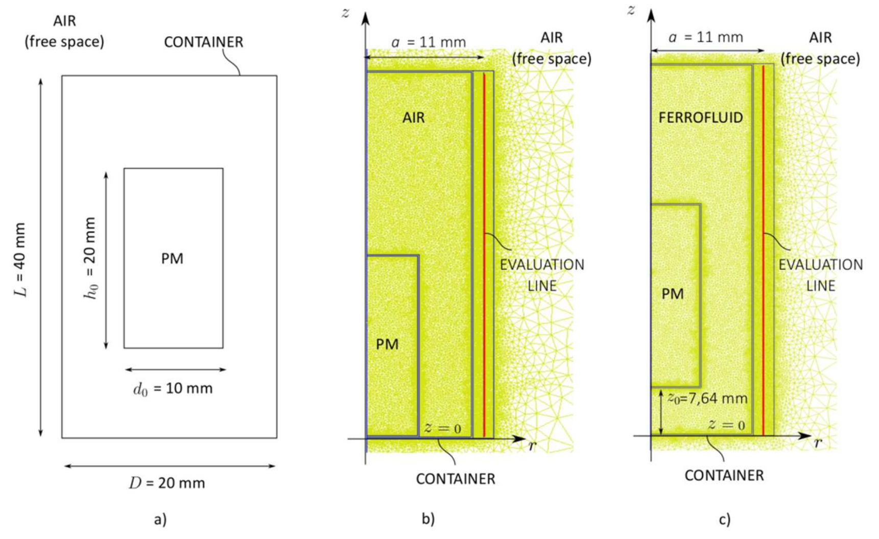
2.2. FEM Model and Simulation Setup

The FEM model of a PM levitating in ferrofluid was built to prove the concept and to visualize the field lines. The simulation setup used in this study is related directly to the research already conducted by the authors of the text, which is well covered, both theoretically and experimentally [26]. For details about the experimental verification, the reader is directed to [23]. However, the model’s dimensions and material properties employed in the presented model corresponded to the ones in [26] (Table 1). Due to the new contactless technique presented here, the nonmagnetic rod that comes with the caliper was no longer required to detect the PM’s position within the ferrofluid; thus, it is omitted from the FEM model.
The 2D axisymmetric magnetostatic model was constructed in the FEMM 4.2 software [33]. In the study, two cases are considered as follows. In the first setup, let us call it case A, the PM was placed at the bottom of the empty container ( z = 0 ), and the magnetic field distribution was evaluated along the straight line outside the container at r = a parallel to the z-coordinate. The second one indicated as case B involved a container filled with ferrofluid where the PM levitated at some stable height z 0 above the container’s bottom, in particular z 0 = 7.64 mm. The magnetic field was evaluated along the same straight line as in case A. The geometrical proportions and virtual experiment setups are shown in Figure 5.
The materials’ properties listed in Table 1 were chosen to fit well with the ones in [23,26]. The meanings of the symbols in Table 1 are as follows: ρ is the material or substance density; μ r is the relative permeability; B r e m and H c are the remanence and coercive force of the PM, respectively; and χ i is the initial magnetic susceptibility defined at low magnetic field intensity. While the PM consists of a rare earth hard magnetic material, its slope in the B-H characteristic is very close to unity. Actually, in reality, the value of the PM’s relative permeability μ r is about 1.05, but the unity value is applied in the simulations to agree with the one in [23]. The mesh size within the PM and container was chosen so as to provide an accurate field approximation, especially because the used software, FEMM 4.2, deals only with the first order triangular elements. To obtain a better accuracy, a very fine mesh was used in the space where the evaluation line was placed. The automatic triangle mesh size option was posed in the outer space (free space) outside the container, as is shown in Figure 5b,c. The total number of elements involved with the FEM model was 38,750.

3. Results and Discussion

A numerical verification of the PM’s position detection based on the proposed technique was generated regarding two cases, case A and case B. In case A, the PM was placed at the bottom of the empty container and its center position was known in advance and corresponded to z = h 0 2 (Figure 5b). By filling the container with ferrofluid, the PM will start to levitate at the equilibrium height z = z 0 , and its center will move towards a higher value to z = h 0 2 + z 0 , which is announced in case B (Figure 5c). The stable levitation height z 0 of the magnet was calculated by the surface integral method (SIM) in FEMM 4.2 software and was deduced from [26].

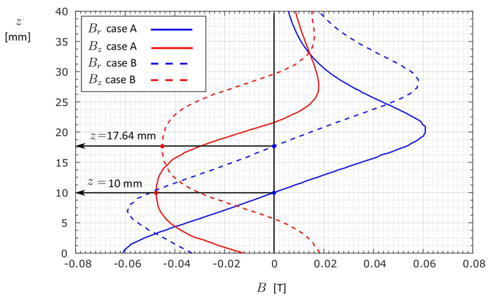
3.1. Position Detection of the PM within an Empty Container—Case A

Simulation of the magnetic field distribution in the free space around the PM within the empty container along with the spatial distribution of the field’s components B r and B z   is given in Figure 6. The field was evaluated along the vertical line 1 mm from the container. The shapes of the curves in the figure apparently corresponded to those predicted by the presented theory. Moreover, from the numerical results, it was evident that the PM center located at z = 10   mm coincided with the point on the evaluation line where B r was equal to zero and B z reached its extreme value. The field distribution revealed more information. Examining the shape of the radial magnetic field component B r in Figure 6, one can see that the PM height h 0 was almost equal the distance between its extreme values. It should be pointed out that the last condition held only for the field evaluated not too far from the magnet, as will be shown with the parametric analysis at the end of the chapter. However, the aforementioned condition was met in most of the applications of interest.

3.2. Position Detection of the PM within a Ferrofluid-Filled Container—Case B

Simulation of the magnetic field distribution in the space around the PM immersed in ferrofluid (case B) was executed similarly as in case A already discussed. The numerical results presented in Figure 7 show that the magnet’s center coincided with the points in the graph located at z = 17.64   mm , where B r = 0 and B z = B z , m i n , which was somewhat the expected outcome. The PM’s height h 0 can also be evaluated through the B r curve by measuring the distance between its extremes, as was observed in case A. The levitation altitude z 0 was then located, considering the magnet’s height as z 0 = z h 0 2 , which resulted in z 0 = 7.64   mm .
The comparison of the results for both cases is given in Figure 8. The solid and the dashed lines pertain to case A and B, respectively. The levitation height z 0 occurred as the difference between the B r zero-cross points. The effect of the ferrofluid’s permeability is also observable in the figure, where case B came with slightly lower values than case A. In general, this contrast was intensified by the difference in the permeability of the substance surrounding the PM.
Even though the interpretation of results can be brought on graphical bases as depicted in Figure 8, the mathematical explanation was delivered by considering the PM’s representation as a single current loop (Figure 3). In this case, Equations (1) and (2) should be examined in more detail. The zero-cross point of the radial magnetic field component is apparent from Equation (1). By replacing the global z coordinate with the local one = z ξ 0 in Equation (1), the B r vanished at z = ξ 0 ( ξ 0 indicates the distance between the PM’s center and the container’s bottom). Some more mathematical effort should be employed to explain the extreme of B z at z = ξ 0 . Here, it is convenient to rewrite Equation (2) as a product of two functions α and β , i.e., B z = α β , where α = μ 0 I 4 π   1 r 0 + r 2 + ξ 2 , β = 2 K m + E m 1 m   m r 0 + r r 2 , and ξ = z ξ 0 . Now, the condition for the extreme is given as B z ξ = 0 , where B z ξ = α ξ β + α β ξ . Since the elliptic integrals are functions of m , which, in turn, is ξ dependent, it follows that β ξ = β m m ξ . Taking the derivatives of α and m with respect to ξ , it can easily be seen that α ξ = ξ r 0 + r 2 + ξ 2 3 / 2 and m ξ = 2 m ξ r 0 + r 2 + ξ 2 . The condition B z ξ = 0 is satisfied at z = ξ 0 , while α ξ β = 0 and α β ξ = 0 at the point in question.

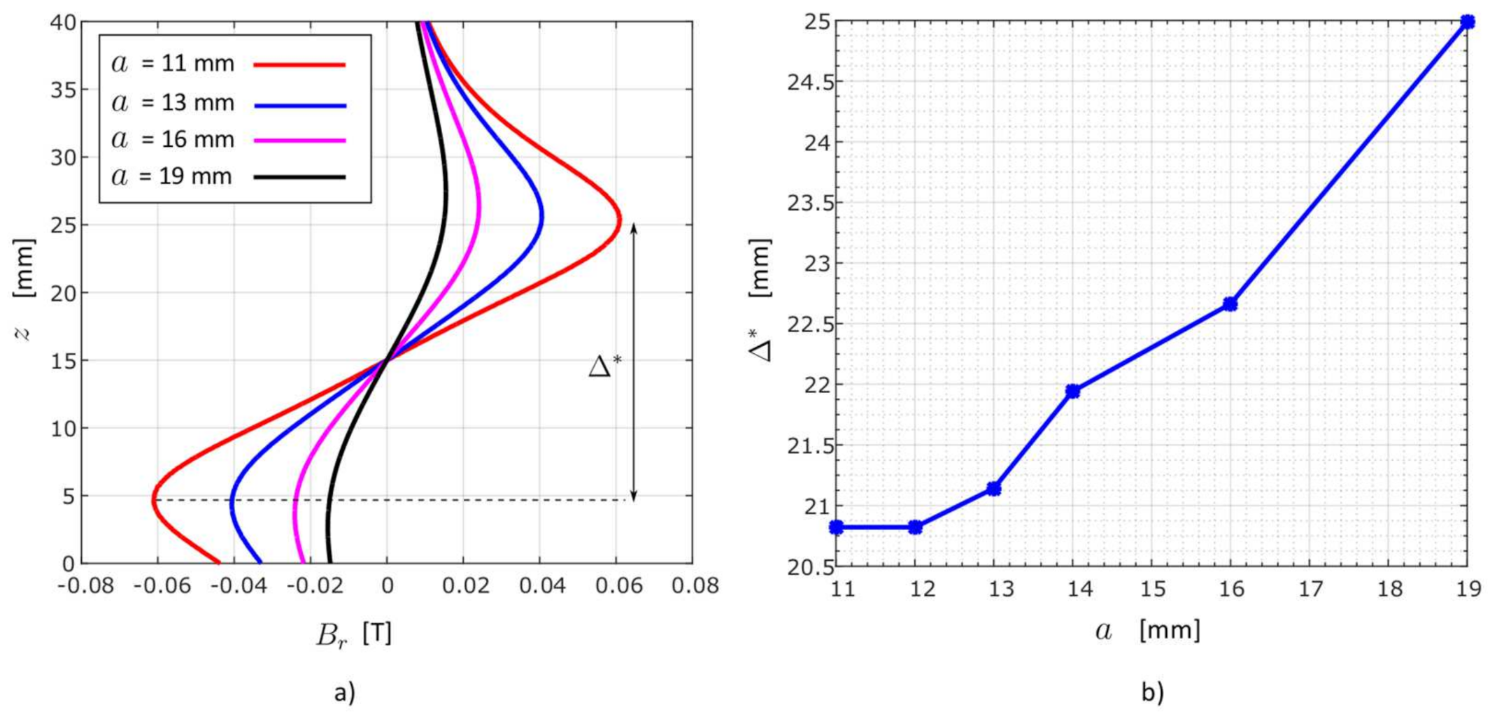
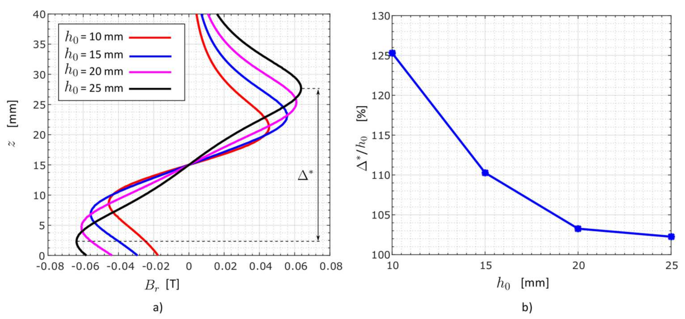
3.3. Parametric Analysis

In order to estimate the technical limits of the presented technique, additional parametric analysis was conducted in the FEMM 4.2 environment. The analysis encompassed a variation of the three crucial parameters, the relative permeability of the ferrofluid μ r , the distance a from the PM’s center to the sensor and the PM’s height, which all affect the magnitude and dispersion of the field in the air. For convenience, the geometry arrangement shown in Figure 9 was adopted to all cases in the analysis. Despite the fact that the levitation height z 0 changed with the magnetic properties of the fluid, the one here was fixed at 5 mm. The goal of the analysis was to appraise the design limits and constraints of the technique.

3.3.1. Variation in the Ferrofluid’s Relative Permeability— μ r

The relative permeability of the ferrofluid was varied in the range from 1 to 4 in the step of 1. For each value of μ r the radial magnetic field component B r was calculated along the line 1 mm distant from the container’s wall, as shown in Figure 10a. The results show that the increase in magnetic permeability of the fluid diminished the magnetic field’s magnitude in the air. The difference between the extreme values of B r , on which basis the estimation of the magnet’s height was brought, increased along with μ r , as shown in Figure 10b. The first parameter’s value μ r = 1 corresponded to the magnetic property of the air.

3.3.2. Variation in the Sensor Distance from the PM Center— a

To see how the magnetic field distribution dispersed with distance a from the magnet’s center, the field was calculated along four vertical lines 11, 13, 16, and 19 mm distant from the PM’s center (Figure 11a). According to the FEM analysis, the sensor should be placed to the container as close as possible to accurately estimate the magnet’s height h 0 . For example, if accuracy within 10% is desired, the distance from the PM to the sensor should not exceed 0.35   h 0 for μ r = 1.31 . The relative permeability used with this virtual experiment was set to unity ( μ r = 1 ).

3.3.3. Variation of the PM’s Height— h 0

The influence of the PM’s height h 0 on the radial field’s peak-to-peak distance Δ * was conducted similarly to the previous cases. The magnetic field was evaluated along the evaluation line, 1 mm distance from the container’s wall ( a = 11 mm). In the simulations, the height of the magnet was changed in four steps: 10 mm, 15 mm, 20 mm, and 25 mm. While the PM’s base remained unchanged, the variation in the PM’s height corresponded to the variation in the PM’s volume to the ferrofluid volume ratio. The relative permeability of ferrofluid in the model was set to μ r = 1 in these simulations. The results plotted in Figure 12 show that much better accuracy in estimation of the PM’s height through the magnetic field was obtained with higher magnets. If the accuracy within 10% is appreciated, the ratio of the PM’s height to its diameter ( h 0 / d 0 ) should not be less than 2.

4. Conclusions

A novel technique in the permanent magnet vertical position detection within the ferrofluid is proposed in the article. Here, the magnet’s center was determined from the radial magnetic field distribution along the vertical line at some distance from the container’s wall. The concept is based on the solenoidal nature of the magnetic field, where the turning point of the radial component corresponds to the center of the magnet. The study on the subject was conducted purely theoretically, where the simulation model was settled in accordance with the experimentally verified physical model [23]. The main goal of the study was the determination of the permanent magnet’s center, for which a numerical evaluation of the magnetic field distribution near the container’s wall was desired. The simulations were conducted for two cases; in the first one, case A, the PM was placed at the bottom of the empty container. In the second simulation setup (case B), the PM was levitating in the ferrofluid-filled container. In both cases, the turning point of the radial field component coincided with the center of the PM.
Furthermore, the results revealed another possibility that could be gathered from the field distribution. Namely, with proper design and experimental setup, the height of the magnet could be achieved with precision under a few percentages. The impact of the ferrofluid’s permeability, PM–sensor distance, and PM’s height on the technique’s accuracy is disclosed in the parametric analysis. In brief, the best results were obtained with ferrofluid with its relative permeability close to unity and with a higher magnet at the nearest PM–sensor distance. For practical design purposes, it is more convenient to express the PM–sensor distance with the magnet’s height, which should not exceed 0.35 h 0 . According to the results shown in Section 3.3.3, an accuracy within 10% was obtained for magnets with the h 0 / d 0 ratio greater than 2. At this point, it should be noted that the presented approach is limited only to simple symmetric magnet shapes such as cylindrical and spherical.
However, the results obtained by the finite element method showed good agreement with the theoretical expectations and open a space for a practical perspective of the proposed approach. Instead of using a single magnetic sensor (i.e., a Hall sensor), an array of sensors can be installed on the container’s wall. With such modification, the magnetic field distribution is scanned instantaneously, and no moving parts are required in the design.
The future work on the subject will be focused on the further improvement and experimental verification of the technique.

Author Contributions

Conceptualization, A.H., M.J., V.G. and M.T.; methodology, M.T.; software, M.T.; validation, M.T. and V.G.; formal analysis, M.T.; investigation, M.T.; resources, M.J.; data curation, M.J.; writing—original draft preparation, M.T.; writing—review and editing, M.T., M.J. and A.H.; visualization, M.T.; supervision, M.J.; project administration, A.H.; funding acquisition, M.J. All authors have read and agreed to the published version of the manuscript.

Funding

This work was supported by the Slovenian Research Agency under grant P2-0114.

Data Availability Statement

All data are presented in the article.

Conflicts of Interest

The authors declare no conflict of interest.

References

  1. Moskowitz, R.; Stahl, P.; Reed, W.R. Inertia Damper Using Ferrofluid. US Patent 4123675, 31 October 1978. [Google Scholar]
  2. Miller, D.L. Magnetic Viscous Damper. US Patent 4200003, 29 April 1980. [Google Scholar]
  3. Kogure, T. Damper Device for a Motor. US Patent 5191811, 9 March 1993. [Google Scholar]
  4. Elsaady, W.; Oyadiji, S.O.; Nasser, A. A one-way coupled numerical magnetic field and CFD simulation of viscoplastic compressible fluids in MR dampers. Int. J. Mech. Sci. 2020, 167, 105265. [Google Scholar] [CrossRef]
  5. Yoon, D.-S.; Par, Y.-J.; Choi, S.-B. An eddy current effect on the response time of a magnetorheological damper: Analysis and experimental validation. Mech. Syst. Sig. Process. 2019, 127, 136–158. [Google Scholar] [CrossRef]
  6. Piso, M.I. Applications of magnetic fluids for inertial sensors. J. Magn. Magn. Mater. 1999, 201, 380–384. [Google Scholar] [CrossRef]
  7. Qian, L.; Li, D.; Yu, J. Study of the Second-Order Levitation Force in the Magnetic Fluid Accelerometer. IEEE Sens. J. 2015, 15, 6805–6810. [Google Scholar] [CrossRef]
  8. Yu, J.; He, X.; Li, D.; Li, W. Effective and Practical Methods to Calculate the Second-Order Buoyancy in Magnetic Fluid Acceleration Sensor. IEEE Sens. J. 2018, 18, 2278–2284. [Google Scholar] [CrossRef]
  9. Bashtovoi, V.G.; Kabachikov, D.N.; Kolobov, A.Y.; Samoylov, V.B.; Vikoulenkov, A.V. Research of the dynamics of a magnetic fluid dynamic absorber. J. Magn. Magn. Mater. 2002, 252, 312–314. [Google Scholar] [CrossRef]
  10. Wang, Z.; Bossis, G.; Volkova, O.; Bashtovoi, K.M. Active Control of Rod Using Magnetic Fluids. J. Intell. Mater. Syst. Struct. 2003, 14, 93–97. [Google Scholar] [CrossRef]
  11. Yang, W. Magnetic levitation force exerted on the cylindrical magnet in a ferrofluid damper. J. Vib. Control 2015, 23, 2345–2354. [Google Scholar] [CrossRef]
  12. Yao, J.; Chang, J.; Li, D.; Yang, X. The dynamics analysis of a ferrofluid shock absorber. J. Magn. Magn. Mater. 2016, 402, 28–33. [Google Scholar] [CrossRef]
  13. Yao, J.; Li, D.; Chen, X.; Huang, C.; Xu, D. Damping performance of a novel ferrofluid dynamic vibration absorber. J. Fluid Struct. 2019, 90, 190–204. [Google Scholar] [CrossRef]
  14. Li, Y.; Li, D. The dynamics analysis of a magnetic fluid shock absorber with different inner surface materials. J. Magn. Magn. Mater 2022, 542, 168473. [Google Scholar] [CrossRef]
  15. Volkova, T.I.; Böhm, V.; Naletova, V.A.; Kaufhold, T.; Becker, F.; Zeidis, I.; Zimmermann, K. A ferrofluid based artificial tactile sensor with magnetic field control. J. Magn. Magn. Mater. 2017, 431, 277–280. [Google Scholar] [CrossRef]
  16. Alberto, N.; Domingues, M.F.; Marques, C.; André, P.; Antunes, P. Optical Fiber Magnetic Field Sensors Based on Magnetic Fluid: A Review. Sensors 2018, 18, 4325. [Google Scholar] [CrossRef] [PubMed] [Green Version]
  17. Ruan, Z.; Pei, L.; Ning, T.; Wang, J.; Wang, J.; Li, J.; Xie, Y.; Zhao, Q.; Zheng, J. Simple structure of tapered FBG filled with magnetic fluid to realize magnetic field sensor. Opt. Fiber Technol. 2021, 67, 102698. [Google Scholar] [CrossRef]
  18. Rosensweig, R.E. Fluidmagnetic Buoyancy. AIAA J. 1966, 4, 1751–1758. [Google Scholar] [CrossRef]
  19. Rosensweig, R.E. Buoyancy and Stable Levitation of a Magnetic Body immersed in a Magnetizable Fluid. Nature 1966, 210, 613–614. [Google Scholar] [CrossRef]
  20. Yang, W.; Li, D.; He, X.; Li, Q. Calculation of magnetic levitation force exerted on the cylindrical magnets immersed in ferrofluid. Int. J. Appl. Electromagn. Mech. 2012, 40, 37–49. [Google Scholar] [CrossRef]
  21. Yang, W.; Wang, P.; Hao, R.; Ma, B. Experimental verification of radial magnetic levitation force on the cylindrical magnets in ferrofluid dampers. J. Magn. Magn. Mater. 2017, 426, 334–339. [Google Scholar] [CrossRef]
  22. He, X.; Li, D.; Yang, W.; Zhang, H. Experimental Study on the Second- Order Buoyancy of Magnetic Fluid. Key Eng. Mater. 2012, 512–515, 1464–1469. [Google Scholar] [CrossRef]
  23. Yu, J.; Chen, J.; Li, D. Experimental error analysis of measuring the magnetic self-levitation force experienced by a permanent magnet suspended in magnetic fluid with a nonmagnetic rod. J. Magn. Magn. Mater. 2019, 469, 323–328. [Google Scholar] [CrossRef]
  24. Yu, J.; Chen, D.; Cai, Z.; Li, D.; Cao, Q.; Qian, L. Research on the magnetic fluid levitation force received by a permanent magnet suspended in magnetic fluid: Consideration a surface instability. J. Magn. Magn. Mater. 2019, 492, 165678. [Google Scholar] [CrossRef]
  25. Wei, Y.; Zhou, H.; Li, D.; Yao, Y.; Chen, Y. Numerical simulation and experimental study on the ferrofluid second-order buoyancy with a free surface. J. Magn. Magn. Mater. 2022, 553, 169013. [Google Scholar] [CrossRef]
  26. Trbušić, M.; Jesenik, M.; Trlep, M.; Hamler, A. Energy Based Calculation of the Second-Order Levitation in Magnetic Fluid. Mathematics 2021, 9, 2507. [Google Scholar] [CrossRef]
  27. Curti, M.; Van Beek, T.A.; Jansen, J.W.; Gysen, B.L.J.; Lomonova, E.A. General Formulation of the Magnetostatic Field and Temperature Distribution in Electrical Machines Using Spectral Element Analysis. IEEE Trans. Magn. 2018, 54, 54–8100809. [Google Scholar] [CrossRef]
  28. Mahariq, I.; Erciyas, A. A spectral element method for the solution of magnetostatic fields. Turk. J. Electr. Eng. Comput. Sci. 2017, 25, 31. Available online: https://journals.tubitak.gov.tr/elektrik/vol25/iss4/31 (accessed on 5 July 2022). [CrossRef] [Green Version]
  29. Koch, S.; De Gersem, H.; Weiland, T. Magnetostatic Formulation With Hybrid Finite-Element, Spectral-Element Discretizations. IEEE Trans. Magn. 2009, 45, 1136–1139. [Google Scholar] [CrossRef]
  30. Mahariq, I.; Abdeljawad, T.; Karar, A.S.; Alboon, S.A.; Kurt, H.; Maslov, A.V. Photonic Nanojets and Whispering Gallery Modes in Smooth and Corrugated Micro-Cylinders under Point-Source Illumination. Photonics 2020, 7, 50. [Google Scholar] [CrossRef]
  31. Kokelj, P. Electromagnetic Structures, 3rd ed.; Založba FE in FRI: Ljubljana, Slovenia, 2003; pp. 147–149. [Google Scholar]
  32. Rosensweig, R.E. Ferrohydrodynamics, 1st ed.; Dover Publications, Inc.: New York, NY, USA, 2014; pp. 150–151. [Google Scholar]
  33. Meeker, D. Finite Element Method Magnetics—User’s Manual. 2007. Available online: www.femm.com (accessed on 31 May 2022).
Figure 1. Illustrative depiction of a key concept in the contactless determination of the PM’s position: (a) the magnetic sensor (Hall sensor) is moving vertically along the evaluation line scanning the magnetic field at points 1–5; (b) vectorial representation of the field at the corresponding points.
Mathematics 10 02499 g001
Figure 2. A permanent magnet and its circular current loop models; (a) PM, (b) multi current loops’ model, and (c) single current loop model.
Mathematics 10 02499 g002
Figure 3. The geometrical arrangement of the current loop accompanying Equations (1) and (2). (a) A thin circular current loop structure and (b) the magnetic field distribution calculated along the z-axis at the distance r = a from the loop origin.
Mathematics 10 02499 g003
Figure 4. PM and the magnetic field distribution along the container’s wall in the air. (a) The container is filled with the air, and (b) the container is filled with the ferrofluid.
Mathematics 10 02499 g004
Figure 5. The geometry pertains to the simulation setup. (a) The PM and container dimensions. (b) The FEM model related to case A in pre-processor mode. (c) The FEM model related to case B in pre-processor mode.
Mathematics 10 02499 g005
Figure 6. The magnetic field distribution for case A encapsulated from the postprocessor mode in FEMM 4.2, and the corresponding values of magnetic field components B r and B z calculated along the evaluation line.
Mathematics 10 02499 g006
Figure 7. The magnetic field distribution for case B encapsulated from the postprocessor mode in FEMM 4.2, and the corresponding values of magnetic field components B r and B z calculated along the evaluation line.
Mathematics 10 02499 g007
Figure 8. The comparison of the numerical results obtained in both cases A and B.
Mathematics 10 02499 g008
Figure 9. The geometrical arrangement used with the parametric analysis.
Mathematics 10 02499 g009
Figure 10. Variation of the relative permeability value. (a) A radial component of the magnetic field B r calculated along the line 1 mm distant from the container. (b) The influence of the ferrofluid’s relative permeability μ r to the field’s peak to peak distance Δ * .
Mathematics 10 02499 g010
Figure 11. Variation of the PM–sensor distance. (a) A radial component of the magnetic field B r calculated along the line 1, 3, 6, and 9 mm remote from the container’s wall. (b) The influence of the PM–sensor distance a to the field’s peak to peak distance Δ * .
Mathematics 10 02499 g011
Figure 12. Variation of the PM’s height h 0 . (a) A radial component of the magnetic field B r calculated along the line 1 mm remote from the container’s wall. (b) The influence of the PM’s height h 0 to the field’s peak-to-peak distance Δ * .
Mathematics 10 02499 g012
Table 1. Values of the parameters used with the FEM models 1.
Permanent Magnet
(PM)
FerrofluidFree Space
(AIR)
materialNdFeB (N38)-Air
ρ (kgm−3)74501377.61.2
μ r 11.311
B r e m (T)1.24--
H c (kAm−1)986.7--
χ i 00.310
Max. mesh size in material (mm)0.250.2510
Max. mesh size at boundary (mm)0.050.05-
Max. mesh size near the eval. line (mm)--0.1
1 Data from ref. [26].
Publisher’s Note: MDPI stays neutral with regard to jurisdictional claims in published maps and institutional affiliations.

