Taylor Series-Based Fuzzy Model Predictive Control for Wheeled Robots

Abstract

In this paper, a new hybrid method for controlling a wheeled robot is introduced. Model predictive control (MPC) is the main controller and a fuzzy controller is used as a compensator. The wheeled robot is a nonlinear, multi-input–multi-output system that requires new and combined methods for precise control. In order to stabilize the system the appropriate control input is set, and at the same time, attention is paid to the reference signal tracking. In the simulation section, several different scenarios are applied and parameter uncertainties and their effects on the controller’s performance are evaluated. The simulation results show the success and efficiency of the proposed method.

1. Introduction

Today, mobile robots are receiving a lot of attention. These robots have a variety of uses and will definitely affect the future of humans. One of the most challenging issues in robotics is their control. System control with non-holonomic constraints is one of the issues that has obtained the attention of many researchers. Among these systems, wheeled mobile robots enjoy a special situation according to their extensive application in the industry. Hence, many studies have been conducted in the field of modeling and controlling these systems [1,2,3,4,5]. Due to the structure of these robots, the wheels roll without slipping and the robots have no speed along the wheels’ axis of rotation. The mentioned restriction is known as a non-holonomic restriction. Mathematically, non-holonomic restrictions are constraints that are not integrable. Considering that these restrictions do not reduce the system degrees of freedom, and these restrictions are also considered alongside the system equations, the existence of these constraints causes increasing complexity in dynamic modeling and the control of these robots. The main challenge in non-holonomic systems is that the number of degrees of freedom that have controllability is less than the total number of system degrees of freedom. Thus, it is considered important to find suitable control inputs for guaranteeing the stability of all state variables.

Many related works have been completed. In the meantime, there is a great significance in the issue of time trajectory tracking with high accuracy in wheeled mobile robots due to the various applications of the robots. For this reason, many studies have been conducted in this field by various methods to investigate tracking and stability, including controller designs based on the Lyapunov method [6], the adaptive control method [7,8], the sliding mode method [9,10,11,12], the feedback linearization method [13], robust control [14,15], the fuzzy method [16,17], the backtracking method [18], a combination of the fuzzy methods of neural networks [19,20], etc. In [21], an optimal proportional-derivative controller based on feedback linearization is designed for tracking the trajectory of a wheeled robot. In other research, the active observer control method based on the Kalman filter for the dynamic control of mobile robots is proposed [22]. Some studies have also used optimal methods, such as the reference [23], in which the optimum controller to the method of time horizon ahead and the predictive control approach based on the model is presented. It should be noted that using numerical calculations methods is not easy for resolving optimization problems; it is difficult to implement them and they have great time delays. The sliding mode control method has been widely used in recent years to control the moving robot, but this method has drawbacks. Among these shortcomings, we can mention the phenomenon of chatting, the lack of proper response in the face of immediate changes, and so on. Experience has shown that if the sliding mode control method is combined with computational intelligence in some way, the above problems can be overcome. The idea of this paper is to use fuzzy control as a complement or compensator to sliding mode control.

In this paper, a novel optimal approach is developed to design a multi-variable nonlinear controller for tracking the trajectory of a wheeled mobile robot, which is then analyzed. This method has been applied by the authors previously to design the controller of an anti-lock braking system with single-input–single-output and multi-input–multi-output mechanisms for tracking wheel slipping [24,25]. The difference between this method and the predictive control method based on the used model in previous works is that, in general, the common predictive control method in each control step requires solving the optimization problem simultaneously and numerically and for this reason it has delays, and so it is not appropriate for implementation. However, the proposed control method in this paper utilizes control–analysis laws with no mentioned problems. The basis of this method is to predict the response of the nonlinear model of the robot. In this way, the nonlinear response of the robot is predicted by Taylor series expansion at first, and then the control law is obtained by minimizing the differences in desired responses and predicted ones. On the other hand, according to the main challenge in non-holonomic systems mentioned before, the capability of this method can be named in finding suitable control inputs for guaranteeing the stability of all desired state variables. After designing the controller, the analysis of the tracking error is analytically investigated and the effect of the predicted time parameter as a control-free parameter is examined, and it will be demonstrated that the control laws lead to feedback linearization. In order to indicate the efficiency of the designed control system, the required simulations on the robot model with three degrees of freedom with various maneuvers are conducted. The results of the analysis and simulations denote the suitable performance of the proposed control system in achieving the desired goals.

The novelty of this paper is as follows:

• The MPC design for the robot system is based on the Taylor series expansion;
• Using the fuzzy control system as compensation for the main control system when the model’s uncertainty is high.

2. Statement of the Problem

The general structure of a wheeled mobile robot composed of two mobile wheels located on one axis is shown in Figure 1. The wheels have the same radius r and are located at a distance of l. Both wheels move to shift and orient the robot independently by two actuators (two DC motors). According to Figure 1, the robot in the two-dimensional plane composed of three degrees of freedom includes two translational motions and one rotational motion. Thus, (x,y) is the position of the axis center on which the wheels are located and θ denotes the angle of robot placement.

Due to the fact that the robot has no velocity along the rotation axis of wheels, we conclude:

$$\left[\begin{array}{c}-\sin \theta \cos \theta \end{array}\right]\left[\begin{array}{c}\dot{x}\\ \dot{y}\end{array}\right]=0$$

(1)

The above constraint equation is not integrable and thus it is known as a non-holonomic constraint. Moreover, the governing equations based on the first-order kinematic model of the robot are:

$$\dot{q}=\left[\begin{array}{c}\dot{x}\\ \dot{y}\\ \dot{\theta }\end{array}\right]=\left[\begin{array}{cc}\cos \theta & 0\\ \sin \theta & 0\\ 0& 1\end{array}\right]\left[\begin{array}{c}v\\ \omega \end{array}\right]$$

(2)

Thus, $q^T=\left[\begin{array}{c}x y \theta \end{array}\right]$ is the generalized coordinate vector, v is translational velocity, and $\omega$ is the angular velocity of the robot. In the control system, this will be used from two positions, $q_c^T=\left[x_c y_c {\theta }_c\right]$ and $q_r^T=\left[\begin{array}{c}{x}_r y_r {\theta }_r\end{array}\right]$, where the first is related to the position or reference trajectory of the robot that must be tracked by the controller.

According to Figure 2 and considering the reference coordinate system $x-y$ and the relative coordinate system $x^{\prime }-y^{\prime }$ to center of $\left(x_c-y_c\right)$ and in the direction ${\theta }_c$, the position error $e^T=\left[\begin{array}{c}{e}_x e_y e_{\theta }\end{array}\right]$ can be defined by the following:

$$\left[\begin{array}{c}{e}_x\\ e_y\\ e_{\theta }\end{array}\right]=\left[\begin{array}{ccc}\cos {\theta }_c& \sin {\theta }_c& 0\\ -\sin {\theta }_c& \cos {\theta }_c& 0\\ 0& 0& 1\end{array}\right]\left(q_r-q_c\right)$$

(3)

By using relationship (2), we have:

$${\dot{x}}_r\sin {\theta }_r={\dot{y}}_r\cos {\theta }_r$$

(4)

Now, by differentiating Equation (3) using relationship (4) and some mathematical calculations, it can be obtained that the error model is as follows [26]:

$$\left[\begin{array}{c}{\dot{e}}_x\\ {\dot{e}}_y\\ {\dot{e}}_{\theta }\end{array}\right]=\left[\begin{array}{cc}\cos e_{\theta }& 0\\ \sin e_{\theta }& 0\\ 0& 1\end{array}\right]\left[\begin{array}{c}{v}_r\\ {\omega }_r\end{array}\right]+\left[\begin{array}{cc}-1& e_y\\ 0& -e_x\\ 0& -1\end{array}\right]\left[\begin{array}{c}v\\ \omega \end{array}\right]$$

(5)

It should be noted that, in all relationships, the index r is related to the reference model.

3. Control System Design

By writing the Equation (5) in the form of the following state space, we have:

$$\{\begin{array}{c}{\dot{x}}_1=v_r\cos x_3-u_1+x_2{u}_2\\ {\dot{x}}_2=v_r\sin x_3-x_1{u}_2\\ {\dot{x}}_3={\omega }_r-u_2\end{array}$$

(6)

where, $x^T=\left[\begin{array}{c}{x}_1 x_2 x_3\end{array}\right]=\left[\begin{array}{c}{e}_x e_y e_{\theta }\end{array}\right]$ is the state variable vector and $u^T=\left|u_1 u_2\right|=\left[\begin{array}{c}v \omega \end{array}\right]$ is the control input vector. The purpose is to design a controller with two inputs for the system with Equation (6), so that by tracking the reference trajectory the tracking error $e^T=\left[e_x e_y e_{\theta }\right]$ equals zero and, in other words, the stability of the mentioned system is guaranteed. Here, it will be used in the predictive nonlinear control method based on optimization. In general, in this method, firstly, the intended system outputs are predicted by the Taylor series expansion and then by minimizing the performance function, which is defined based on the predicted errors; the control laws are then optimally and analytically obtained. In addition to the mentioned advantages of this method, the capability for stabilizing a nonlinear system by selecting suitable outputs can also be mentioned. By selecting the following outputs, we have:

$$\{\begin{array}{c}{y}_1=x_1-x_2\mathrm{sgn}\left({\omega }_r\right)\\ y_2=x_3\end{array}$$

(7)

where $\sin (.)$ is the sign function. In the section analyzing and evaluating the control laws, it will be shown that selecting the above outputs leads to the feedback linearization of the system’s input–output and consequent stabilization. Now, for developing the nonlinear control laws, a performance index is written in such a way that penalizes the tracking errors at the next instant, as follows:

$$J\left(u_1,u_2\right)=\frac{1}{2}{\sum }_{i=1}^2{e}_i^2(t+h)i=1,2$$

(8)

where h is the predictive time and a positive real number and the tracking errors are e_i. In this equation, Yi is the output of the system and the Yd is the desired output of the system.

$$e_i\left(t+h\right)=y_i\left(t+h\right)-y_{di}\left(t+h\right)i=1,2$$

(9)

Since it is supposed that there is no restriction on the control input for achieving the complete tracking, the performance index (8) does not involve the weight of the control input; in other words, the design based on the control is inexpensive. On the other hand, the significance of tracking errors is supposed to be the same, and so it is considered to have the same weight on the errors. Now, in order to develop performance index (8) as a function of control input, it is necessary that the system outputs are predicted for the next time interval by the Taylor series expansion. First, $y_i\left(t+h\right)$ is extended by the Taylor series in q th order in the time t as follows:

$$\begin{array}{c}{y}_i\left(t+h\right)=y_i\left(t\right)+h{\dot{y}}_i\left(t\right)+\frac{h^2}{2!}{\ddot{y}}_i\left(t\right)+\\ \cdots +\frac{h^q}{q!}{y}_i^{\left(q\right)}\left(t\right)i=1,2\end{array}$$

(10)

In the following, the main issue is selecting the order of expansion q for system outputs so that it is proportional to the design goals of the controller based on prediction. Usually, the expansion order that denotes the highest derivation order of the used output in prediction is bound to add to the relative degree of the nonlinear system and the selected control order [27]. The relative degree of the dynamic equations of the nonlinear system is acquirable and it is equal to the lowest order of output derivation in which the control input appears in equations as explicit for the first time [28]. According to the equations of system (6), both system outputs to both inputs have a relative degree 1, q = 1. On the other hand, to reach the low control energy and to prevent the complexity of control law, here, the control order is bounded at the least possible, i.e., zero. This selection, i.e., control order 0, causes the control energy to remain constant in a predictive time interval and does not appear as a control input derivation in the prediction of the output.

$$\frac{d}{d\tau }u\left(t+\tau \right)=0\mathrm{for}\tau \in \left[0,h\right]$$

(11)

Selecting the control order 0 for nonlinear systems with low relative degrees is appropriate [29]. Commonly, the control order is set as the free parameter, and it is determined by the designer proportional to the control system characteristics and control energy restrictions.

Thus, according to the above reasons, the first-order series is proportional to the relative degree of the system and is adequate for the expansion of system outputs.

$$y_i\left(t+h\right)=y_i\left(t\right)+h{\dot{y}}_i\left(t\right)i=1,2$$

(12)

By placing Equation (6) into (12) and using the selected outputs, we have:

$$\begin{array}{c}{y}_1\left(t+h\right)=y_1+h\left({\dot{x}}_1-{\dot{x}}_2\right)\\ \hspace{1em}\hspace{1em}\hspace{1em}\hspace{1em} =x_1-x_2\mathrm{sgn}\left({\omega }_r\right)+h(x_2{u}_2-u_1+\\ \hspace{1em}\hspace{1em}\hspace{1em}\hspace{1em}\hspace{1em} v_r\cos x_3+x_1{u}_2-v_r\sin x_3)\\ y_2\left(t+h\right)=y_2+h{\dot{x}}_3\\ \hspace{1em}\hspace{1em}\hspace{1em}\hspace{1em} =x_3+h\left({\omega }_r-u_2\right)\end{array}$$

(13)

Now, by placing Equation (13) in (8) and given that the desirable values of the outputs are equal to zero, the expanded performance index is obtained as a function of the control inputs. By applying the optimization condition, we have:

$$\begin{array}{c}\frac{\partial J}{\partial u_1}=0\Rightarrow A_{11}{u}_1+A_{12}{u}_2+B_1=0\\ \frac{\partial J}{\partial u_2}=0\Rightarrow A_{21}{u}_1+A_{22}{u}_2+B_2=0\end{array}$$

(14)

Therefore, the control laws are calculated as follows:

$$u_1=-\frac{1}{A_{11}}\left(A_{12}{u}_2+B_1\right)$$

(15)

$$u_2=\frac{B_2{A}_{11}-B_1{A}_{12}}{A_{12}{}^2-A_{11}{A}_{22}}$$

(16)

Thus,

$$\begin{array}{cc}\hfill A_{11}=& -h,A_{12}=h\left(x_1+x_{2}sgn\left({\omega }_r\right)\right),\hfill \\ \hfill B_1=& x_1-x_{2}sgn({\dot{\varphi }}_r)+h{v}_r\left(cos{x}_3-sin{x}_{3}sgn\left({\omega }_r\right)\right),\hfill \\ \hfill A_{21}=& -h\left(x_1+x_{2}sgn\left({\omega }_r\right)\right),\hfill \\ \hfill A_{22}=& h\left(1+{\left(x_1+x_{2}sgn\left({\omega }_r\right)\right)}^2\right),\hfill \\ \hfill B_2=& -\left(x_3+h{\omega }_r\right)+\left(x_2+x_{1}sgn\left({\omega }_r\right)\right)\left(x_1-x_{2}sgn\left({\omega }_r\right)\right.\hfill \\ \hfill & \left.+h{v}_r\left(cos{x}_3-sin{x}_{3}sgn\left({\omega }_r\right)\right)\right)\hfill \end{array}$$

(17)

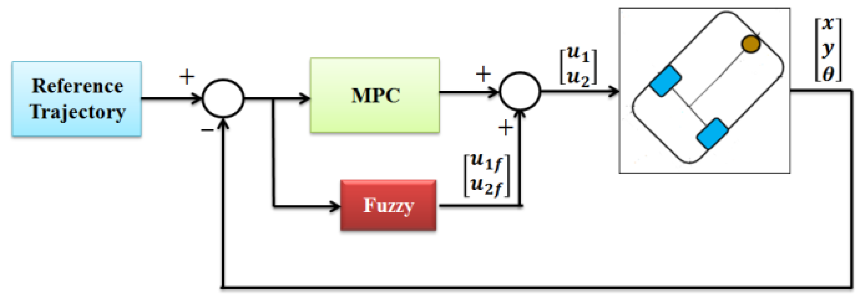
The expanded form of the control law, by placing relationship (17) in (15) and (16), with some simplifications, is computable as follows:

$$\begin{array}{c}{u}_1=\frac{1}{h}(x_1-x_2\mathrm{sgn}\left({\omega }_r\right)+\left(x_2+x_1\mathrm{sgn}\left({\omega }_r\right)\right)\left(x_3+h{\omega }_r\right)\\ \hspace{1em}\hspace{1em}+h{v}_r\left(\cos x_3-\sin x_3\mathrm{sgn}\left({\omega }_r\right)\right))+u_{1f}\end{array}$$

(18)

$$u_2=\frac{1}{h}\left(x_3+h{\omega }_r\right)+u_{2f}$$

(19)

The fuzzy compensator signals are $u_{1f}$ and $u_{2f}$. The above feedback control laws that have close form minimize the performance of function (8). Here, the control inputs of linear velocity and angular velocity are calculated. The required torques applied to the wheels for generating the mentioned inputs of the dynamic model of the robot must be calculated. In the next section, the obtained control laws are analyzed and evaluated. The block diagram of the proposed control method is shown in Figure 3.

Analyzing and Evaluating the Control Laws

In this section, the main specifications of control laws (18) and (19), and also the significance of the free parameter of predictive time h in the control laws, will be examined. By differentiating the first output of relationship (7) by supposing ${\omega }_r\ne 0$ and placing the system Equation (6) into it, we have:

$$\begin{array}{c}{\dot{y}}_1={\dot{x}}_1-{\dot{x}}_2\mathrm{sgn}\left({\omega }_r\right)\\ \hspace{1em} =-u_1+u_2\left(x_2+x_1\mathrm{sgn}\left({\omega }_r\right)\right)+\\ \hspace{1em}\hspace{1em}{v}_r\left(\cos x_3-\sin x_3\mathrm{sgn}\left({\omega }_r\right)\right)\end{array}$$

(20)

Placing control laws (18) and (19) in relationship (20) leads to:

$${\dot{y}}_1+\frac{1}{h}{y}_1=0$$

(21)

Likewise, we have this for the second output:

$${\dot{y}}_2+\frac{1}{h}{y}_2=0$$

(22)

It is obvious that the dynamic of errors (21) and (22) are linear and time-independent. It can be seen that the control laws lead to the special state of linearization of the input–output. Thus, the closed loop system is linear and, when h > 0, is exponentially stable, and by minimizing the predictive time h, response speed can be increased. In this case, we have:

$$\mathrm{if}t\to \infty ,\Rightarrow \{\begin{array}{c}{y}_1\to 0\Rightarrow x_1\to x_2\mathrm{sgn}\left({\omega }_r\right)\\ y_2\to 0\Rightarrow x_3\to 0\end{array}$$

(23)

Now, by placing relationship (23) and the control laws (18) and (19) into the first two equations of Equation (6), we have:

$${\dot{x}}_1+{\omega }_r\mathrm{sgn}\left({\omega }_r\right)x_1=0$$

(24)

$${\dot{x}}_2+{\omega }_r\mathrm{sgn}\left({\omega }_r\right)x_2=0$$

(25)

Considering that ${\omega }_r\ne 0$, Equations (24) and (25) are exponentially stable and we have:

$$\mathrm{if}t\to \infty \Rightarrow \{\begin{array}{c}{x}_1\to 0\\ x_2\to 0\end{array}$$

(26)

Thus, considering Equations (22), (24) and (25), it can be concluded that the proposed control system with control laws (18) and (19) makes the tracking error $e^T=\left[e_x{e}_y{e}_{\theta }\right]$ equal to zero. In the next section, in order to indicate the performance of the designed control system faced with various maneuvers, the performed simulation results will be investigated.

4. Simulation Results

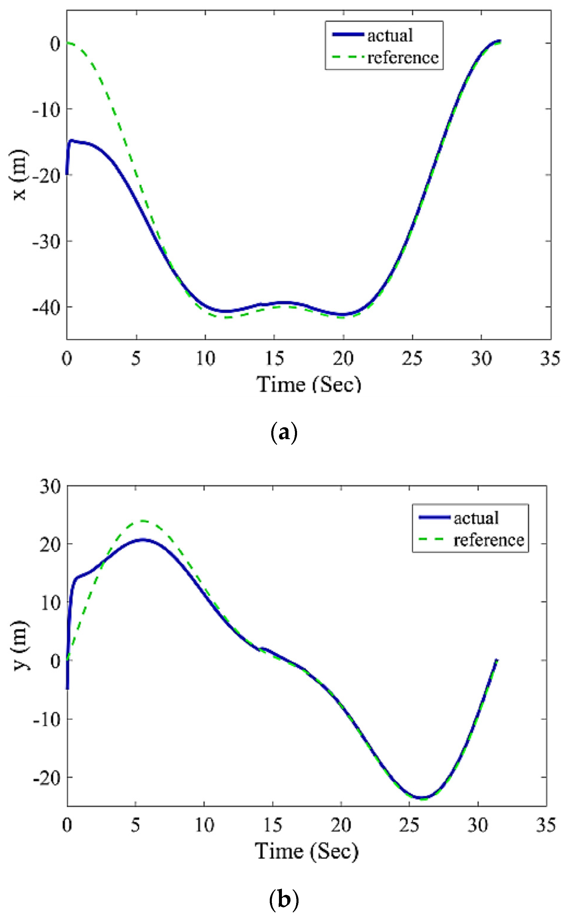
To denote the performance of the control system, the required simulations on a kinematic model of a wheeled mobile robot with three degrees of freedom were performed in MATLAB software, version 2015-a. To investigate the controller performance in real conditions, we applied white noise to the state variables of the system. In the first maneuver, the purpose was to achieve a tracking reference model with the following equations:

$$\begin{array}{c}{x}_r=3 \sin t\\ y_r=3 \sin \left(2t\right)\end{array}$$

(27)

According to relationship (27), the first position of the reference trajectory is $x_r\left(0\right)={(0,0,1.1071)}^T$. The real first position of the robot $x\left(0\right)={(0,2,\pi /4)}^T$ is also considered. In Figure 4, the time change of the robot’s position variables (x,y) is shown.

As it can be seen from this figure, the time responses of the robot’s positions were able to quickly reach the responses of the reference model. By comparing the robot trajectory to the reference trajectory in Figure 5, it can be found that the designed controller was able to track the desirable trajectories with high accuracy.

Moreover, in Figure 6, the tracking errors of the robot’s longitudinal position (ex,ey) and the tracking error of the angular position of the robot e_θ, are shown. It is seen that, in any case, the initial error quickly reached 0.

In order to indicate the effect of control parameter h on the performance of the control system, Figure 7 simulates the tracking error of the robot’s angular position for different values of predictive time. It can be seen that, by reducing the value of predictive time h, the tracking error decreased and the response speed increased. It should be noted that reducing predictive time causes an increase in control energy at the start of the maneuver. This is because the control energy is inversely related to the predicted time corresponding to the control laws (18) and (19). Thus, we can compromise between the tracking error and the control energy by adjusting the control parameter h.

In the second maneuver, the purpose is to track the reference model by the following equations:

$$\begin{array}{c}{x}_r=\left(20+15 \cos \left(0.2t\right)\cos \left(0.2t\right)-35\right)\\ y_r=\left(20+15 \cos \left(0.2t\right)\sin \left(0.2t\right)\right)\end{array}$$

(28)

Considering relationship (28), the initial position of the reference trajectory is $x_r\left(0\right)={(0,0,\pi /2)}^T$. The real initial position of the robot is considered as $x\left(0\right)={(-20,-5,\pi /3)}^T$. To observe the brevity, it is selected and plotted in only a few diagrams in this maneuver. Figure 8 and Figure 9 show the comparison of the time responses of the robot’s position and the robot’s trajectory in the plane x-y with the reference responses.

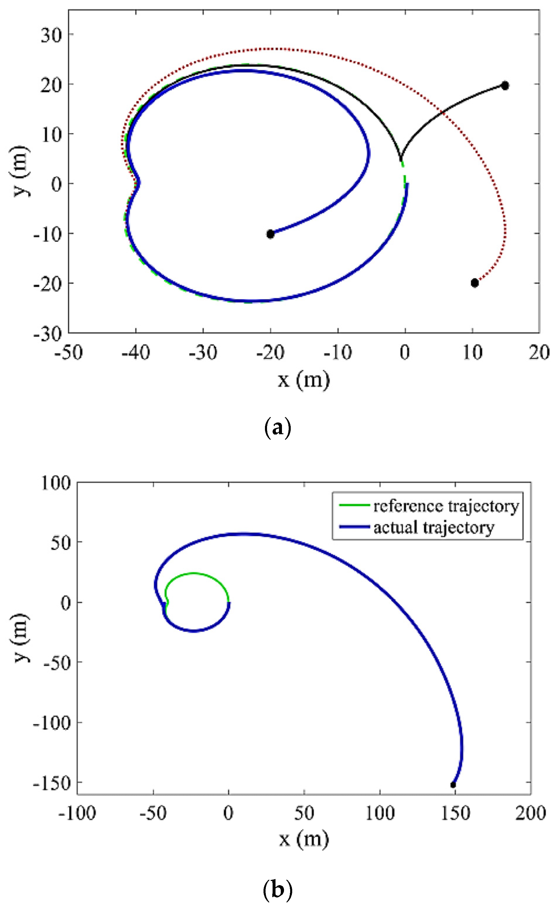
In Figure 10, the tracking errors of the robot’s longitudinal position (ex,ey) and the tracking error of the robot’s angular position e_θ, are shown. It can be seen that, in this maneuver, the responses also had a great adaptation with the reference responses. At the end, in order to indicate the performance of the control system in various initial conditions, Figure 11 is simulated. In Figure 11a, it can be seen that, for various initial conditions, the robot was well able to track the desired reference trajectory. To indicate the performance of the control system, Figure 11b is simulated for the initial conditions far from the reference trajectory. It can be seen that the initial conditions being so far from the reference trajectory affects the time and the quality of reaching the reference trajectory, but the reference trajectory is tracked with acceptable accuracy.

As can be seen from the simulation results, the combined fuzzy control system and the MPC had a good performance and can be further considered in the future.

In order to show the effectiveness of the proposed method, a comparison has been made with the methods presented in [25,27]. The comparison criterion is the root mean square error or RMSE.

The RMSE criterion is very common and important in control engineering articles. As can be seen in

Table 1. Comparison of the proposed method with two other methods.

	Proposed Method	Method of [25]	Method of [27]
First maneuver	0.0011	0.0018	0.0025
Second maneuver	0.0096	0.0108	0.0110

, based on this criterion, the proposed method performed much better than the other two methods. Definitely, the reason for this better performance was the use of the compensating fuzzy controller next to the main controller. In places where the error was high, the fuzzy control system was activated and produced a relatively large signal so that the robot immediately approached the path.

5. Conclusions

In the future, mobile robots will definitely be used in abundance. One of the most challenging issues with these systems is the precise control of them. In this paper, a predictive control method for designing multi-input–multi-output nonlinear controllers in analytical and optimum forms is developed to track the reference trajectory of a wheeled mobile robot. A fuzzy control system was used to compensate the MPC. In addition, by selecting the suitable outputs, the appropriate control inputs were extracted for the stabilization of the system. The dynamic of the tracking error of the proposed controller was extracted and the stabilization of all states of the system was investigated. Finally, the simulation results in the various maneuvers denoted the proper performance of the proposed control system in reaching the desired purposes.