Leveraging Geographically Distributed Data for Influenza and SARS-CoV-2 Non-Parametric Forecasting

Abstract

The evolution of some epidemics, such as influenza, demonstrates common patterns both in different regions and from year to year. On the contrary, epidemics such as the novel COVID-19 show quite heterogeneous dynamics and are extremely susceptible to the measures taken to mitigate their spread. In this paper, we propose empirical dynamic modeling to predict the evolution of influenza in Spain’s regions. It is a non-parametric method that looks into the past for coincidences with the present to make the forecasts. Here, we extend the method to predict the evolution of other epidemics at any other starting territory and we also test this procedure with Spanish COVID-19 data. We finally build influenza and COVID-19 networks to check possible coincidences in the geographical distribution of both diseases. With this, we grasp the uniqueness of the geographical dynamics of COVID-19.

1. Introduction

Influenza (or flu) is an infectious respiratory disease caused by the influenza virus. It results in an estimated 250,000 to 650,000 deaths annually [1]. Until 2020, influenza epidemics demonstrated a seasonal recurrence (Figure 1a), with a yearly pattern of exponential growth of infections, a marked peak, and a similarly prompt decay of new cases (Figure 1b). The width and magnitude of each outbreak varied moderately across years. These overall regularities [2] allowed a moderate success of different modeling approaches in forecasting outbreak magnitude and duration [3,4,5,6].

In late 2019, the emergence of the COVID-19 (the infectious respiratory disease caused by the SARS-CoV-2 virus) global pandemics disrupted the seasonal influenza pattern [7]. The fast spread and severity of the disease led to the enforcement of strong distancing measures around the globe, which halted the propagation of other, less aggressive respiratory viruses such as influenzas [8]. Contrary to the regularities observed in flu epidemics, COVID-19 data is very erratic. On the one hand, we do not know yet whether it will become a stationary disease—with patterns of infection growth and decay similar to those of flu. If that were the case eventually, we have not observed the new epidemics for a sufficiently long time yet as to infer repeated trends. On the other hand, while influenza is dealt with casually, the countermeasures to tackle COVID-19 have disrupted its natural cycle. When these countermeasures were relaxed, new outbreaks emerged. This resulted in an irregular train of waves that often overlapped in time. As measures were dictated by an array of authorities (from local to supra-national), these waves differed wildly across regions—even within a same country (Figure 1c). Some biological aspects of SARS-CoV-2 contributed to the disarray: it presents a long incubation period [9] during which an infected person does not show symptoms; a large fraction of people suffer an asymptomatic version of the disease, but they can propagate the virus [10]; and, also, large outbreaks have been attributed to single super-spreaders who infected up to hundreds of people during a single event [11]. Under such conditions, tracking the exact timing of each infection is difficult—which resulted in unreliable epidemiological time series.

The very mathematical nature of epidemic dynamics also hinders its forecasting [12]. A popular approach to this problem are compartmental models. In them, a population is coarse-grained into broad classes (e.g., Susceptible, Infected, and Recovered) and simple rules are established to regulate the flows between compartments. Typically, Infected people move into the Recovered class at a given rate, while they infect Susceptible individuals (moving them to the Infected compartment) with some probability. These rates and probabilities can be empirical model parameters inferred from the data. Such simple models can correctly capture broad qualitative aspects—e.g., a phase of exponential growth or the existence of herd-immunity thresholds. However, these models are notably bad at forecasting real-life scenarios. On top of all the troubles affecting data quality mentioned above, the phase of exponential growth in epidemic dynamics constitutes an important limiting factor. As it happens in deterministic chaos [13], small errors or uncertainties in the data are magnified exponentially by the epidemic dynamics themselves. Unlike chaotic systems, epidemic peaks can be fairly stereotypical; but the effect of exponentially magnified errors is enough to prevent a systematic and precise forecast of an outbreak’s magnitude and duration [12]. This exponential factor in epidemic dynamics results in broad ranges or parameters that can fit correctly past data, but that are compatible with wildly diverging future behaviors.

In this framework, we have turned our attention to Empirical Dynamic Modeling (EDM) [14], a form of non-parametric modeling that looks at past examples of how a dynamical process (e.g., an epidemic) looked like, and uses them to forecast how it might unfold. Traditional EDM applications take a specific historic time-series (e.g., epidemic data of influenza in a French region [15]), then look at more recent data (say, the last 5 weeks of influenza cases in that same region) and find instances of the past series that resemble the new data. The known progress of the closest historical matches is used as an estimate for the evolution of the current situation. This avoids fitting empirical data to highly sensitive exponential dynamics that magnify small errors. Instead, it relies on bounded, repeated trends of a same kind.

Because of the issues around SARS-CoV-2 data outlined above, EDM seems still an unfit technique for the ongoing pandemic. The strong regularities observed in influenza mitigate some of these problems, making it an excellent test-bench for this approach. In an attempt to improve forecasting for the current pandemics, we expanded the classical functioning of EDM to leverage geographically distributed data. Instead of using a single historic time series to predict what might happen in a specific region, we studied a set of areas on which epidemics unfolded simultaneously, and allowed historical series from each-other to serve as examples of how the dynamics might progress. We first used influenza data from different Spanish regions to study a controlled scenario of known regularity. Through this controlled case, we quantified how much of an improvement our approach is with respect to earlier applications of EDM that did not leverage similar dynamics in geographically distributed data. We briefly explore the more difficult case of SARS-CoV-2, in which data remains scarce and heterogeneity across regions is more pronounced. Our approach is moderately successful in capturing some features of the epidemics in different Spanish regions, while it fails in some important aspects. We propose that pooling geographically distributed data might speed up the gathering of recurring patterns, thus enhancing forecasting methods (beyond EDM) if COVID-19 becomes a seasonal disease. Finally, we turned EDM on its head to infer relationships between epidemic dynamics across different Spanish regions and over time. Since EDM uses past examples to forecast future dynamics, we quantified how often dynamical patterns from a region and year served as an estimate for each other’s unfolding. Thus, we derive networks that illustrate epidemiological patterns across regions and correlations between flu strains from different years. These might offer relevant information to track which are the closest patterns that new epidemics follow.

2. Materials and Methods

2.1. Data and Data Preprocessing

We obtained time series of influenza cases from the Spanish National Center for Epidemiology (Instituto de Salud Carlos III). Out of 19 Spanish regions, we gathered data for 17 (which include 15 autonomous communities and the autonomous cities of Ceuta and Melilla). Data spans from 2000 to 2020, with some regions starting off at different times (as summarized in

Table A1. Length (number of data points) of each series. It spans from early 2000s to the beginning of 2020, but some series miss data from the beginning or the end. Their span is exhibited in brackets (beginning year—last year). Influenza data is weekly and only contains data from September to June. COVID-19 data is daily, from the beginning of the pandemic until 19 April 2021.

	Influenza	COVID-19
Andalusia (AN)	679 (00-20)	429
Aragon (AR)	615 (00-18)	421
Asturias (AS)	549 (04-20)	412
Balearic Islands (IB)	672 (00-20)	416
Basque Country (PV)	661 (00-20)	429
Canary Islands (CN)	582 (03-20)	419
Cantabria (CB)	539 (05-20)	415
Castile and León (CL)	681 (00-20)	423
Castile-La Mancha (CM)	681 (00-20)	416
Catalonia (CT)	495 (05-20)	442
Ceuta (CE)	489 (05-20)	402
Community of Madrid (MD)	661 (00-20)	457
Extremadura (EX)	582 (03-20)	416
Galicia (GA)	-	420
La Rioja (RI)	549 (04-20)	417
Melilla (ML)	356 (09-20)	405
Navarre (NC)	549 (04-20)	418
Region of Murcia (MC)	-	415
Valencian Community (VC)	679 (00-20)	429

). Each time series starts at week 40 of a year and ends on week 20 of the next year—thus skipping the warm season in which influenza is uncommon. Raw data consists of weekly incidence per 100,000 inhabitants. This was smoothed with a 3-week moving average to mitigate sampling effects.

We obtained COVID-19 time series from the same Instituto de Salud Carlos III. This data spans from the beginning of the epidemic to 19 April 2021. Raw data consists of the cumulative cases of COVID-19 in each Spanish region (all the Autonomous Communities, and the independent cities Ceuta and Melilla). We smooth the data with a 7-days moving average to mitigate sampling effects. From here, we derive daily incidence for each region and report it as number of cases per 100,000 inhabitants.

Let us denote the time series of weekly (for flu) or daily (for COVID-19) new cases as $x\left(t\right)$, where $t\in \{T_0,\dots ,T_{end}\}$ is a discrete index in units of weeks or days, respectively. Given data up to some time t, our task is to attempt a forecast for $x(t^{\prime }>t)$. Following the literature on EDM (our tool of choice), we will work with the discrete derivative of $x\left(t\right)$:

$$\begin{array}{ccc}\hfill \Delta x\left(t\right)& \equiv & x\left(t\right)-x(t-\Delta t).\hfill \end{array}$$

(1)

We will base our forecast on this variable instead of on $x\left(t\right)$. This choice removes the effect of short-term linear auto-correlations [14].

2.2. Empirical Dynamic Modeling

Two approaches to forecasting stand out in the literature. On the one hand, modeling based on agents or equations try to capture the underlying causal processes behind a phenomenon (in our case, epidemic dynamics). Such causality is encoded by parameters—e.g., the likelihood that a contagious person infects someone else, or that he/she recovers from the disease. This approach allows us to understand a process and to test hypotheses to control it, but it is very sensitive to the array of problems discussed in the introduction. Non-parametric modeling, on the other hand, foregoes any attempt at understanding the mechanisms behind a phenomenon. These methods are more pragmatic—blindly seeking to extract as much useful information as possible to predict future scenarios. Little care is put on distilling this information into simple operating principles.

Empirical Dynamic Modeling (EDM) [14] is a non-parametric forecasting technique. EDM builds a library of dynamical patterns observed in the past history of a time series. Then, an ongoing situation is matched to examples from this library. The evolution of the matching examples becomes an estimator of how the current situation might progress. This method has been used in epidemiology under alternative names, such as the “Method of Analogues” [15].

To the best of our knowledge, all applications of EDM base their forecast for an ongoing time series on examples drawn from its own past history. This does not help much for the current SARS-CoV-2 global pandemics, for which at most one year of very irregular data exists. However, the epidemics have unfolded simultaneously throughout the world, effectively generating parallel samples of the same process. Can we leverage this geographically distributed information? To do so, we expand EDM’s library of examples not only to the past of some ongoing dynamics, but to ongoing processes across different regions.

Let there be a short time series:

$$\begin{array}{ccc}\hfill Y& \equiv & \left[y(t-n_L+1),y(t-n_L+2),\dots ,y\left(t\right)\right].\hfill \end{array}$$

(2)

This usually consists of the last $n_L$ data points of an ongoing process, of which we wish to forecast the immediate future. The length of this short series ($n_L$) will be chosen as explained below. Additionally, let there be a set of longer time series:

$$\begin{array}{ccc}\hfill {\tilde{Y}}^r& \equiv & \left[{\tilde{y}}^r\left(T_0^r\right),\dots ,{\tilde{y}}^r\left(T_{end}^r\right)\right];\hfill \end{array}$$

(3)

where the superscript r labels all available regions, and each corresponding series runs between times $T_0^r$ and $T_{end}^r$ (which might differ between regions). Let us call $\tilde{Y}\equiv \left\{{\tilde{Y}}^r\right\}$ to the collection of all such series from all regions. $\tilde{Y}$ constitutes our library of dynamic patterns, upon which we will base our forecast for the future of Y.

To build this forecast, we first search for dynamical patterns in $\tilde{Y}$ that resemble Y. We compute the Euclidean distance between Y and each stretch of length $n_L$ within $\tilde{Y}$:

$$\begin{array}{ccc}\hfill d_{t^{\prime }}^r& =& \sqrt{\sum _{i=1}^{n_L}{\left(y(t-n_L+i)-{\tilde{y}}^r(t^{\prime }-n_L+i)\right)}^2},\hfill \end{array}$$

(4)

where we have selected each suitable stretch from region r and labeled it with its ending time $t^{\prime }$. Note that both Y and each stretch of length $n_L$ within the library are a point in an $n_L$-dimensional space. Equation (4) tells us how close to Y each point in the library is in this abstract space. Of all the examples available, we select the $n_B$ closest neighbors to Y. In this paper (and following suit with EDM literature [14]), we take

$$\begin{array}{c}\hfill n_B\equiv n_L+1.\end{array}$$

(5)

We denote the selected neighbors as $\{{\widehat{Y}}_i;i=1,\dots ,n_B\}$. Alongside these examples we store h time steps into their future, such that:

$$\begin{array}{ccc}\hfill {\widehat{Y}}_i& \equiv & \left\{{\widehat{y}}_i(t_i^{\prime }-n_L+1),\dots ,{\widehat{y}}_i\left(t_i^{\prime }\right),{\widehat{y}}_i(t_i^{\prime }+1),\dots ,{\widehat{y}}_i(t_i^{\prime }+h)\right\}.\hfill \end{array}$$

(6)

Note that the index $t_i^{\prime }$ labels time differently within each selected example. We estimate the future h time steps ahead of the last point in Y as a weighted sum over the nearest neighbors:

$$\begin{array}{ccc}\hfill \widehat{y}(t+h)& \equiv & \frac{1}{Z}\sum _{i=1}^{n_B}{\omega }_i{\widehat{y}}_i(t_i^{\prime }+h);\hfill \end{array}$$

(7)

where:

$$\begin{array}{ccc}\hfill Z& \equiv & \sum _{i=1}^{n_B}{\omega }_i\hfill \end{array}$$

(8)

and:

$$\begin{array}{ccc}\hfill {\omega }_i& \equiv & e^{(-\beta d_i/d_0)},\hfill \end{array}$$

(9)

with $d_i$ the Euclidean distance (as per Equation (4)) to the i-th neighbor, $d_0$ the distance of the closest neighbor, and $\beta$ a meta-parameter to be set as indicated below. Note that if $\beta =0$, Equation (7) renders just the mean of the evolutions, while for $\beta >0$ we assign more importance to points closer to Y. In the limit $\beta \stackrel{\infty }{\to }$, only the closest neighbor contributes.

2.3. Meta-Parameters, Performance Evaluation, and Cross-Validation

Back to our empirical time series, we will base our forecast on the observed $\Delta x\left(t\right)$ as defined in Section 2.1—so our library $\tilde{Y}$ will consist of all such time series for a set of regions. Let us label the time series of region r as $\Delta X^r\left(t\right)\equiv \{\Delta x^r\left(T_0\right),\dots ,\Delta x^r\left(T_{end}\right)\}$, and say we wish to produce a forecast for this time series from some time $t\in \{T_0,\dots ,T_{end}\}$ onwards. First of all, this region will be removed from $\tilde{Y}$ (we would be cheating otherwise). Then, we take the shorter time series $Y\to \{\Delta x(t-n_L+1),\dots ,\Delta x\left(t\right)\}\subset \Delta X^r\left(t\right)$, and proceed as indicated above. Note that this consists of the last data point before our forecast begins and the $n_L-1$ previous time-steps. We can repeat this process for all possible t to evaluate repeatedly how well EDM performs on a given region.

Before we can do that, EDM presents two meta-parameters, $n_L$ and $\beta$, that need to be assigned a numerical value to operate. The meta-parameter $n_L$ determines the length of Y and that of the patterns within $\tilde{Y}$ that Y is compared to. In principle, we wish to take $n_L$ as large as possible to find the most informative matches within $\tilde{Y}$. In the ideal case, we would find a pattern that completely matches $\Delta x^r\left(t^{\prime }\right)$ for all $t^{\prime }<t$. In a realistic setup, an informative pattern might match up to a certain window in the past, and then diverge wildly from our ongoing time series. If $n_L$ is too large, we risk missing good patterns because of this—so we need to balance a tradeoff. The other meta-parameter, $\beta$, determines a non-linearity in weighting the neighbors of Y—as explained above. There is no principled way to set these parameters beforehand, so we tune them using cross-validation on all the data sets.

To implement this cross-validation and measure the performance of our method, we use the correlation coefficient between our forecast and the empirical time series. Say we have generated a forecast of how Y will behave h time units (weeks for flu, days for COVID-19) ahead, and that we have completed this for all possible $t\in \{T_0+n_L,\dots ,T_{end}-h\}$ for a region’s time series. Then:

$$\begin{array}{ccc}\hfill {\rho }^r\left(h\right)& \equiv & \frac{\mathrm{Cov}[y(t+h),\widehat{y}(t+h)]}{\sigma \left[y(t+h)\right]\sigma \left[\widehat{y}(t+h)\right]}\hfill \end{array}$$

(10)

measures the correlation coefficient (${\rho }^r\left(h\right)\in [-1,1]$) between the forecast and the actual data in this region; noting that $y(t+h)\equiv \Delta x(t+h)$, $\widehat{y}(t+h)$ is given by Equation (7), and $\mathrm{Cov}[·,·]$ and $\sigma [·]$ indicate the covariance and standard deviation, respectively. We can obtain an average performance:

$$\begin{array}{ccc}\hfill \rho \left(h\right)& \equiv & {〈{\rho }^r\left(h\right)〉}_r,\hfill \end{array}$$

(11)

where ${〈·〉}_r$ indicates the average over regions.

We find optimal values of EDM’s meta-parameters by repeatedly evaluating all regions with fixed $n_L$ and $\beta$ (thus obtaining ${\rho }^r(h;n_L,\beta )$ and $\rho (h;n_L,\beta )\equiv {〈{\rho }^r(h;n_L,\beta )〉}_r$), and selecting the combination $(n_L^{*},{\beta }^{*})$ that renders a largest correlation. Optima values of the meta-parameters might depend on the forecasting horizon h, thus $n_L^{*}\equiv n_L^{*}\left(h\right)$ and ${\beta }^{*}\equiv {\beta }^{*}\left(h\right)$. In our experiments, we evaluated EDM’s performance for $n_L=1,\dots ,18$, and $\beta \in \{0,0.01,0.05,0.1,0.25,0.5,0.75,1,1.5,2,5\}$.

3. Results

3.1. Pooling Geographically Distributed Information Enhances EDM Performance on Influenza Data

We carried out a series of numerical experiments to test the performance of EDM with and without pooling together geographically-distributed information. This subsection reports results for flu data. Each experiment was carried out for a series of conditions that we label pool, classic, and annual.

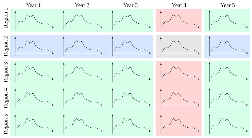
In the pool condition, we separated our influenza data series by seasons. To build forecasts for a region in a given season, the pattern library $\tilde{Y}$ included past and future seasons from all regions (including the one being forecast), while the data from any region and the same season was removed from $\tilde{Y}$. Note, first, that including such future examples of the season being evaluated is standard in EDM [14]. We expect that the causality between a year and the next one is fairly broken. Second, imagine that an important region would present some idiosyncratic dynamics during a season, which is later replicated in some other areas. This trend could serve as an indicator of what might happen in those adjacent regions with some delay. If we include all data from a given season, EDM could draw the inference in the opposite direction as well (using data of adjacent regions to forecast dynamics that had played out some weeks ahead). This is why, to be on the safe side, we removed all data from all regions for the season being forecast.

In condition classic, the library of patterns contained only examples from past and future seasons of a given region—which is how EDM was originally conceived [14] and how it has been applied, e.g., to forecasting flu trends in the past [15]. In condition annual, the library of patterns consisted of all the contemporary examples of a given region, ignoring all the examples from different years. This condition is proposed to measure the similarity between series from different regions in the same year, as the dominant flu strain will be the same and it might be possible for the effect of a region to be transmitted to a neighboring one within the same season. In Figure 2 we represent the three conditions.

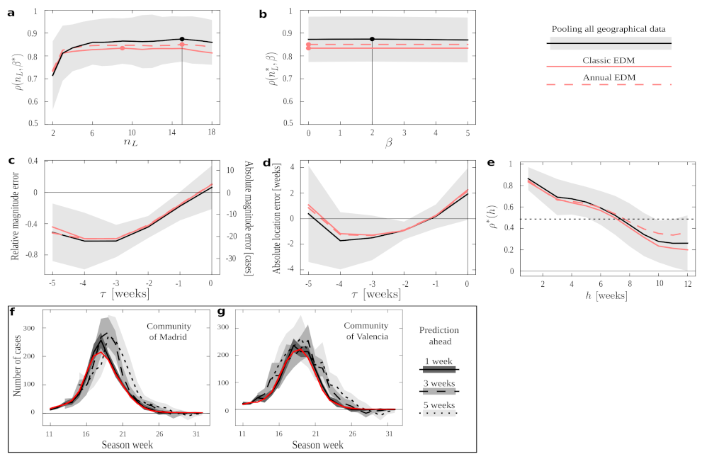
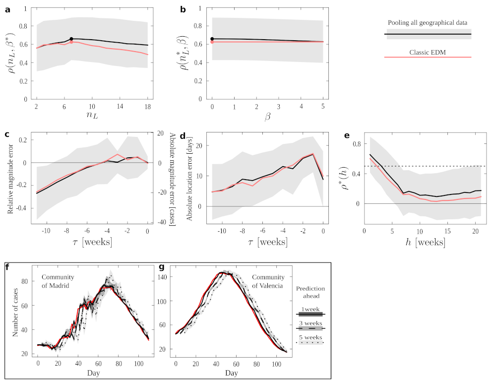
In Figure 3 we show EDM performance under the different conditions in a series of numerical experiments. If we keep $h=1$ fixed, we are simply trying to predict the next amount of new cases following the available data. We see the performance on this task with optimal ${\beta }^{*}$ and varying $n_L$ in Figure 3a; and for optimal $n_L^{*}$ and varying $\beta$ in Figure 3b. In both plots, condition pool outperforms all others in almost all the ranges explored and, most importantly, it does so for the optimal $n_L^{*}=15$ and ${\beta }^{*}=2$ (even for the optima derived independently for all other conditions, marked by filled red circles). Such optima would be the meta-parameters with which we should operate if we tried to forecast new time series not present in our data set—and in all cases the results suggest that we should use condition pool. Condition annual performs slightly better than the classic EDM, and both fall below pool. This demonstrates an overall advantage of pooling together epidemiological data across regions. This result might have been expected, since the pool protocol provides us with more data in our training set. However, it is not trivial that dynamics across regions (and, notably, having discarded series of a same season) would be informative to each other—each could have been affected by idiosyncratic factors such as population density, demographic structure, differences between urban and rural dynamics, etc.

The most important features that we would like to predict in an epidemic episode are how many people will be affected and how long it will last. The maximum height and location in time of the peak are a first proxy. To study how well we can forecast this, in a second experiment we aligned the data from all seasons taking each peak as a temporal reference. Then, we looked at how good the forecast of this peak was if EDM only had data until $\tau$ time units (weeks in the case of flu) before.

Figure 3c shows the average error (as relative and absolute magnitudes) that EDM makes in predicting the peak’s height. Figure 3d shows the error (in weeks) in predicting when the epidemics will reach its maximum. We appreciate that all protocols present quite similar curves. Thus, while pool produces better forecasts on average (as shown above), our results suggest that the uncertainty in predicting the magnitude and end of an epidemic process cannot be alleviated by more abundant data. This is in line with recent research [12] that shows how behind epidemic processes lie mathematical mechanisms that make them inherently unpredictable. Unfortunately, our non-parametric method cannot circumvent such problems.

Looking at these plots with greater detail, we see how errors become smaller as we get closer to the actual peak—as might be expected (however, observe the case for COVID-19). The smallest average error in magnitude happens as the data up to the very time of the peak is considered ($\tau =0$), while location is better predicted a week before the peak happens ($\tau =-1$). Error changes signs from negative to positive, meaning that EDM progresses (in average) from underestimating to overestimating. The forecast at $\tau =-5$ (which is the furthest from the peak that we can study with the available data) is more accurate than some others for peak magnitude and than many others for peak location. This effect is noteworthy for estimating peak location: this forecast degrades notably before becoming better—perhaps because the steepest phase of the exponential dynamics happens somewhere between $\tau =-5$ and $\tau =-1$. It is noteworthy, though, that this does not impact magnitude estimation as much.

With time series aligned with respect to their peaks as in the previous experiment, we also measured EDM performance (as captured by correlation between data and estimate) as a function of $\tau$. This way, we quantify how well our method works given that it is $\tau$ time units before or after the peak. Again, all protocols perform quite similarly in this experiment, with pool being notably worse than others in some cases. Figure 3e shows ${\rho }^{*}(h=1;\tau )$, which starts and ends close to 0 (i.e., forecast is of poor quality further away from the peak). Performance raises up to ${\rho }^{*}(h=1;\tau )\sim 0.5$ as the peak is approached, and remains at a similar level right after the peak before starting to decline gently. The dent at $\tau =0$ (performance becomes factually nil) is explained because the slope of the data series changes around the peak. Unless both data and prediction are perfectly synchronized (which, Figure 3d proves, is not the case), this leads to an average correlation of zero at that point.

Finally, it is relevant to establish for how long a forecast remains informative. Figure 3e shows the EDM performance, ${\rho }^{*}(h;n_L^{*},{\beta }^{*})$, as it tries to predict h time units ahead in time. Correlation remains above $0.5$ for predictions up to 7 weeks ahead of the available data, with pool being the preferred protocol in most cases. (Protocol annual becomes better around the time that correlation drops below $0.5$.) We show examples of how a relatively worse (Figure 3f) and better (Figure 3g) forecast degrade as we elaborate estimates with more time in advance. We see how this forecast degrades rapidly for a specific season of the Autonomous Community of Madrid, while it remains quite stable for some other seasons in the Community of València. This, together with the large deviations around most of the measures reported in Figure 3 (gray shadings), suggests that the right protocol might depend on the region studied, and that we might rather address this in a case by case basis. Below, we make some efforts to gain some insight about this issue.

3.2. Exploring EDM on COVID-19 Data

Data of the COVID-19 epidemic dynamics are affected by the various sources of unpredictability discussed above—some related to the unanticipated emergency caused by the pandemics, some others related to intrinsic properties of this malady and our social interplay with it. We have attempted to use EDM, pooling distributed geographic information from various sources, to forecast the dynamic unfolding of this crisis. Our success differed between more global (incorporating data from countries around the world) and local (as in our example from Spanish regions) attempts, and it changed over time as the pandemic changed as well. In this section, we report a brief example based on the same regions as above, now studying only conditions pool and classic. While far from successful, this attempt at forecasting allows us to quantify some aspects that reveal how the new virus unfolds with dynamics very different from those of seasonal influenza. Our data series in this case give us new infections per day, instead of weeks, so some results do not translate as readily.

Figure 4a shows the average EDM performance as a function of $n_L$ with fixed optimum ${\beta }^{*}=0$. We see an optimum $n_L^{*}=7$ (days), which is much smaller than the $n_L^{*}=15$ (weeks) found in the case of flu. This reveals how much more changing are the dynamics for COVID-19, and how informative patterns degrade more promptly as we attempt to compare them during longer stretches of time. This is indicative of a higher number of causal factors taking turns in dominating the dynamics—resulting in a more difficult forecast. Moreover, the correlation between estimates and prediction does not reach values comparable to those achieved with influenza data. Figure 4b shows EDM performance as a function of $\beta$ with fixed, optimal $n_L^{*}=7$. Again, we see how the pool condition renders better results.

We repeated the experiments to estimate the quality of peak forecast, but in this case taking into account that COVID-19 ‘waves’ are much more vaguely defined than seasonal peaks. Moreover, in some cases, EDM did not forecast the existence of a peak (suggesting, in turn, that the epidemics might grow unstopped within the time-window that we looked ahead). We report only results for cases in which a peak was predicted, and the comparison of its magnitude and location with that of an ongoing wave was possible.

Figure 4c shows that the error in magnitude becomes fairly small around 5 days before the epidemic peaks. By that time, EDM can produce an accurate first proxy of what the number of affected people will be. However, Figure 4d shows that the error in location of this peak only grows as we become closer to it. This is opposed to the results for flu, for which both magnitude and location estimates improved as the peak was approached. This indicates that EDM is consistently forecasting maxima that lie further away each time in the future of the approaching target and, in other words, suggests that COVID-19 waves do not show tell-tale signs that they are turning—thus aggravating the unpredictability of these kinds of dynamics.

The window of acceptable prediction capabilities is also much smaller for COVID-19 than for flu. Figure 4e shows how the correlation between estimate and data has already dropped below $0.5$ if we attempt to predict 5 days ahead. This is an insignificant forecasting window compared to the acceptable 7 weeks that we could look ahead with a similar accuracy in the case of flu. This points, once again, to the dynamical challenge posed by the SARS-CoV-2 pandemics.

Examples of forecast for the Community of Madrid (Figure 4f) and Community of València (Figure 4g) show very small deviations from their respective averages. This is due to the very scarce data available, which at the same time reveals a poverty of dynamical patterns to draw estimates from.

3.3. EDM as a Tool to Characterize the Epidemic Unfolding

Non-parametric forecasting methods are mainly results-oriented. They are often used as black-boxes—foregoing a deeper understanding of the dynamic process as long as forecasting works. This is the opposite, e.g., to compartmental modeling, in which causal relationships and meaningful parameters are inferred. With this later approach, insights can be gained about the relevant factors in the unfolding of an epidemic. However, we can turn EDM on its head, using its methods not as a predictor, but as a tool for correlating and clustering the dynamics across regions and years. Then: What regions are more informative to each-other? Can we reveal a spatial structure of how the flu or COVID-19 evolved in Spain? Are there idiosyncratic regions in which the dynamics play out rather differently? How do successive influenza seasons resemble each-other?

There is a question remaining, which is related to the fact that we are introducing data from several regions to predict another one: can we use EDM as a clustering tool?

To answer these questions we scored how often each region was within the nearest networks of each other region. Specifically, we count how many times a region takes examples from the time series of the rest of the regions to make the predictions, assuming that the dynamics of this region is related with the others. We also count how many times it takes examples from its own time series, which remarks that the dynamics of this region is different from the others. Thus, each element of the adjacency matrix $A_{ij}$ characterises the number of examples taken by region i from region j.

This helps us to generate a weighted and directed graph for all regions, which may be useful to study ongoing dynamics where there are not enough past data to make good predictions using other regions’ data. We applied this technique to both diseases—influenza and COVID-19.

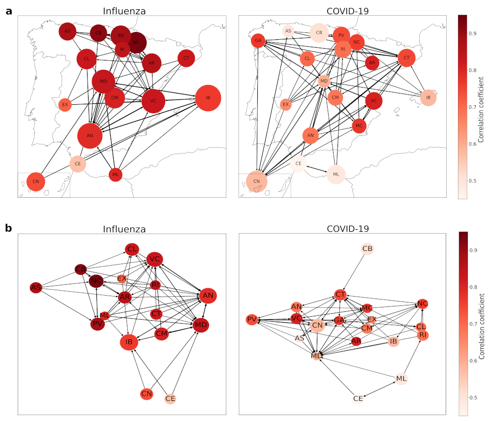
As it can be observed in Figure 5a, northern and central autonomous regions influenza dynamics are pretty well described with $\rho >0.85$, while the southern ones are one step behind not so far with $\rho$ around $0.8$ Andalusia (AN), Canary Islands (CN), Extremadura (EX), Melilla (ML) and Balearic Islands (IB) as well. Northern regions are also well connected between them and also with Andalusia, which even being at the south keeps a good relationship with other northern autonomous regions. This can be observed at Figure 5b, where we plot both influenza and COVID-19 networks with a random display, in order to visualize that well-described regions cluster together.

However, the main fact is that none of the considered regions takes more examples from themselves than from the other ones. If we have a look at the proportional number of neighbors chosen by the EDM for one region respective to the others, it goes from $2\%$ to $7\%$ of the total examples, with a mean of $4.0\%$ and a standard deviation of $1.6\%$ (the maximum $7\%$ is in the confidence interval of two standard deviations, so we can assume it is just a statistical fluctuation). This means these regions’ dynamics may be similar and EDM does not notice any region to be considered “special” from the others, as all of them take examples from other autonomous regions.

The final goal of this work was to develop a non-parametric prediction method capable of estimating new dynamics when there is no historical data available, such as in the case of the COVID-19 pandemic—as it is a new disease with very little information at its start. We tried to apply this method to COVID-19 data for several regions at a worldwide scale—country incidences—and at a Spanish autonomous regions’ scale, but the results were not as good as the ones obtained in influenza cases. This bad performance can be explained mainly in the lack of historical data, but also because the incidence over all territories have not been the same and not even comparable, as data cannot be scaled from one region to another and examples taken by EDM might not be true to reality. In addition, the quality of the data acquired from governments have not been the best, as at the pandemic start they were running out of tests and the infected people reports were not accurate enough [16].

This led us to compare how Spanish autonomous regions interacted with each other in this EDM approach considering COVID-19 dynamics from the first wave, from March 2020 to June 2020; the second wave, from June 2020 to December 2020; and part of the third wave, from December 2020 to February 2021, which ensures we have both ascending and descending trends, so EDM will be able to choose which one is better in each analysed case. For this reason, we repeated the clustering experiment for these data, and what we found out was there were many differences from the influenza epidemic network.

Having a look at the proportional number of neighbors chosen by the EDM—as we did in the section before—for one region respective to the others, goes from $1.7\%$ to $12.6\%$ of the total examples, with a mean of $5.1\%$ and a standard deviation of $3.3\%$.

There are some differences between the influenza and COVID-19 networks, but the most remarkable one is the fact that some regions take a large number of examples of themselves—in particular, Community of Madrid (MD), Valencian Community (VC), and Andalusia (AN). Correlation coefficients also reflect the bad performance of EDM predicting COVID-19 dynamics, as there are less well-described regions—-with $\rho$ over 0.85.

In terms of connections, we have a more dispersed network, where there is no clear clustering as we had in the influenza network. The northern regions are now more connected with the southern ones, so we could think of it as an insight of a different relationship of similarity than in the influenza case—which could be related to the geographical locations and similar weather, leading to comparable incidences due to the way of life people develop. Now we can observe that dynamics differ from the previous case studied, influenza, probably related to the differences in autonomous regions pandemic management, as they were mainly independent from the central government and they carried out different measures to stop the propagation of this disease, while influenza has been fought for many years and this leads to more homogeneous actions. Despite this dispersion, we can observe in Figure 5b the regions that are best described are centralized, as they are in the influenza network, denoting the potential application of this clustering method.

In summary, and taking all of this into account, there are several reasons why EDM is not able to perform well with COVID-19 pandemic data, but we can sum them up with two of them: lack of historical data and inhomogeneous disease incidences, which make the regions’ dynamics unpredictable from one to another.

4. Discussion

Among the many aspects that the COVID-19 pandemic has taught us, one clear lesson is the need to rethink modeling approaches to predict the spread of this kind of disease in the current world. This requires a diversity of approaches, including the creation of observatories analogous to the ones of meteorologists [17]. In order to do this, we need two ingredients: good data and good modeling tools.

Over the past century we have learned a lot about the dynamics that epidemics are very likely to follow. These happen to include exponential behaviors, such that the intrinsically correct models turn out to be extremely sensitive to the contingencies of real world data.

Real world data happens to have a lot of such contingencies (unknown causal factors that might be missed in the equations, errors in the collection of data, inconsistency of criteria in the recollection of data across time, etc). All of these trigger the sensitivity just discussed, in effect making it impossible to predict with the equations which, as we know, are very likely correct.

Non-parametric modeling offers a way forward. If a global observatory is established to track this and future pandemics, we should base it on the methods introduced by Sugihara and May [14] and further studied in this paper.

Our addition to these methods, including pooling data from different regions in order to enlarge the library of patterns to look at to make the forecasts, has proven to improve the results for both the cases of influenza and COVID-19—this idea has been also implemented successfully in other related works [18]. However, the problem of predicting the epidemic peak is still challenging for the new disease, as the new peaks tend to be quite different to the older ones, independently from the region, as COVID-19 strongly depends on different political measures to fight its spread, the initial conditions and dominant strains.

The uniqueness of COVID-19 dynamics can be observed in the difference its network presents in comparison with influenzas. While neighboring regions present similar performances for the latter, they show a lot more of heterogeneity in COVID-19’s network.

All analyses in this paper were based on the dynamics of the influenza and COVID-19 diseases independently. In expanding the observatory to potential epidemics in the future, we should contemplate the possibility of using the dynamics of a virus to attempt to predict the dynamics of another one (similarly to how here we use a region to predict another). This would provide very valuable information at the beginning of the pandemics. It might also help us understand what causal agents are behind an observed contagion process—e.g., does a virus present long incubation periods, etc.

Moreover, such an observatory should make use of other sources of information. For example, we know that SARS-CoV-2 RNA can be located in the feces quite early after infection. Such early warning would be extremely valuable in planning to cope with the epidemics.

5. Concluding Remarks

The complex behaviour of COVID-19 has raised the need of new modeling approaches to predict the spread of these kinds of diseases in our current world. Here, we have explored the possibilities of non-parametric modeling in the framework established by Sugihara and May [14]. The problem with this kind of approach when facing a new pandemics such as COVID-19 is the lack of previous sets of data to make the comparisons necessary to run the model. In addition to this, real world data are exposed to several contingencies (errors or different criteria applied in the recollection of data, unknown causal factors that might be missed in the equations, etc). Our proposal to solve these limitations is to add a pooling of data from different regions, with the idea of enlarging the library of patterns to look at to make the forecasts. We have conducted this with a known disease (influenza) and COVID-19, and the results point to a promising perspective. In this way, the establishment of a global observatory could offer a way forward for non-parametric modeling.

References

1. Iuliano, A.D.; Roguski, K.M.; Chang, H.H.; Muscatello, D.J.; Palekar, R.; Tempia, S.; Cohen, C.; Gran, J.M.; Schanzer, D.; Cowling, B.J.; et al. Estimates of global seasonal influenza-associated respiratory mortality: A modelling study. Lancet 2018, 391, 1285–1300. [Google Scholar] [CrossRef]
2. Cai, Y.; Li, J.; Kang, Y.; Wang, K.; Wang, W. The fluctuation impact of human mobility on the influenza transmission. J. Frankl. Inst. 2020, 357, 8899–8924. [Google Scholar] [CrossRef]
3. Stilianakis, N.; Perelson, A.; Hayden, F. Emergence of drug resistance during an influenza epidemic: Insights from a mathematical model. J. Infect. Dis. 1998, 177, 863–873. [Google Scholar] [CrossRef] [PubMed]
4. Casagrandi, R.; Bolzoni, L.; Levin, S.A.; Andreasen, V. Th sirc model and influenza a. Math. Biosci. 2006, 200, 152–169. [Google Scholar] [CrossRef] [PubMed]
5. Dool, C.V.; Bonten, M.J.M.; Hak, E.; Heijne, J.C.M.; Wallinga, J. The effects of influenza vaccination of health care workers in nursing homes: Insights from a mathematical model. PLoS Med. 2008, 5, e200. [Google Scholar] [CrossRef] [Green Version]
6. Dobrovolny, H.M.; Reddy, M.B.; Kamal, M.A.; Rayner, C.R.; Beauchemin, C.A.A. Assessing mathematical models of influenza infections using features of the immune response. PLoS ONE 2013, 8, e57088. [Google Scholar] [CrossRef] [PubMed]
7. Soo, R.; Chiew, C.J.; Ma, S.; Pung, R.; Lee, V. Decreased influenza incidence under COVID-19 control measures, Singapore. Emerg. Infect. Dis. 2020, 26, 1933–1935. [Google Scholar] [CrossRef] [PubMed]
8. Jones, N. How COVID-19 is changing the cold and flu season. Nature 2020, 588, 388–390. [Google Scholar] [CrossRef] [PubMed]
9. Lauer, S.A.; Grantz, K.H.; Bi, Q.; Jones, F.K.; Zheng, Q.; Meredith, H.R.; Azman, A.S.; Reich, N.G.; Lessler, J. The incubation period of coronavirus disease 2019 (COVID-19) from publicly reported confirmed cases: Estimation and application. Ann. Intern. Med. 2020, 172, 577–582. [Google Scholar] [CrossRef] [PubMed] [Green Version]
10. Byambasuren, O.; Byambasuren, O.; Cardona, M.; Bell, K.; Clark, J.; Mclaws, M.; Glasziou, P. Estimating the extent of asymptomatic covid-19 and its potential for community transmission: Systematic review and meta-analysis. Off. J. Assoc. Med. Microbiol. Infect. Dis. Can. 2020, 5, 223–234. [Google Scholar] [CrossRef]
11. Frieden, T.; Lee, C. Identifying and interrupting superspreading events-implications for control of severe acute respiratory syndrome coronavirus 2. Emerg. Infect. Dis. 2020, 26, 1059–1066. [Google Scholar] [CrossRef] [PubMed]
12. Castro, M.; Ares, S.; Cuesta, J.A.; Manrubia, S. The turning point and end of an expanding epidemic cannot be precisely forecast. Proc. Natl. Acad. Sci. USA 2020, 117, 26190–26196. [Google Scholar] [CrossRef] [PubMed]
13. Lorenz, E. Predictability: Does the flap of a butterfly’s wing in Brazil set off a tornado in Texas? In Proceedings of the American Association for the Advancement of Science, 139th Meeting, Cambridge, MA, USA, 29 December 1972. [Google Scholar]
14. Sugihara, G.; May, R.M. Nonlinear forecasting as a way of distinguishing chaos from measurement error in time series. Nature 1990, 344, 734. [Google Scholar] [CrossRef] [PubMed]
15. Viboud, C.; Boëlle, P.-Y.; Carrat, F.; Valleron, A.-J.; Flahault, A. Prediction of the Spread of Influenza Epidemics by the Method of Analogues. Am. J. Epidemiol. 2003, 158, 996–1006. [Google Scholar] [CrossRef] [PubMed] [Green Version]
16. Working Group for the Surveillance and Control of COVID-19 in Spain. The first wave of the COVID-19 pandemic in Spain: Characterisation of cases and risk factors for severe outcomes, as at 27 April 2020. Eurosurveillance 2020, 25. [Google Scholar] [CrossRef]
17. Press, W.H.; Levin, R.C. Modeling, post COVID-19. Science 2021, 370, 1015. [Google Scholar] [CrossRef] [PubMed]
18. Barreiro, N.L.; Ventura, C.I.; Govezensky, T.; Núñez, M.; Bolcatto, P.G.; Barrio, R.A. Strategies for COVID-19 vaccination under a shortage scenario: A geo-stochastic modelling approach. Sci. Rep. 2022, 12, 1603. [Google Scholar] [CrossRef] [PubMed]
Figure 1. Empirical time series of the influenza and SARS-CoV-2 epidemics. (a) Examples of historical time series of flu over 20 years in three Spanish regions: Basque Country (black), Community of Madrid (red), and Catalonia (blue). Data from each year (spanning from week 40 of a given year to week 20 of the next year) have been concatenated omitting the warm season (during which incidence is negligible). The gray area is expanded in (b) to show the yearly exponential raise, peak, and fall that characterizes the influenza cycle. Here, is data from 2015/16. (c) Evolution of the SARS-CoV-2 pandemics in the same three regions shows the pattern of waves within a single year, which are not always in phases across regions.
Mathematics 10 02494 g001
Figure 2. Illustration of different data pools for EDM. In grey, the example we want to forecast, is the testing series. In blue, is the method we call classic, which uses as library of patterns all the examples of the same region. In pink, is the method annual, which uses as library all the examples from the same year. In green, is the method pool, where we use the biggest library, taking all the series that are not from the same region or the same year.
Mathematics 10 02494 g002
Figure 3. Pooling geographically distributed information for influenza forecast. (ae) Results of different numerical experiments for conditions pool (solid black curves, with shading indicating standard deviation), classic (solid red) and annual (dashed red). Filled circles in (a,b) mark the location of optimal meta-parameters for each protocol. The optima for pool are also marked by vertical solid lines. Solid horizontal lines in (cf) mark the 0 of the vertical axis. Solid vertical lines in (ce) mark the location of the peak in time. Dotted horizontal line in f marks ρ * ( h ) = 0.5 . (a) EDM performance (as measured by correlation between data and forecast) as a function of n L with fixed, optimal β * . (b) EDM performance as a function of β with fixed, optimal n L . (c) Average error in forecasting the peak magnitude. (d) Average error in forecasting the peak location. (e) EDM performance as we attempt to predict more time ahead. (f,g) Examples of how the forecast become worst as we attempt to predict with more anticipation. Real data (solid red curves) is compared to forecasts derived with one week (solid black), three weeks (dashed black), or five weeks (dotted black) of anticipation. The various shadings indicate standard deviation of the estimated quantity. (f) Forecasts for the Community of Madrid. (g) Forecasts for the Community of València.
Mathematics 10 02494 g003
Figure 4. Pooling geographically distributed information for COVID-19 forecast. (ae) Results of different numerical experiments for conditions pool (solid black curves, with shading indicating standard deviation), classic (solid red) and annual (dashed red). Filled circles in (ab) mark the location of optimal meta-parameters for each protocol. The optima for pool are also marked by vertical solid lines. Solid horizontal lines in (cf) mark the 0 of the vertical axis. Solid vertical lines in (ce) mark the location of the peak in time. Dotted horizontal line in (f) marks ρ * ( h ) = 0.5 . (a) EDM performance (as measured by correlation between data and forecast) as a function of n L with fixed, optimal β * . (b) EDM performance as a function of β with fixed, optimal n L . (c) Average error in forecasting the peak magnitude. d Average error in forecasting the peak location. (e) EDM performance as we attempt to predict more time ahead. (f,g) Examples of how forecast become worst as we attempt to predict with more anticipation. Real data (solid red curves) is compared to forecasts derived with one week (solid black), three weeks (dashed black), or five weeks (dotted black) of anticipation. The various shadings indicate standard deviation of the estimated quantity. (f) Forecasts for the Community of Madrid. (g) Forecasts for the Community of València.
Mathematics 10 02494 g004
Figure 5. Influenza and COVID-19 networks. The size of the nodes is directly proportional to how many times a certain region has taken an example of itself. The darker a node is, the better it can be described—attending to the correlation coefficient ρ . Connection between generic regions A and B is plotted if the number of examples A takes from B overlaps 1.25 times the median number of examples A takes from other regions. (a) Geographical representation. (b) Graphical representation.
Mathematics 10 02494 g005
Publisher’s Note: MDPI stays neutral with regard to jurisdictional claims in published maps and institutional affiliations.