A Hybrid Artificial Intelligence Framework for Melanoma Diagnosis Using Histopathological Images

Abstract

Cancer remains one of the most significant global health challenges due to its high mortality rates and the limited understanding of its progression. Early diagnosis is critical to improving patient outcomes, especially in skin cancer, where timely detection can significantly enhance recovery rates. Histopathological analysis is a widely used diagnostic method, but it is a time-consuming process that heavily depends on the expertise of highly trained specialists. Recent advances in Artificial Intelligence have shown promising results in image classification, highlighting its potential as a supportive tool for medical diagnosis. In this study, we explore the application of hybrid Artificial Intelligence models for melanoma diagnosis using histopathological images. The dataset used consisted of 506 histopathological images, from which 313 curated images were selected after quality control and preprocessing. We propose a two-step framework that employs an Autoencoder for dimensionality reduction and feature extraction of the images, followed by a classification algorithm to distinguish between melanoma and nevus, trained on the extracted feature vectors from the bottleneck of the Autoencoder. We evaluated Support Vector Machines, Random Forest, Multilayer Perceptron, and K-Nearest Neighbours as classifiers. Among these, the combinations of Autoencoder with K-Nearest Neighbours achieved the best performance and inference time, reaching an average accuracy of approximately 97.95% on the test set and requiring 3.44 min per diagnosis. The baseline comparison results were consistent, demonstrating strong generalisation and outperforming the other models by 2 to 13 percentage points.

1. Introduction

Cancer is widely recognised as one of the most challenging diseases for physicians, due to its multifactorial complexity. Its genetic nature, rooted in DNA mutations and alterations, leads to high heterogeneity across cases. Additionally, environmental factors significantly influence tumour growth and progression, further complicating its diagnosis and treatment. Moreover, the variability in individual responses to cancer requires the adoption of personalised therapeutic approaches. Moreover, cancer requires a multidisciplinary approach, involving the collaboration of oncologists, surgeons, pathologists, and other specialists to provide comprehensive care. The diversity of cancer types adds another layer of complexity, with over 200 distinct forms identified [1], each demanding specialised expertise for proper diagnosis and treatment. Among these, skin cancer stands out as one of the most common forms in the United States, with its global prevalence continuing to rise [2]. Addressing this growing challenge requires significant efforts to advance diagnostic and therapeutic strategies tailored to the unique nature of skin cancer and its subtypes.

The most severe and potentially life-threatening form of skin cancer is melanoma [3]. Points out that in the United States, it is ranked as the fifth most common cancer in both men and women. It accounts for approximately 350,000 new cases and 57,000 deaths reported globally in 2020 [4]. The incidence increases with age, underscoring the importance of monitoring the population as it grows older. Survival rates for melanoma are closely linked to the stage of the disease at the time of diagnosis, making early detection a critical factor in improving patient outcomes and saving lives. While many melanomas are initially detected by patients themselves [5], clinician detection is often associated with thinner, more treatable tumours [6]. This highlights the value of professional screening in identifying melanomas at an early stage. For patients diagnosed with thin lesions and invasive melanomas (Breslow thickness ≤ 1 mm), treatment typically results in prolonged disease-free survival and, in most cases, a complete cure [7].

The current gold standard for melanoma diagnosis is histopathology, which analyses melanocytic neoplasms. These areas are tumours that originate from melanocytes, which are the cells responsible for producing the pigment in the skin. However, a subset of these neoplasms cannot be unequivocally classified as benign (nevus) or malignant (melanoma). These ambiguous cases are a significant source of diagnostic error, as evidenced by studies reporting discordance rates between expert dermatopathologists ranging from 14% to 38% using routine examination [8]. To reduce the risk of missing malignant lesions, the diagnostic criteria for melanoma have been adjusted to emphasise detecting as many potential cases as possible (sensitivity), even if this comes at the expense of a higher False Positive (FP) rate (reduced specificity). This trade-off highlights the urgent need for novel diagnostic tests that can increase accuracy by providing quantitative, objective information to minimise the inherent subjectivity of histopathological evaluation. Genetic analyses of melanocytic lesions have shown promise in distinguishing melanomas that harbour recurrent genetic aberrations absent in unequivocally benign lesions [9]. However, a “grey area” remains in histologically ambiguous melanocytic neoplasms with few genetic aberrations that continue to pose uncertainty regarding their biological behaviour.

Histopathologic diagnosis of melanocytic lesions is based on microscopic criteria including asymmetry, cytological atypia, deep maturation, pagetoid extension, mitosis and dusty pigmentation in melanocytes, which help the pathologist to classify these lesions as benign or malignant and to establish a specific diagnosis. Since these features may become ambiguous in some cases, expertise is most valuable in others. Doubtful cases are usually reviewed by several pathologists to arrive at the definitive diagnosis. This task is time-consuming and consumes significant resources due to the size and resolution of the images. Considering what has been mentioned previously, Artificial Intelligence (AI) techniques present a compelling solution to this problem.

By analysing big datasets, AI models can identify patterns in cases that are critical for human interpretation. These models can deliver diagnoses automatically and with remarkable speed, offering significant help in the accuracy and efficiency of melanoma diagnosis. AI is a discipline that aims to understand and replicate the mechanisms underlying intelligent behaviour in machines. This is achieved through various methods, which do not necessarily mimic the original biological mechanisms. AI encompasses a wide range of approaches, with Machine Learning (ML) being the most prominent in recent years. As defined by [10], ML is a field of study that enables computers to learn autonomously without explicit programming. It includes numerous techniques, where Deep Learning (DL) has emerged as a groundbreaking advancement. DL, as described by [11], refers to models capable of learning hierarchical representations of data through multiple levels of abstraction. These models are inspired by artificial neural networks, designed to emulate the behaviour of biological neurons. They achieve this through interconnected layers arranged sequentially, enabling them to process complex patterns and relationships within data effectively.

The primary motivation of this study is to develop a fast and accurate approach for diagnosing melanoma using histopathological images, aiming to speed up the diagnostic process for physicians. The proposed methods address the challenges associated with the high dimensionality of histopathological images, which require significant computational resources and complex feature extraction. To tackle these issues, we leverage the advantages of Autoencoders for enhanced feature extraction by reducing the dimensionality, combined with classical ML models for classification. Furthermore, the study incorporates a subjective evaluation to better understand the model’s performance and to identify common histopathological features that might confuse the classifier during diagnosis. This evaluation aims to bridge the gap between automated diagnostic tools and clinical practice, offering valuable insights to improve both the performance of the model and its interpretability for medical professionals.

The contribution of this work lies in the development of a workflow that first employs an Autoencoder for dimensionality reduction and feature extraction from histopathological images, followed by using these extracted features with various classifiers. This workflow produces a set of hybrid models that integrate novel DL techniques with classical ML algorithms. The performance of these hybrid combinations is evaluated both objectively, using standard mathematical metrics, and subjectively, through the insights of a medical expert in the field.

The innovation of the paper consists of the presented workflow and the different hybrid models, which, as far as we know, are the first time that these combinations are applied to diagnose melanoma using histopathological images. Moreover, the subjective evaluation lets us understand how the model works and what its limitations are.

The remaining sections of the paper are structured as follows. Section 2 provides a compilation of previous papers that pertain to the same field or share similarities with the proposed work. In Section 3, the data utilised for training the models and addressing the problems is described in detail. Section 4 presents the research findings and showcases the results obtained through the course of the study. Finally, Section 5 offers concluding remarks and highlights potential avenues for future research.

2. Related Works

As said above, in this work, different hybrid models using DL models alongside classical ML techniques have been proposed to diagnose melanoma with histopathologic images. Following, we compile different works using similar techniques for skin cancer diagnosis in general or melanoma.

First, we compile some works that only use classical ML techniques, for example [12] utilises Haar wavelet transformation in dermoscopy skin images to extract the main feature. These features are then introduced in different classifiers using the Random Forest (RF) algorithm, Support Vector Machines (SVM), or Naïve Bayes to discriminate between benign and malignant lesions. The same dataset is used in [13], where preprocessing techniques are used to eliminate noise and occlusion, such as body hairs. Then, some characteristics were obtained by applying the ABCD rule and using them to feed different ML models like SVM, RFs, and K-Nearest Neighbours (KNN). Another type of image to diagnose skin cancer is Optical Coherence Tomography (OCT), which is used by [14] to acquire both intensity and birefringence images of healthy and cancerous mouse skin samples. Using an SVM-based classifier, the researchers aimed to automatically distinguish images indicative of basal cell carcinoma (BCC), the most common type of skin cancer. Vibrational OCT is used with logistic regression and SVM to use telemedicine to classify between basal cell carcinoma (BCC), squamous cell carcinoma (SCC), melanoma, and controls [15]. In [16], different preprocessing techniques, including the Gray Level Co-Occurrence Matrix (GLCM), Principal Component Analysis (PCA), and fuzzy C-means clustering, extract features from skin cancer images, and then utilise SVM for diagnosis. Moreover, [17] integrates Matrix-Assisted Laser Desorption/Ionisation Mass Spectrometry Imaging (MALDI-MSI) with Logistic Regression (LR) to characterise and delineate cutaneous squamous cell carcinoma, achieving a predictive accuracy of 92.3% in cross-validation. Investigation by [18] focused on the role of triaptosis-related gene expression in melanoma prognosis by integrating single-cell and bulk RNA-seq data. A total of 101 ML algorithms and their combinations, including CoxBoost, Lasso, Random Survival Forest (RSF), and SurvivalSVM, were used to construct and validate prognostic models. The study presented by [19] combines 2D-IR spectroscopy and an ML algorithm called Partial Least Squares-Support Vector Machine (PLS-SVM) to classify melanoma patient serum samples, accurately predicting metastatic status and risk of relapse from protein fingerprint data. Finally, [20] applies Gaussian Naïve Bayes (GNB) and Logistic Regression (LR) to improve the histological classification of spitzoid tumours using Whole Slide Images (WSI) and clinicopathological features. To the best of our knowledge, the latter is the only work that utilises histopathological images in conjunction with classic machine-learning algorithms, although its primary aim is not melanoma diagnosis. In our case, we are not only using our dataset of histopathologies in melanoma, but we are also creating hybrid models that, apart from ML models, are using DL ones that face the problem of high dimensionality in this kind of image.

In the case of the DL models used to diagnose skin cancer, we have the following works where [21] uses different preprocessing techniques in images of skin lesions and evaluates how different CNN models (Resnet50, InceptionV3, and Inception Resnet) perform in diagnosing and classifying. Another work using CNN models is [22], where 11 different architectures were trained with a dataset that comprises 7 different skin lesions. After obtaining a model that performs well, it was also able to inform about the duration of sun exposure depending on the current UV radiation level, the individual’s skin phototypes, and the level of protection provided by the sunscreen used. Another CNN model is applied in [23], adding a shape-adaptive method to explain the diagnosis of melanoma through a heatmap. In the case of DL, papers are using histopathologic images. In [24], different pre-trained models like EfficientNetB0, MobileNetv2, ResNet50, and VGG16 were used to find squamous cell carcinoma (SCC). Moreover, [25] uses histopathologic images and DL models. VGG-16 with gradient-weighted class activation mapping (Grad-CAM), Otsu’s, and contour estimation, but in this case for the differentiation of skin melanocytes from keratinocytes. Another interesting work is [26], which evaluates DL melanoma classification using haematoxylin and eosin-stained WSI and immunohistochemistry-stained tissue slides using different ResNet models that were trained separately and jointly on these modalities. A study by [27] introduces a DL approach for melanoma prediction using Class-Agnostic Activation Maps (CAAMs), which enhance diagnostic reliability by addressing variability in lesion position and image transformations. The model was developed using ConvNeXt and ResNet backbones. Finally, [28] presents a multi-modal DL framework integrating dermoscopic images, histopathological slides, and genomic data for melanoma diagnosis using Convolutional Neural Networks (CNNs) for image analysis and Graph Neural Networks (GNNs) for genomic data interpretation. In these works, there are more similarities because we could find works using histopathologic images, but compared with our proposal, we proposed different hybrid models using DL and classical ML models for diagnosing melanoma.

As said above, one of the highlights of the present work is the hybridisation of models. In this way, we have found different works in the field of skin cancer [28] developed and validated a DL model to distinguish small choroidal melanomas from benign nevi using standard and ultra-widefield fundus photographs. The approach combined a two-stage U-Net architecture, one for lesion segmentation and another for melanoma risk scoring, with a shallow RF classifier trained on pixel-wise probability outputs [29] proposes a hybrid DL model that integrates ResNet50, Long Short-Term Memory (LSTM), and transfer learning to enhance skin cancer classification by capturing both spatial and sequential lesion features [30] combining a particular type of CNN called faster region-based with fuzzy k-means clustering to detect melanoma, and segmenting images of skin cancer lesions. A three-level method that uses DL in the first level, SVM, MLP, RF, and KNN in the second, and LR in the third level for classifying benign and malignant images of skin cancers is described in [31,32] presents a hybrid model called SCDNet, combining VGG16 with a regular CNN to classify between 4 different classes.

In the case of skin cancer that use hybrid models, we found [33] that combines multiple public datasets to enhance model training and optimising CNN parameters using the Artificial Bee Colony (ABC) algorithm to improve classification accuracy. Also, [34] presents a DL-based method for automated skin disease diagnosis. By hybridising CNN and DenseNet architectures, the proposed model achieves 95.7% accuracy.

Our approach differs from previous works by proposing four distinct hybrid models that combine DL and classical ML techniques for the classification of histopathological images as melanoma. In our workflow, the classifiers operate at the feature vector level, using latent representations extracted from the bottleneck layer of the Autoencoder. In addition to the standard objective evaluation using DL performance metrics, we also provide an expert-based assessment, offering a more comprehensive understanding of the model’s behaviour from a medical perspective. Furthermore, the two previously cited works reported lower accuracies of 93.04%, and 95.70% respectively, compared to our model, which achieves an accuracy of 97.95%.

3. Dataset Collection and Labelling

To train the proposed models, we collected a set of 506 histological raw images taken from 117 melanocytic lesions diagnosed between 2022 to 2023 at the 12 de Octubre University Hospital, including a wide spectrum of nevi and melanomas.

Whole-slide pictures were scanned at 200× with the Aperio Versa scanning system (Leica). Clinical data, including sex, age and location, were also collected. The age of the patient ranges from 10 to 89, with a percentage of 65.21% women, 30.43% men and 4.36% were not registered. Histological images were extracted from different parts of the body, including head and neck (33), trunk (35), Upper and lower extremities (40), metastases from deep tissues (6), and N/A (3 cases).

The labelling was performed by the three coauthors, histopathologists MGR, JLRP, and CPV, all of whom are expert dermatopathologists with extensive experience in the field. MGR and JLRP each have over 20 years of expertise, which is particularly valuable when diagnosing melanocytic lesions. All cases were independently reviewed by the three pathologists, using all available methods and clinical information.

The lesions included 31 melanomas (8 “in situ” melanomas, 12 superficial spreading melanomas, one acral lentiginous melanoma, 2 lentigo maligna melanomas, 7 melanoma metastases and one melanoma satellitosis) and 86 nevi (30 intradermal melanocytic nevi, 12 compound melanocytic nevi, 5 lentiginous nevi, 1 junctional nevus, 6 congenital nevi, 4 dysplastic nevi, 4 Spitz nevi, 9 Reed nevi, and 15 blue nevi). The hospital is officially categorised as a tertiary referral centre by the National Healthcare System. The present research has followed strict recommendations by the hospital Ethics Committee. In

Table 1. Summary of features of the collected dataset.

Dataset Feature	Values
Total raw images collected	499
Scanning magnification	200× (Aperio Versa scanner, Leica (Leica Microsystems, Wetzlar, Germany))
File format	Slide and Viewable Storage (.svs)
Bit depth/colour mode	24-bit RGB
Min., Max., Avg. image dimensions (pixels)	4583 × 6347, 91,683 × 170,804, 48,133 × 88,576
Min., Max., Avg. size dimensions (GB)	0.23, 9.41, 5.13

, we summarise the main features of the dataset.

4. Methods

4.1. Preprocessing the Histological Images

The raw images obtained from the scanned biopsies needed some transformations due to their large size and other circumstances arising during the collection. First, not all the obtained images were valid to train the models, as we found some problems, such as defocused images, others containing some physical labels that bring noise and other issues. At first, the raw dataset contains 499 images. At this moment, a curation process was carried out to ensure that all the images were accomplished with a minimum quality to be used by the models. In this way, a manual revision was carried out, dividing the dataset into five groups. Regarding the images from these groups, the following three were discarded due to insufficient quality. The first group contained 64 images that were out of focus. The second group comprised 47 images that were not fully scanned, with parts of the epithelial slice missing. Lastly, the third group had 67 instances containing text or physical labels that could introduce noise.

Of the remaining images, 321 in total were considered valid. However, we identified two distinct groups within this set. The first group contains 144 images with multiple epithelial slices scanned correctly. The second group consists of 121 images, where all the information is contained within a single slice. This set of 313 images was used to train the Autoencoder and the classifiers by randomly splitting them into an 80–20 ratio for training and testing. The training set for the classifiers includes 194 nevus images and 56 melanoma images. For the test set, this proportion consists of 49 nevus images and 14 melanoma images.

To augment the dataset due to the limited number of images, we generated synthetic data by rotating the original images, effectively increasing the dataset size by a factor of four. Consequently, the training set expanded to include 776 nevus images and 224 melanoma images. Similarly, the test set grew to include 196 nevus images and 56 melanoma images. This augmentation step was crucial in enhancing the model’s ability to generalise effectively.

After setting the training and test datasets, we realised that the images were too big, with sizes ranging from 6134 to 91,683 in width and from 5880 to 170,804 in height. This was a problem at the time of being processed by the models in terms of computational capacity and feature extraction (extracting more particular features is more difficult in big pictures). Due to this, the first decision was to crop the images into small pieces of the same size that were later fed to the model. In this case, it has been decided to divide the images into 256 × 256 pixel-coloured slices with no separation or union between them. For each image, a different number of crops has been obtained as the raw images have different sizes and because we have all the crops whose percentage of white pixels (normally pixels with no information) is greater than 60, which differs from image to image. In some cases, crops corresponding to the right and bottom border of the original image are discarded as crops of 256 × 256 cannot be created. At this stage, the number of cropped images is 612,397. After introducing them into the models, we normalised them by using the Whole Slide Images (WSI) normalisation algorithm, which is a particular way for managing histological images [35].

This algorithm starts by sampling a group of pixels from the tissue region of the histopathological image. Then, it converts the sampled pixels from the RGB (Red, Green and Blue) colour space to the Optical Density (OD) space. This conversion helps to separate the stain information from the image. After that, it utilises an ACD (Adaptive Colour Deconvolution) model to estimate the concentrations of different stains in the image. ACD models are commonly used for stain separation in digital pathology. In the following step, the algorithm calculates a stain-weight matrix based on the concentrations obtained from the ACD model. This matrix represents the importance or weight of each stain in the image. ACD matrix and stain-weight matrix are used to obtain some components, which are combined with the Stained Colour Augmentation (SCA) matrix that provides a reference for the desired colour appearance. The final output is a colour-normalised version of the input WSI, where the colours have been adjusted to avoid perception differences among images.

4.2. A Framework of Hybrid Models for Melanoma Diagnosis

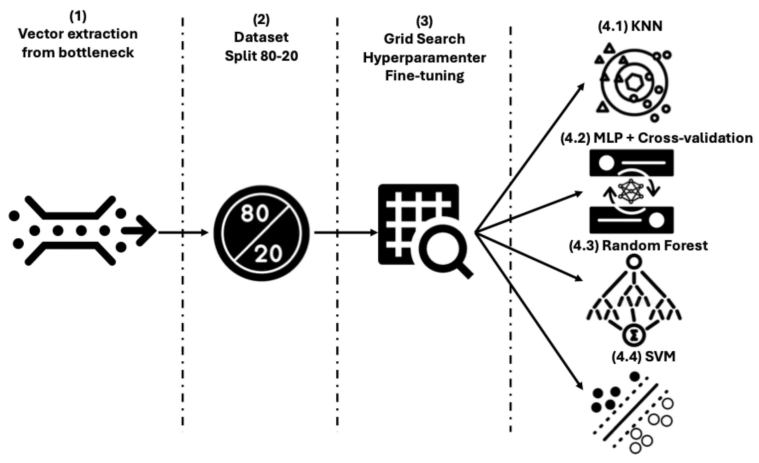
Once the initial dataset has been preprocessed, 4 workflows have been proposed to classify histological images into melanoma and nevus. They all follow the same 3-stage scheme, where the third stage changes depending on the final classifier that has been used. In the first part of the model, dimensionality reduction and feature extraction of the images are performed using an Autoencoder, which is trained to reconstruct each input image as output (this is the differentiated characteristic of the model among Encoder-Decoder models). Then, in the second step, these features are obtained from the bottleneck of the Autoencoder and are combined in 5 ways to introduce the features in the classifiers. This approach aggregates all the crops extracted from a single image during the preprocessing stage to generate a unified input instance for the classifiers, effectively representing the entire image. These combinations are made by obtaining the maximum values, the minimum values, summing them up, calculating the average values and the median. Finally, these vectorised features are introduced into different classifiers, creating the 4 models evaluated in this work. These classifiers are KNN, SVM, RF, and MLP. The workflow for the 4 approaches is shown in Figure 1.

The decision to use an Autoencoder over other solutions like pretrained CNNs is not obvious, but in the present use case, the latter approach has several limitations. In general, as pointed out by [29], self-supervised learning approaches such as Autoencoders can maintain satisfactory performance even when trained with as little as 1% of the available target dataset, making them particularly well-suited for domains like medical imaging where labelled data is often scarce. Talking about the use of pretrained CNNs, in [36] it is demonstrated that in smaller and less similar datasets like ours, applying transfer learning from unrelated domains often risks poor results. Following, we formally describe all the algorithms and methods used in the proposed workflow.

Autoencoders. This is a particular type of Encoder-Decoder model where the input and output instances during each epoch of the training stage are the same instance. These two-part models employ a process to capture complex structures. Initially, a multilayer encoder network is utilised to represent high-dimensional structures in a reduced-dimensional space. Subsequently, a decoder network is employed to convert the data from this space back into high-dimensional structures while maintaining certain relationships to the initial representation [37]. The functioning of this architecture can be described as follows: the input data traverses various convolutional layers within the encoder, extracting essential features and condensing them into smaller data fragments. These fragments are then organised within a bottleneck, forming a representation known as the latent space. Finally, the feature representation is passed through the decoder, resulting in an output that closely resembles the input data.

Autoencoders are formalised in [38]. During the encoding phase, an Autoencoder transforms an input vector X into a latent code vector Z through an encoding function f. In the decoding phase, the code vector Z is mapped back to a reconstructed output vector X′ using a decoding function g, to accurately reconstruct the original input. The Autoencoder adjusts the network’s weights W through fine-tuning, which is accomplished by minimising the reconstruction error L between the original input X and its reconstruction X′. This reconstruction error serves as the loss function used to optimise the network parameters. The objective function of the Autoencoder can be expressed as described in Equation (1).

$$\underset{\theta }{\mathrm{m}\mathrm{i}\mathrm{n}}{J}_{AE}\left(\theta \right)=\underset{\theta }{\mathrm{m}\mathrm{i}\mathrm{n}}{\sum }_{i=1}^n\left(x_i-x_i^{’}\right)=\underset{\theta }{\mathrm{m}\mathrm{i}\mathrm{n}}{\sum }_{i=1}^n\left(x_i-g_{\theta }\left(f_{\theta }\left(x_i\right)\right)\right)$$

(1)

where $x_i$ denotes the ith element of the input sample, $x_i^{’}$ represents the corresponding element in the reconstructed output, and n is the total number of training samples. The term l refers to the reconstruction error between the original input and its reconstruction.

Feature combination. Due to the large size of the images and the bottleneck, we have proposed different ways to combine the sets of these particular features so they can be introduced in classifiers. Once all the slices of the different images have been processed by the Autoencoder, the bottleneck will contain n slices (number of images, which is 96) of length m (number of features, 1,384,448, extracted by the Autoencoder). The length of these vectors is a consequence of the aggregation of latent features extracted from multiple 256 × 256 image crops. These vectors will be grouped depending on the image they belong to, and various operations will be performed to aggregate them. These operations could obtain the maximum, minimum, mean, sum, or median of each column of the vectors belonging to each image to create a single vector of length m per operation. Finally, we will have 5 vectors (one for each operation) of m characteristics for each image processed by the Autoencoder. These vectors will be the input data of the different classifiers. Feature aggregation operations are formalised in the following equations.

$$max\left(x\right){=max}_{x=1}^n{x}_i$$

(2)

$$min\left(x\right)={min}_{x=1}^n{x}_i$$

(3)

$$mean\left(x\right)={\displaystyle \frac{1}{n}}{\sum }_{x=1}^n{x}_i$$

(4)

$$sum\left(x\right)={\sum }_{x=1}^n{x}_i$$

(5)

$$median\left(x\right){=x}_{\left(k\right)where}{x}_{\left(k\right)}=⌈{\displaystyle \frac{n}{2}}⌉aftersorting\left\{x_i\right\}$$

(6)

In the equations above $x_i$ are part of a set of values ${\{x}_1,x_2,\dots ,x_n\}$ corresponding to a feature across $n$ observations or sub-elements.

K-Nearest Neighbours. Introduced by [39], presents an algorithm that assigns a class to an instance by considering the K-nearest instances from a given dataset. This approach allows KNN to assign a label based on the local patterns and similarities observed in the dataset. This label is assigned based on the KNN search, which is formalised in [38] as follows.

Let D be a dataset consisting of n points in a d-dimensional space, and let q be a query point in the same space. Let k denote the number of nearest neighbours to retrieve, and let dist (p, q) be a distance function that measures the distance between a data point p∈D and the query point q. The KNN search problem aims to identify a set R⊆D, containing k points, such that for every p∈R, there is no point p′∈D with dist (p′, q) < dist (p, q). In other words, R contains the k points in D that are closest to q.

Support Vector Machines. The current version of SVM was initially proposed by [40]. SVM can be conceptualised as a classifier that operates in an n-dimensional space, where instances are distributed. The primary goal of the algorithm is to locate a hyperplane that effectively separates individuals into distinct classes, maximising the margin of separation between them. The wider the margin, the better the classification performance of the SVM. By finding an optimal hyperplane, SVM enables the accurate and efficient classification of data points in higher-dimensional spaces. In [41], it is described as in Equation (7).

$$y\left(x\right){=w}^T\varphi \left(x\right)+b$$

(7)

In the equation above, $\varphi \left(x\right)$ represents the kernel function responsible for the feature transformation; essentially, kernel functions map the original feature space into a higher-dimensional space. In this transformed space, the features become linearly separable. The parameter b denotes the bias term, and the vector w is perpendicular (normal) to the hyperplane. The training input feature vector is denoted by x, while the classification of test feature vectors is represented by y(x).

Random Forest. As proposed by [42], ensemble learning is a method that leverages decision trees to improve predictive accuracy. This technique involves combining multiple decision trees and averaging their predictions, resulting in enhanced overall performance. One significant advantage of ensemble learning is its ability to mitigate overfitting, a common issue encountered when using individual decision trees. By aggregating the predictions of multiple models, ensemble learning reduces the likelihood of overfitting, leading to more robust and reliable results.

Formally, a RF is defined in [43] as a predictor composed of an ensemble of randomised base regression trees, denoted as $\{r_n\left(\mathrm{x},{\mathsf{\Theta }}_m,{\mathrm{D}}_n\right),m\ge 1\}$, where ${\mathsf{\Theta }}_1,{\mathsf{\Theta }}_2,\dots$ are independent and identically distributed (i.i.d.) realizations of a random variable $\mathsf{\Theta }$. These randomised trees are aggregated to produce the overall regression estimate represented in Equation (8).

$${\overline{r_n}(X,\mathcal{D}}_n)={\mathbb{E}}_{\mathsf{\Theta }}[r_n(X,\mathsf{\Theta },{\mathrm{D}}_n)]$$

(8)

where ${\mathbb{E}}_{\mathsf{\Theta }}$ denotes the expectation concerning the random parameter $\mathsf{\Theta }$, conditional on the input $X$ and the training dataset ${\mathrm{D}}_n$.

Multilayer perceptron. The Multilayer Perceptron (MLP) is a supervised neural network model that operates in a feedforward manner. It comprises an input layer and an output layer and can have any number of hidden layers that create a weight matrix. The fundamental MLP configuration typically includes a single hidden layer. Neurons within the network utilise nonlinear activation functions such as sigmoid, hyperbolic tangent, or Rectified Linear Unit (ReLU). The learning process is performed using backpropagation, employing the generalised delta rule to adjust the weight matrices. This iterative process updates the network’s weights, allowing it to learn and make predictions or classifications based on the provided input.

The computations performed by each neuron in the hidden and output layers are given by the following equations extracted from [44].

$$\mathrm{hr}=\mathsf{\Phi }\mathrm{r}=\mathsf{\rho }{v}_1\mathrm{g}\mathrm{r}+c_1$$

(9)

$$\mathrm{gr}=\phi (v_1\mathrm{h}\left(\mathrm{r}\right)+c_2)$$

(10)

where $v_1$ and $v_2$ are weight matrices, $c_1$ and $c_2$ are bias vectors, and $\mathsf{\rho }$ and φ denote the activation functions applied in the hidden and output layers, respectively. The set of parameters to be learned is given by θ = {$v_1$,$v_2$,$c_1$,$c_2$}.

4.3. Training Stage

The training stage is used to obtain the best performance of the models. First, data needs to be split into a train and test set in a proportion of 80/20. Then, we are applying two typical ML strategies: K-fold validation and grid search. We should highlight that, as non-neural models do not involve iterative training, they do not perform cross-validation

The different training approaches are evaluated with the two metrics, a loss metric for the Autoencoders and an accuracy metric for the. For the Autoencoder, our goal is to identify the model that best reconstructs the images. For the classifier, we aim to select the one that most effectively discriminates between the two classes in the dataset: melanoma and non-melanoma.

Cross-validation has been applied only during the training of the neural classifiers. K-fold validation is a technique used to evaluate statistical analysis results, ensuring their independence from the partitioning between training and test data. In our approach, the training dataset is divided into k subsets or folds. We perform k-training processes, with each process utilising a different fold as the validation set while the remaining k-1 folds are used for training. During each iteration, a different fold is selected for validation until all the folds have been used for this purpose. This process enables us to obtain multiple sets of results for the implemented metrics. To obtain more reliable estimates, we calculate the average values of the metrics over the k runs, along with the corresponding standard deviation. In our case, we divide the training set into 5 subsets, resulting in a 5-fold cross-validation. Each iteration involves training with 80% of the training set and validating with the remaining 20%. By following this methodology, we aim to achieve a reliable and unbiased evaluation of our model’s performance while mitigating the risks of overfitting and chance-based results.

Grid search techniques have been applied to optimise the Autoencoder and the classifiers. This is a technique that involves exploring a range of values for hyperparameters to identify the model with the highest accuracy [45]. This approach systematically combines various parameter combinations to thoroughly search the parameter space and determine the optimal configuration for achieving optimal performance. In

Table 2. Hyperparameters for the models.

Model	Hyperparameter	Values
Autoencoder	Learning rate	0.001, 0.0001
	Depth	6, 7, 8
	Number of kernels	4, 8, 16
KNN	Number of neighbours	3, 5, 6, 10, 12
	Weights	Uniforms, Distance
SVM	Kernel	Poly, RBF, Sigmoid
	C	0.01, 0.1, 1.0, 10.0
MLP	Hidden layers	4, 6
	Neurons in the 1st layer	128, 256
	Epochs	50, 70
	Dropout	0.3, 0.5
	L2 reg.	1 × 10−4, 1 × 10−3
	Batch size	32, 64
RF	Number estimators	80, 100, 120
	Split criterion	Gini, Entropy, Log Loss
	Maximum depth	33, 66, 100

, we compile the hyperparameters used to train the Autoencoder, KNN, SVM, MLP, and RF.

To summarise, the Autoencoders have been optimised via grid search, considering the best model to be the one that most faithfully reconstructs each input histopathological image, since the output is required to match the input. The grid search values in this step generate 64 different vectors (bottlenecks) that are combined according to the five functions of the feature combination algorithm. This operation generates 1189 input vectors fed into the six classifiers, which are fine-tuned according to different grid search strategies, generating 207 different test approaches. All of these combined generate 3105 accuracy values, which are evaluated by splitting the training and validation sets in an 80/20 ratio. In Figure 2, we schematically represent the previous process for the classifiers.

5. Results

The proposed solution combines two types of models. In the first step, Autoencoders are used for dimensionality reduction and feature extraction of the histopathological images. As this is a regression problem, we are using an error metric like the Mean Squared Error (MSE) as its capacity to measure the performance in feature extraction [46]. MSE calculates the average of the squared differences between the predicted values (reconstructed pixel) and the actual values (pixel in the original image). Equation (6) formalised this metric.

$$\mathrm{M}\mathrm{S}\mathrm{E}={\displaystyle \frac{1}{n}}{{\sum }_{k=0}^n\left(y_i-{\widehat{y}}_i\right)}^2$$

(11)

In this context, $n$ represents the number of data points (or examples) in the dataset. For each data point $i$, $y_i$ denotes the true (actual) value, while ${\widehat{y}}_i$ represents the predicted value generated by the model for that same data point.

Regarding this, MSE has been used to decide which set of hyperparameters performed the best in reconstructing the images. The following are the values of this metric in training, validation and test: 0.015233, 0.015333 and 0.01474. Complementary to the metrics, we attach Figure 3 with the diagram of lines for training and validation for MSE. This indicates good generalisation, which means that the model is not overfitting and performs similarly on unseen validation data as indicated by the previous values of the metric.

The chosen Autoencoder begins with an input layer that feeds the cropped 256 × 256 images into the first convolutional block of the encoder, which reduces the dimensionality of the images. The encoder consists of 7 convolutional blocks whose objective is to extract a feature map from the image. Each of these blocks has a 3 × 3 convolutional filter with a pooling layer of size 2 and stride 1. All filters apply the ReLU function as the activation function.

The number of filters in each block starts at 8 and doubles with each block, reaching 16 in the second, 32 in the third, and culminating in 512 in the seventh block. This gradual increase leads to a continuous reduction in the dimensions of the input feature map. As this reduction progresses, the input data, originally sized 256 × 256, is reduced to a size of 2 × 2. During this process, the essential features of the input image are meticulously represented in this compact information, effectively capturing the essence of the histopathology.

The next part of the model is the bottleneck, which comprises a convolutional layer with 512 filters. Throughout this part, the size of the feature map remains constant.

The model then progresses to the dimensionality boosting or deconvolution stage. This phase consists of seven deconvolution blocks, reflecting the number of convolution blocks. Each block consists of one upsampling layer followed by two convolution layers. Again, the number of filters within layers of the same block remains constant but varies between each block. Specifically, there are 512 filters in each layer of the first block, 256 in the second, 128 in the third, and so on until reaching eight filters in the final block. This progress serves to amplify the dimensionality of the feature map. During this deconvolution process, starting from the compact feature map at the bottleneck stage, the initial image used as input to the model is reconstructed, using only the features extracted from the original image. Figure 4 shows a representation of the Autoencoder.

As said above, many combinations have been performed to obtain the best results for each of the 4 classifiers. Following, we compile the best metrics in a table by using the accuracy, which measures the ratio of correctly classified instances to the total number of classified instances. It provides an initial indication of model performance and is often used as a starting point for evaluating the effectiveness of a model. To avoid the effects of randomness in the training and the separation between training and validation, we have obtained the mean and standard deviation of the 5-fold cross-validation. This information has been compiled in

Table 3. Accuracies for the four approaches.

Approach	Training Accuracy	Validation Accuracy	Test Accuracy
KNN + mean	100.00% ± 0.00	N/A	97.95%
SVM + mean	84.96% ± 0.00	N/A	75.00%
MLP + minimum	90.17% ± 6.00	85.69% ± 14.40	76.53%
RF + sum	100.00% ± 0.00	N/A	97.95%

. In the case of the test stage, the value corresponds to the fold that performs best, so it does not reflect the mean or standard deviation. Non-neural methods such as KNN, SVM and RF do not report a value at the validation stage. This is because no separate validation set was used during the training of these models. These algorithms do not rely on progressive, epoch-based training and thus do not require iterative monitoring of validation performance. Results in bold indicate the best performance.

Following, we give the values for the best combinations of vector aggregation operations with the hyperparameters for KNN and RF.

First, we explored different methods for combining the extracted feature vectors. In this case, the mean operation is the best for KNN and the sum operation for the best performing with RF. The best-performing KNN model uses distance weights, meaning that weights point to the inverse of their distance. Additionally, it uses a K value of 3, representing the number of nearest neighbours considered during classification. For the RF approach, it uses 80 estimators or created trees in the forest, the criterion to measure the quality of the splits is Gini, and the maximum depth of the tree is set to 33.

For an in-depth analysis of the models’ performance with FPs and False Negatives (FNs), we provide Figure 5. It contains the confusion matrices for the two best-performing models, KNN and RF, at the test stage.

Accuracy is a good way to measure the performance of a model. Otherwise, in cases of an unbalanced dataset and fields like medicine, it is essential to study how the model fails, reporting FPs and FNs compiled in confusion matrices and additional metrics such as specificity and sensitivity.

Specificity represents the ratio between the number of True Negatives (TNs) (non-melanoma states correctly identified as non-melanoma) and the total number of instances predicted as negatives (including both TNs and FPs, where melanoma is misclassified as healthy). Specificity is particularly useful in avoiding situations where patients are not notified of a potential melanoma, ensuring that timely intervention and treatment can be provided when necessary.

Sensitivity measures the proportion of actual positive cases (melanomas) correctly identified by the model. It reflects the model’s ability to minimise FNs, cases where melanoma is misclassified as nevi. This metric is particularly important in clinical settings to ensure that patients with melanoma are accurately diagnosed, allowing timely treatment and preventing missed diagnoses that could lead to severe consequences.

To further evaluate the balance between precision (accuracy of positive predictions) and sensitivity, we computed the F1-score, which is particularly relevant in the presence of imbalanced classes. It considers both the model’s ability to correctly identify positive cases (melanomas) and its precision in avoiding misclassifying healthy cases (nevi) as melanomas. A high F1-score is critical in medical diagnosis to ensure that most melanoma cases are detected over FPs.

Considering these metrics in melanoma diagnosis provides a more comprehensive assessment of the diagnostic performance, enabling a better understanding of the model’s ability to accurately identify melanoma cases while minimising FPs and FNs. The following Table shows these metrics for the best approach compiled in

Table 4. Specificity, sensitivity and F1-score for the best approaches.

Model	Training Specificity	Test Specificity	Training Sensitivity	Test Sensitivity	Training F1-Score	Test F1-Score
KNN	100.00% ± 0.00	95.55%	100.00% ± 0.00	100.00%	100.00% ± 0.00	97.93%
RF	100.00% ± 0.00	97.77%	100.00% ± 0.00	100.00%	100.00% ± 0.00	91.75%

.

In addition, we calculated 95% confidence intervals (CIs) for sensitivity and specificity to quantify the uncertainty associated with our diagnostic performance. This is crucial in the context of medical imaging and AI-assisted diagnosis, where robust performance must generalise beyond the test sample. For the KNN model, the sensitivity was 100% with CI (93–100%), and the specificity was 96% with CI (85–99%), demonstrating that it consistently detects melanoma cases with very few FPs. The narrow CIs indicate high precision and reliability of these estimates. By comparison, the RF model achieved a sensitivity of 96% with CI (87–100%) but a lower specificity of 65% with CI (52–76%), highlighting a greater risk of FPs.

Finally, to complement these metrics, Receiver Operating Characteristic (ROC) curves and Precision-Recall (PR) curves are useful as they provide a threshold-independent evaluation.

The ROC Curve is a graphical representation that illustrates the diagnostic ability of a binary classifier across various threshold settings. It plots the sensitivity against the FP rate. The curve provides insight into the trade-off between correctly identifying positive cases (melanoma) and incorrectly labelling negative cases (nevi) as positive. In medical contexts, the ROC Curve is valuable for evaluating a model’s performance independent of class distribution and decision threshold.

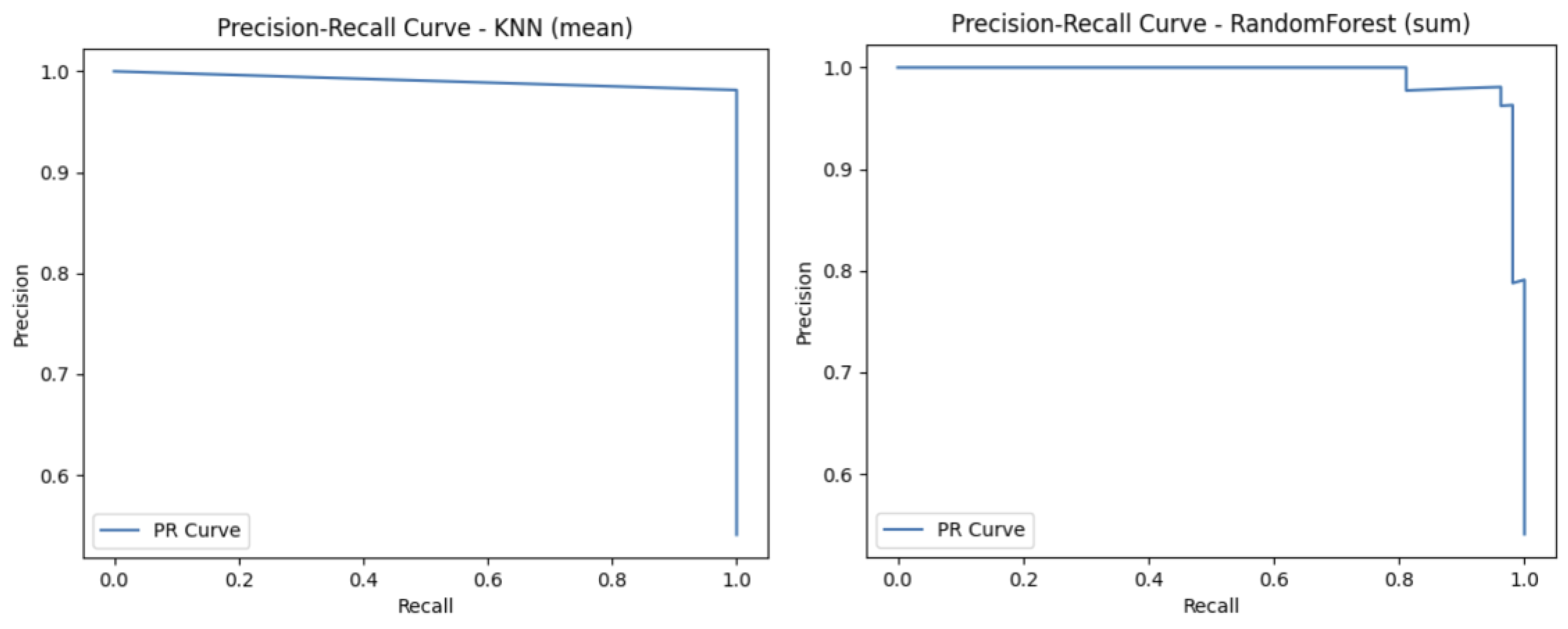
The Precision-Recall (PR) Curve is a performance evaluation tool particularly suited for binary classification tasks with imbalanced datasets. This curve plots precision against sensitivity, offering insight into the model’s ability to identify positive cases (melanoma) while minimising FPs (misdiagnosed melanomas). It is especially useful when FPs can lead to unnecessary treatments, and FNs carry severe health risks.

To complete the analysis with other metrics, we provide Figure 6 and Figure 7 that describe graphical metrics such as ROC-Curve and PR-Curve.

As mentioned above, one of the motivations for using hybrid models and extracting image features is the improved performance of Autoencoders for this task. To verify that we have compared our best approach to pretrained CNNs. This comparison has been made in terms of metric performance. We have compared our model to a well-known model used for image classification called ResNet50 [47]. Apart from that, three more baselines have been applied, which are the previous models using some of the hyperparameters obtained from the Autoencoder we have trained in this paper. This information is compiled in

Table 5. Comparison with baseline.

Model	Test Accuracy
Our model	97.95%
EfficientNetB3	85.71%
DenseNet121	95.24%
ResNet50V2	84.13%
EfficientNetB3 + Autoencoder hyperparameters	63.84%
DenseNet121 + Autoencoder hyperparameters	71.31%
ResNet50V2 + Autoencoder hyperparameters	62.24%

. Results in bold indicate that our method performs the best.

After demonstrating the good performance of our model, it is interesting to analyse its applicability in terms of diagnostic. In this way, regarding [48], the average time required to annotate WSIs that discriminate between melanoma and non-melanoma was approximately 15 min. By using our models, the average inference time per image was 3.44 min for the KNN classifier and 33.07 min for the RF model.

Finally, to quantitatively evaluate the quality of our model classification, we tested the performance of our classifier by comparing it to the diagnosis made by two histopathologists (as determined with all methods and information at hand) with the test set. The physicians who performed the evaluation are MGR, CPV and JLRP, who are expert dermatopathologists in the field and assigned the class labels. Diagnosis of melanocytic lesions is based on histopathological criteria, including asymmetry, cytological atypia, maturation, pagetoid extension, mitosis and dusty pigmentation in melanocytes, which the pathologist uses to classify these lesions as benign or malignant and to establish a specific diagnosis. Since these features may become ambiguous in some cases, expertise is most valuable in others. However, our strikingly accurate models (KNN and RF models) yielded 100% sensitivity and 95.55% specificity for the KNN classifier and 97.7% for the RF model, which means two cases were FPs with the KNN model and only one with the RF model. Coincidentally, both model fails to classify the same case (a deep blue nevus) as benign. The histopathological features of the two false-positive cases are compiled in

Table 6. Physicians’ evaluation.

Case	Asymmetry	Atypia	Maturation	Pegatoid Extension	Mitosis	Pigment
Pigmented lentiginous nevus (FP)	0	2	NA	0	0	3
Deep blue nevus (FP)	3	0	2	0	0	3

. The values range from 1 to 3, which means: 1 feature is fulfilled by nothing or very little, 2 features are fulfilled in some way, and 3 features are fulfilled by a lot or completely. In some cases, this value is NA (Not Available).

If we describe these two cases in detail, the first was a deep blue nevus showing a proliferation of spindled pigmented melanocytes in the deep reticular dermis. In the second case, there was a basal proliferation of pigmented melanocytes. These cases are difficult to classify even for physicians, as they share common characteristics with both nevi and melanoma. Therefore, it is understandable that the model could misclassify them. A potential solution to this problem is to increase the number of similar cases in the dataset, which could help improve the model’s ability to distinguish between these challenging examples.

To better illustrate how the model diagnoses, different pictures of the cases corresponding respectively to TNs, TPs and FPs are shown in Figure 8, Figure 9 and Figure 10. Figure 8 shows several examples of TN cases, including a case of dermal melanocytic nevus (Figure 8A), a Reed nevus (Figure 8B), a Spitz nevus (Figure 8C) and a dysplastic nevus (Figure 8D). Figure 9 shows two examples of True Positive (TP) cases, including a spreading superficial melanoma of 3.79mm of Breslow thickness with balloon degeneration (case A) and a superficial spreading melanoma, ulcerated of 5.5 mm of Breslow thickness (case B).

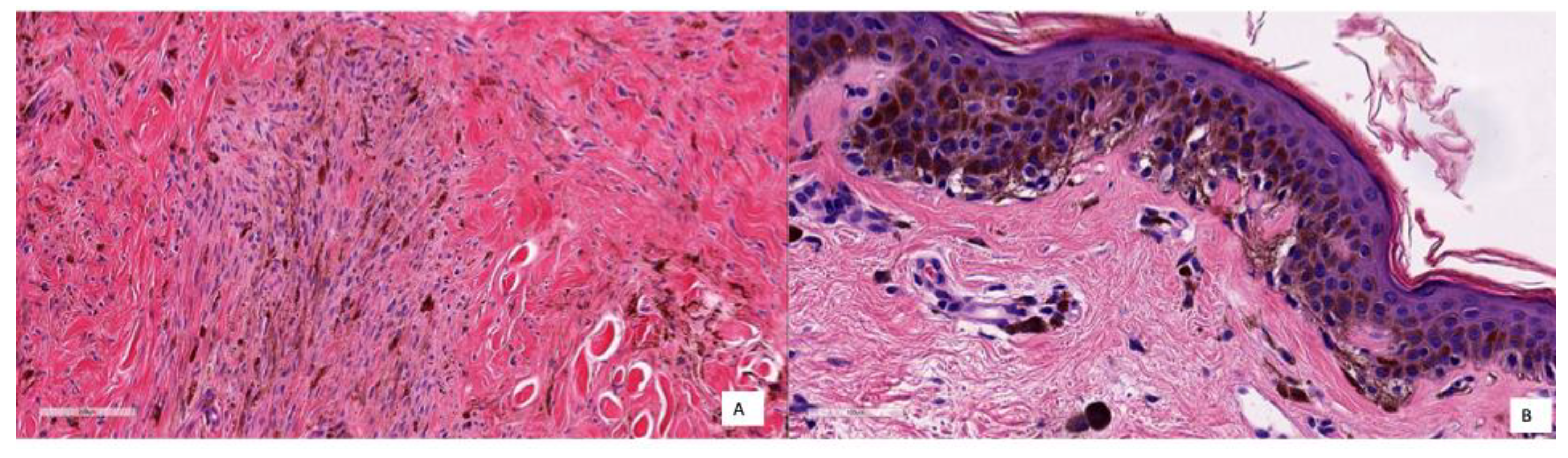
As said earlier, only two cases were classified as FP with the KNN model and only one with the RF model. Coincidentally, both models failed to classify the same case (a deep blue nevus) as benign. The histopathological features of the two FP cases are compiled in Table 5, and the images are shown in Figure 10. In Case A, the deep infiltration of the pigmented melanocytes and the spindled shape may be misinterpreted; in Case B, there is a basal proliferation of pigmented melanocytes.

6. Discussion

As can be seen in Table 3, the MLP and SVM classifiers exhibited comparatively lower accuracy. This can be attributed to the nature of the extracted features and the dataset limitations. Although the Autoencoder reduced the dimensionality of the histopathological images, the resulting feature vectors remain relatively high-dimensional, while the number of instances is small, a scenario that often leads to overfitting, as reported respectively for SVM and MLP in [49,50]. Analysing the rest of the results, the best classifiers correspond to the KNN and RF approaches, which are the ones we are considering as our final model to do diagnosis.

Regarding the performance of the model, if we look at the accuracy metric, the model accomplishes the bias-variance trade-off [51]. Some papers establish the accuracy of professionals diagnosing melanoma with histopathologies between 59 and 80%, depending on the experience [52,53,54]. In our case, this value is about 97.95%, which means an improvement of 17 points in the worst case. In terms of variance, the values could be considered good enough less than 3%.

Although accuracy is a good metric to obtain a first evaluation of how the model performs, an in-depth analysis can be obtained from confusion matrices and the other metrics: specificity, sensitivity and F1-Score. In this way, in Figure 5, we can see that the KNN model has two FPs and no FNs, and the RF has one FN and two FPs, demonstrating balanced sensitivity and specificity.

To complement the performance of the models, we obtained Table 4. In this case, the values in the test are very good for sensitivity, with no errors, which is good in the case of medical diagnosis, as no patient with cancer is considered healthy. Another interpretation can be obtained with the lower value that corresponds to the specificity. These problems with specificity could lead to a situation in which a healthy person could be diagnosed as having melanoma. Although this problem is not the most serious, it entails spending money on treatments that should not be applied and some consequences on the physical and mental health of the person receiving the treatment. The high F1-scores align with the perfect test sensitivity (100%) but are slightly lower than 100% because the test specificity is not perfect (95.55% for KNN and 97.77% for RF). In practice, a near-perfect F1-score like this suggests the model is highly effective at minimising both missed diagnoses (FNs) and unnecessary interventions (FPs), which is critical for patient safety, early treatment, and reducing undue anxiety in melanoma screening.

Regarding the CIs, they provide a range of plausible values for each metric, enhancing the reliability and generalisability of the results and supporting the conclusion that KNN offers a more balanced and trustworthy approach for melanoma detection in this context.

In summary, our model achieved exceptionally good performance in distinguishing melanomas and nevi with our set of cases, with a sensitivity of 100%, a specificity of 95–97% and an F1-Score from 91 to 97. These results outperform other ancillary tools with are frequently used by dermatopathologists for that purpose, such as fluorescence in situ hybridisation with a sensitivity and specificity of 87% and 96%, respectively [55] or comparative genomes hybridisation [9].

A final measure of the performance of the models can be carried out with Figure 6 and Figure 7, with the ROC and PR Curves. By analysing Figure 6, we can see that both models achieved an AUC curve of 0.99, indicating excellent discriminative performance. The KNN classifier exhibits a nearly perfect curve, suggesting minimal FPs and strong sensitivity. Similarly, the RF model maintains a very high TN rate and a low FP rate across thresholds. The proximity of both ROC curves to the top-left corner reflects a high ability to distinguish between classes (melanoma vs. nevi). An AUC of 0.99 implies that there is a 99% chance that the model will correctly rank a randomly chosen positive instance higher than a randomly chosen negative one. Overall, these results demonstrate that both models perform robustly and reliably in terms of classification capability. In Figure 7, both models demonstrate strong performance, maintaining high precision across nearly the entire range of sensitivity values. The KNN model exhibits a nearly flat PR curve, indicating that precision remains consistently close to 1 even as recall increases, suggesting that FPs are minimal across different thresholds. Similarly, the RF model also maintains high precision, with a slightly more variable curve toward higher recall levels, yet still preserving strong discriminative ability.

Compared with the baselines in the table, our model offers the opportunity for better quantitative modelling of disease appearance with a lower amount of input data and outperforms other CNN models such as ResNet, EfficientNet and DenseNet in the classification of melanoma and nevi. Even tuning these baselines with the optimal hyperparameters of the Autoencoder used in this paper, the results of our model are much better.

Considering all the results described above, we can conclude that the KNN model is the best choice, as it performs better in all metrics (accuracy, sensitivity, and F1-score) except for specificity, which is less problematic in this context. Additionally, the analysis of confusion matrices and confidence intervals supports its trustworthiness. Finally, the inference time further reinforces KNN as the most suitable solution.

However, some small limitations remain: the model is currently binary (nevus vs. melanoma) and does not support broader differential diagnoses; it operates on cropped image sections rather than full WSI, which may omit contextual information; and its performance has yet to be validated on external datasets or through prospective clinical studies. Apart from that, the key limitation of this study is the relatively small size of 14 melanoma cases in the test set, which affects the robustness of the sensitivity estimates. Such a small sample size may limit the generalisability of the findings. Therefore, caution is warranted when interpreting these results, and further validation on larger, independent, and more diverse cohorts of histopathological melanoma images is needed to confirm the diagnostic accuracy and clinical applicability of the proposed solution.

Another key consideration for the clinical translation of this type of diagnostic model is the need to address regulatory hurdles, system integration, and clinician training. From a regulatory perspective, AI-based diagnostic tools must undergo thorough validation and certification before being adopted in routine clinical workflows. Ensuring compliance with relevant medical device regulations and obtaining approval from health authorities is a necessary step before clinical deployment. Additionally, the integration of these tools into hospital information systems poses significant technical challenges, as compatibility with electronic health records and existing pathology software must be ensured. Seamless integration is crucial to allow clinicians to access AI-supported diagnostic results within their established workflows. Finally, effective clinician training is essential to maximise the benefits of AI systems. Healthcare professionals must be familiar with the capabilities and limitations of these models, and training programs should be designed to help them interpret AI outputs and incorporate them into their decision-making process. Without adequate training, there is a risk of over-reliance or misuse of AI-generated results. Addressing these regulatory, technical, and educational aspects will be critical for the successful adoption and clinical impact of the proposed diagnostic framework.

7. Conclusions and Future Works

The main aim of this work is the implementation of different hybrid approaches that use DL models and classical ML techniques for the diagnosis of melanoma using histopathological images. Apart from obtaining a model that performs this task accurately and improves the capacities of professionals in the field, we have provided a subjective evaluation that allows us to better understand model hits and misses in certain cases.

The workflow developed in this work comprises the following steps. First, images are cropped into smaller ones to avoid problems of computational capacity derived from the large size of the initial images. This stage also comprises the application of the WSI normalisation algorithm, a particular normalisation method developed particularly for managing histopathological images. After this, we applied a three-stage ML process for the diagnosis of the histopathologies. In the first stage, Autoencoders are used to obtain the most representative features of the images that allow for better discrimination between melanomas and healthy ones. Then, these feature vectors are aggregated by calculating the minimum of their values so they can be introduced into the ML algorithms. Even though different solutions were proposed, the two obtaining the best results were KNN and the RF algorithm. In this case, they obtain an accuracy of about 97.5%, which improves human performance by 9 points. This information has been complemented with other metrics, the calculation of CIs and the inference time. Regarding this, we can conclude that the best solution is the one using KNN

In future work, researchers aim to enhance the present diagnostic method. First, it is necessary to obtain a larger and more balanced dataset to mitigate the class imbalance issue. This will help determine whether current limitations are due to the dataset itself and may also offer insights for clinicians to improve disease diagnosis. Additionally, we propose implementing algorithms that replicate common tasks performed by dermatologists, such as counting mitoses and measuring the distance between the melanoma and the epithelial zone. Other complementary approaches—including the use of dual staining techniques or incorporating molecular analysis in complex cases—could also be explored to improve diagnostic accuracy. Lastly, to better understand how the proposed methods may fail in diagnosis, studies that provide a deeper analysis from a medical perspective are needed. In this way, the following research will include interobserver concordance comparing the performance of an AI classifying model with pathologists’ performance to highlight how digital pathology has the potential to augment the pathologist’s eye with objective information that cannot be gleaned by human examination.