Impending Doom: The Loss of Diversification before a Crisis

Abstract

We present four methods of assessing the diversification potential within a stock market, and two of these are based on principal component analysis. They were applied to the Australian stock exchange for the years 2000 to 2014 and all show a consistent picture. The potential for diversification declined almost monotonically in the three years prior to the 2008 financial crisis, leaving investors poorly diversified at the onset of the Global Financial Crisis. On one of the four measures, the diversification potential declined even further in the 2011 European debt crisis and the American credit downgrade.

1. Introduction

The purpose of diversification in a portfolio is widely understood from both a practical and a theoretical viewpoint. For example, Bodie et al. (2009, chp. 7), in common with many other authors, divide the total risk of an asset into two parts: the idiosyncratic risk and the systematic risk. Diversification is the grouping together of different assets in order to reduce the idiosyncratic or diversifiable risk, leaving a portfolio with, in the ideal case, only the systematic risk (see Bodie et al. (2009) Figure 7.1). However, Meucci (2009) points out “…there exists no broadly accepted, unique, satisfactory methodology to precisely quantify and manage diversification”.

In addition to being unable to precisely quantify diversification potential, there is the problem facing investors that the level of diversifiable risk, that is the risk that can be eliminated through diversification, does not appear to be constant but is time varying both within and between markets. A consequence of this problem is that, even if the assets held within a portfolio are not changed, the amount of diversification that a portfolio has rises and falls with changing market conditions.

Thus, there is need for tools to help investors understand how much potential for diversification exists to enable them to manage their portfolios effectively. A significant body of literature relavant to this topic already exists in two forms. One tries to directly assess the diversification potential that exists in a market or set of markets. For example, DeFusco et al. (1996) use co-integration methods to investigate the diversification potential in 13 emerging capital markets. The other is concerned with the estimation of systemic risk (not to be confused with systematic risk) (see, for example, Kritzman et al. (2011), Billio et al. (2012), and Zheng et al. (2012)). Much of the literature in this second group uses principal component analysis (PCA) for some of the work of estimation (see Jolliffe (1986) for a detailed description of PCA).

PCA is a standard method in statistics for extracting an ordered set of uncorrelated sources of variation within a multivariate system. Given that financial markets are typically characterised by a high degree of multicollinearity, implying that there are only a few independent sources of information in a market, PCA is an attractive method to apply.

Looking at the results of a PCA from a theoretical point of view, Kim and Jeong (2005) decomposed the correlation matrix of a selection of 135 stocks that traded on the New York Stock Exchange into three parts based on the Spectral Decomposition Theorem (for more information of Spectral Decomposition Theorem (see Jolliffe (1986, p. 13)). They assigned the following meaning to the principal components:

• The first principal component (PC1) with the largest eigenvalue represents a market wide effect that influences all stocks. In the financial literature, this is often called the systematic risk.
• A variable number of principal components (PCs) following the market component, which represent synchronized fluctuations associated with specific groups of stocks.
• The remaining PCs indicate randomness in the price fluctuations (noise). There were believed to contain no useful financial information and hence were eliminated from further investigation.

Systemic risk is defined as “the risk associated with the whole financial system, as opposed to any individual entity or component”. It can also be defined as “any set of circumstance that threatens the stability of financial system, and so potentially initiates financial crisis” (Zheng et al. 2012). For an investor seeking to manage a portfolio, rather than a regulator seeking to ensure financial system stablility, systemic risk can be thought of as the ratio of systematic risk to idiosyncratic risk. An increase in the systemic risk suggests that the systematic risk as a proportion of the total risk increases. Put another way, if the systemic risk increases, the amount of idiosyncratic risk, the diversifiable risk, as a proportion of total risk decreases, leaving the investor poorly prepared for any negative shocks to the financial markets.

After the financial crisis in 2008, literature relating to systemic risk has grown. There have been three groups of empirical studies on systemic risk.

• Literature focused on contagion, spillover effects and joint crashes in financial markets (Adrian 2007; Billio et al. 2012; Kritzman et al. 2011; Wang et al. 2011). Those studies were based on the analysis of interconnectedness among market security returns and our analysis below follows in their steps.
• Empirical studies on systemic risk that include research on the auto-correlation in the number of bank defaults, bank returns, and fund withdrawals (Brandt and Hartmann 2000; Kenett et al. 2012; Lehar 2005).
• Research on bank capital ratios and bank liabilities (Aguirre and Saidi 2004; Bahansali et al. 2008; Brana and Lahet 2009).

When the market becomes more connected, that is, the correlations between assets rises, the systemic risk is higher in the sense that shocks propagate more quickly and broadly. For this reason, monitoring the time evolution of the correlation between individuals stocks within a market and the correlation between markets is critical in portfolio management.

Other research has shown that the security correlations change in different time periods. Butler and Joaquin (2001) and Campbell et al. (2002) reported that the market correlation increased in bear markets. Ferreira and Gama (2004), Hong et al. (2007), and Cappiello et al. (2006) reached the same conclusions for global industry returns, individual stock returns and international bond returns.

Instead of comparing different time periods, many recent papers have applied PCA to investigate correlation using a sliding window approach. Fenn et al. (2011) applied PCA to study the evolution of correlation in a diverse range of asset classes. They asserted that increases in the variance explained by PC1 implied that there was more common variation in financial markets. Moreover, they emphasized that the variance explained by PC1 might be the result of either (1) increases in the correlations among a few assets or (2) increases in market-wide correlation. The first case will have less impact on the ability to diversify because an investor could simply move investments to less correlated assets. In contrast, it becomes much more difficult to reduce risk by diversifying across different assets if there is a market-wide correlation increase. For example, they reported that the sharp increase in variance explained by PC1 on 15 September 2008 was the case of a market-wide correlation increase precipitated by Lehman Brothers filing for bankruptcy and Merrill Lynch agreeing to be taken over by the Bank of America.

Kritzman et al. (2011) introduced a measure of systemic risk called the absorption ratio. It differs from the measure used by Fenn et al. (2011) in that it is the fraction of variance absorbed by a fixed, finite number of PCs rather than PC1 alone. They reported that most financial crises were coincident with increases in the magnitude of the absorption ratio. These crises include the Asian Financial Crisis in 1997, Russian default and LTCM collapse in 1998, the housing bubble in mid-2006, and the Lehman Brothers default in 2008. Another interesting finding in this paper is, in most cases, stock prices changed significantly when the absorption ratio reached its highest or lowest level.

Zheng et al. (2012) not only looked at the absolute value of variance explained by PC1, they also computed the change in the variance explained to capture the systemic risk. They reported similar findings to Kritzman et al. (2011) in that both the absolute value and change of variance explained by PC1 increased during a financial crisis. However, they reported that the moving window size and the time length used to calculate the change had an impact on the date of the spike. The spike of absolute value of variance explained by PC1 occurred later when the moving window size was larger and saturated after an approximately 20-month time window.

This paper adds to this literature by investigating two further measures of diversification (details in Section 2.2, Section 2.3, Section 2.4 and Section 2.5 below) and comparing them to existing measures. The Kaiser–Meyer–Olkin test of sampling adequacy is particularly simple to obtain at low computational cost and appears to be just as effective as a full PCA of the same data. Each measure could be generated on a daily basis to create a diversification potential time series index (or indices if more than one measure were used) in order to evaluate systematic changes over time. We confine ourselves to the Australian stock market but show, that within this market, the loss of diversification preceding the 2008 global financial crisis could easily have been detected well before the crisis hit. While the methods presented within this paper are only applied to a stock market, they are quite general and can used to assess the diversification potential across multiple asset classes.

The structure of the paper is as follows. Section 2 describes the data and methods, Section 3 contains the results, Section 4 contains the discussion and Section 5 the conclusions.

2. Data and Methods

This section is structured as follows; Section 2.1 describes the data we obtained and the preparation of the return series, Section 2.2, Section 2.3, Section 2.4 and Section 2.5 then describe the four methods of analysis that we applied to the return series. All four methods rely on analysing either a correlation or a covariance matrix, the generation of these matrices is described in Section 2.2. The first two methods, in Section 2.2 and Section 2.3, give us some insight into the connectedness of the market from which we can infer the diversification potential that is present. The second two, in Section 2.4 and Section 2.5, give us a more direct measure of diversification potential.

A rolling window approach was applied in our estimation process. We performed each analysis on a window size of two years (equivalent to 504 trading days) at weekly intervals. This resulted in 602 data points for each of our four analysis methods presented below.

2.1. Data

Our research is based on the Australian market. The main index for the market is the ASX200, which is a market capitalization weighted index of the 200 largest shares by capitalization listed on the Australian Securities Exchange. The index in its current form was created on 31 March 2000. We investigated the constituents of the ASX200 index from inception to February 2014. The ASX200 index is a capitalization index and so is not adjusted for dividends. In our research, we calculated the returns for all constituents that included the dividends paid.

There was a high frequency of stocks that were added to or deleted from the index from time to time, so we identified all stocks that had been in the ASX200 for the whole study period. After adjusting for mergers, acquisitions, and name changes, we obtained a final data set of 524 unique stocks. We obtained daily closing prices and dividends for each stock from the SIRCA database.1 All the prices and dividends were adjusted to be based on the Australian dollar (AUD). The return series was calculated from the price and dividend data (see Appendix A for details).

We extracted a set of stocks that had complete return information for the whole study period, and there were 156 such stocks. The remaining 368 stocks were either listed after April 2000 or delisted before February 2014.

2.2. Kaiser–Meyer–Olkin Test

Correlation and covariance matrices were generated from the return series with the cor and cov functions, respectively, in the stat package in base R (R Core Team 2014) on a rolling window of 504 trading days, which is equivalent to two calendar years. The correlation matrices were for use with the Kaiser–Meyer–Olkin (KMO) test described in this section and the two tests involving PCA. The covariance matrices were for use with the diversification ratio described in Section 2.5 below.

The Kaiser–Meyer–Olkin (KMO) measure of sampling adequacy (Kaiser 1970; Kaiser and Rice 1974) is calculated as

$$\mathrm{KMO}=\frac{\sum {\sum }_{j\ne k}{r}_{jk}^2}{\sum {\sum }_{j\ne k}{r}_{jk}^2+\sum {\sum }_{j\ne k}{q}_{jk}^2},$$

(1)

where the $r_{jk}$ are the original off-diagonal correlations and the $q_{jk}$ are the off-diagonal elements of the partial-correlation matrix. Thus, the KMO statistic is a measure of how small the partial correlations are relative to the original correlations, the smaller the $\sum {\sum }_{j\ne k}{q}_{jk}^2$ are, the closer the KMO statistic will be to one. A KMO value of $0.5$ is the smallest KMO value that is considered acceptable for a PCA.

We calculated the KMO statistic in rolling windows of different sizes for the 156 stocks that had complete data and settled on a window size of two years or 504 trading days as indicated above because this always gave a KMO value greater than 0.5.

The KMO test was performed using functions in the R package psych (Revelle 2014).

2.3. Principal Component Analysis

PCA can be applied to either a correlation matrix or a covariance matrix. All PCAs reported in this paper were carried out on correlation matrices.

PCAs were carried out using the function eigen in base R on a rolling window of 504 trading days. For a correlation matrix, the total variation is equal to the number of variables in the matrix. Thus, for our matrices, this was 156. To obtain the percentage of variance explained by PC1 if $E_1$ is the eigenvalue of PC1, then

$$\mathrm{Percent}\mathrm{Variance}\mathrm{Explained}=\frac{E_1}{156}\times 100.$$

(2)

2.4. PCA Stock Selection

Yang et al. (2016) presented a method for stock selection using principal component analysis. Their procedure is as follows:

• Apply PCA to the correlation matrix of a stock market.
• Associate one stock with the highest coefficient in absolute value with each of the last m principal components that have eigenvalues less than a certain numerical value, called the deletion criteria, and then delete those m stocks.
• A second or subsequent PCA is performed on the retained stocks. The same procedure described in step 2 is applied to the output of the PCA and, if necessary, further stocks are deleted.
• The procedure is repeated until no further deletions are considered necessary based on a stopping criteria that is a pre-determined minimum eigenvalue of the last principal component.

We used their procedure with a deletion criteria of 0.7 and a stop criteria of 0.5.

Intuitively, the procedure seeks to step-wise remove the most highly correlated stocks in the sample, leaving the most independent stocks. For example, if two stocks are highly correlated, they are likely to be found in the same high numbered PC each with a high loading. The procedure will then eliminate the one with the highest loading, leaving only one of the original pairs in the sample. From a diversification point of view, eliminating one of a highly correlated pair of stocks will result in only a small loss of diversification potential. Most of the potential will still be in the sample in the form of the retained stock.

2.5. Diversification Ratio

The diversification ratio is a measure of the degree of diversification for a long-only portfolio introduced by Choueifaty and Coignard (2008). The diversification ratio for a portfolio is defined as

$${\mathrm{DR}}_{\omega \in \mathrm{\Omega }}=\frac{{\omega }^{\prime }\sigma }{\sqrt[]{{\omega }^{\prime }\mathrm{\Sigma }\omega }},$$

(3)

where $\omega$ is the weight vector of the portfolio, $\mathrm{\Omega }$ is the set of investible assets, $\sigma$ is the vector of asset volatilities measured by their respective standard deviations and $\mathrm{\Sigma }$ is the variance–covariance matrix of the returns for the N assets. The numerator of the diversification ratio is then the weighted average volatility of the individual stocks and the denominator is the portfolio standard deviation. By this definition, the higher the diversification ratio, the better the degree of diversification. If a portfolio is completely non-diversified, in the case of single-asset portfolio, the diversification will achieve its lower bound of 1. The diversification ratio was calculated using custom written R code.

3. Results

The results are presented in Figure 1, Figure 2, Figure 3, Figure 4 and Figure 5 and discussed in turn in the sections below. They are presented in the order given in the previous section.

3.1. KMO Test

We discuss the KMO measure of sampling adequacy in Section 2.2. It is typically used prior to running a PCA to assess whether a PCA is worth performing (this was a serious issue when computing power was limited). Because in our sample it is a test of the degree of common variation among stocks, it gives us a tool to assess the market connectedness and therefore the potential for diversification.

Figure 1 presents KMO statistics from 2002 to 2014. For comparison purposes, the variance explained by PC1 is plotted on the same graph. A higher level of the KMO statistic indicates more common variation among stocks, which suggests less potential for diversification. We can see that the KMO statistic and the variance explained by PC1 evolved closely over time with a near-monotonic rise in both quantities in the three-year period (2005–2008) leading in to the Global Financial Crisis.

3.2. Market Wide Effects: Principal Component One

As indicated in Section 1, other authorities have used PCA to analyse market connectedness and systemic risk and have reported that financial markets have become more integrated during market crashes. We followed Fenn et al. (2011) and Zheng et al. (2012) and used the variance explained by the PC1.

Figure 1, Figure 2 and Figure 3 and Figure 5 each contain a plot of the variance explained by PC1. It is paired with the KMO statistic, the ASX200 index value, the index returns, and the diversification ratio, respectively. Figure 2 shows the index for the full study period. There are no results for the variance explained by PC1 in the first two years because that is the estimation period for the PCA. The value for variance explained has been plotted to coincide with the end of the estimation period. There was an almost five-year period from 2003 to 2008 in which the market steadily rose. The variance explained by PC1 began to steadily rise once the tail of the rolling window crossed the start of the rise. The rise was from a low of about five percent to about 20 percent close to the start of the financial crisis in 2008.

Figure 3 presents the same information as Figure 2 in a somewhat different form. The index values have been converted to estimation period returns. The index returns stayed high when the variance explained increased steadily from 2005 to 2008. Once the variance explained reach the first peak, the index returns started to drop significantly. The market remained tightly integrated until the beginning of 2010, even when index returns started to recover from the beginning of 2009. This suggests that the Australian stock market was still extremely fragile and therefore vulnerable to shocks during this period.

There was a small drop of variance explained at the end of 2010 while the index returns reached its second peak. The variance explained started to rise again at the end of 2011 and reached the highest point during the study period at the beginning of 2012. The reason for this increase of variance explained appears to be because of market-wide increases in correlation precipitated by the European sovereign debt crisis, and fears over the global economy. At the end of our sample period, the variance explained by principal component one had decreased significantly and the index returns had partially recovered from the drop in late 2011.

3.3. Number of Stocks Required for a Diversified Portfolio

The stock selection procedure described in Section 2.4 systematically selects a subset of stocks that are intended to maximise the diversification potential of the subset based on the correlations between them. However, the correlations between the stocks have changed over time and this affected the number of stocks selected. We hypothesised that during the periods of a more connected market there would be less risk sources. This means that, without altering the selection criteria, one should expect a smaller number of stocks being selected to describe the market. This is indeed what we saw.

Figure 4 presents the number of stocks selected. The results show a lot of fluctuation in the number of stocks selected. Nevertheless, consistent with the other results presented in this paper, the number of stocks selected decreased starting in 2006 and reached their lowest level in late 2009. The market had already become concentrated and offered fewer diversification opportunities before the 2008 financial crisis started. When the market became less tightly coupled, the number of stocks selected increased again.

This trajectory of number of selected stocks moved in an opposite way to the variance explained by PC1 (see Figure 2). This illustrates that the number of stocks needed to diversify a portfolio is not constant through time. With the number of major stock market risk sources changing, a portfolio can be considered diversified consistently only if it is adaptive to the change. In other words, the number of stocks included to diversify major risk sources should be changed based on the number of risk sources in the market. Thus, a portfolio that holds the same number of stocks or same constituents can only be the best combination to create a diversified portfolio at a single point of time. Holding more stocks than necessary when the number of major risk sources decreases is redundant. On the other hand, holding fewer stocks than required when the number of major risk sources increases means that the portfolio is under-diversified.

3.4. Diversification Ratio

The diversification ratio was discussed in Section 2.5 above. Recall that it is a measure of the degree of diversification for a long-only portfolio.

Because the purpose of this paper is to study how the potential for diversification has changed over time with the systemic risk, not to compare how different allocation strategies result in different degrees of diversification, we only present the portfolio with the most simple allocation strategy, 1/N. Figure 5 presents a plot of the diversification ratio for an equally weighted portfolio of all 156 stocks together with the variance explained by PC1.

The diversification ratio almost monotonically decreased with the increase in the variance explained by PC1. The diversification ratio dropped to its lowest point in our study period at approximately the same time the variance explained by PC1 reached its first peak. This suggests that even if an investor was holding the same portfolio, it would have become less diversified leading into the 2008 crisis.

Between the financial crisis in 2008 and the market decline in late 2011, the diversification ratio rose to about 3.75 at the same time the variance explained by PC1 dropped a little, but the diversification ratio was still 40% lower than it had had been between 2002 and 2005. If we look at Figure 3, we see that the index value recovered at the same time as the diversification ratio rose. Moreover, at the end of 2011, the diversification ratio dropped when the variance explained by PC1 rose. It is interesting that, even at the end of 2011, the variance explained by PC1 rose to its second peak and was higher than it was in 2008. The diversification ratio, on the other hand, while historically low, was not lower than in 2008.

4. Discussion

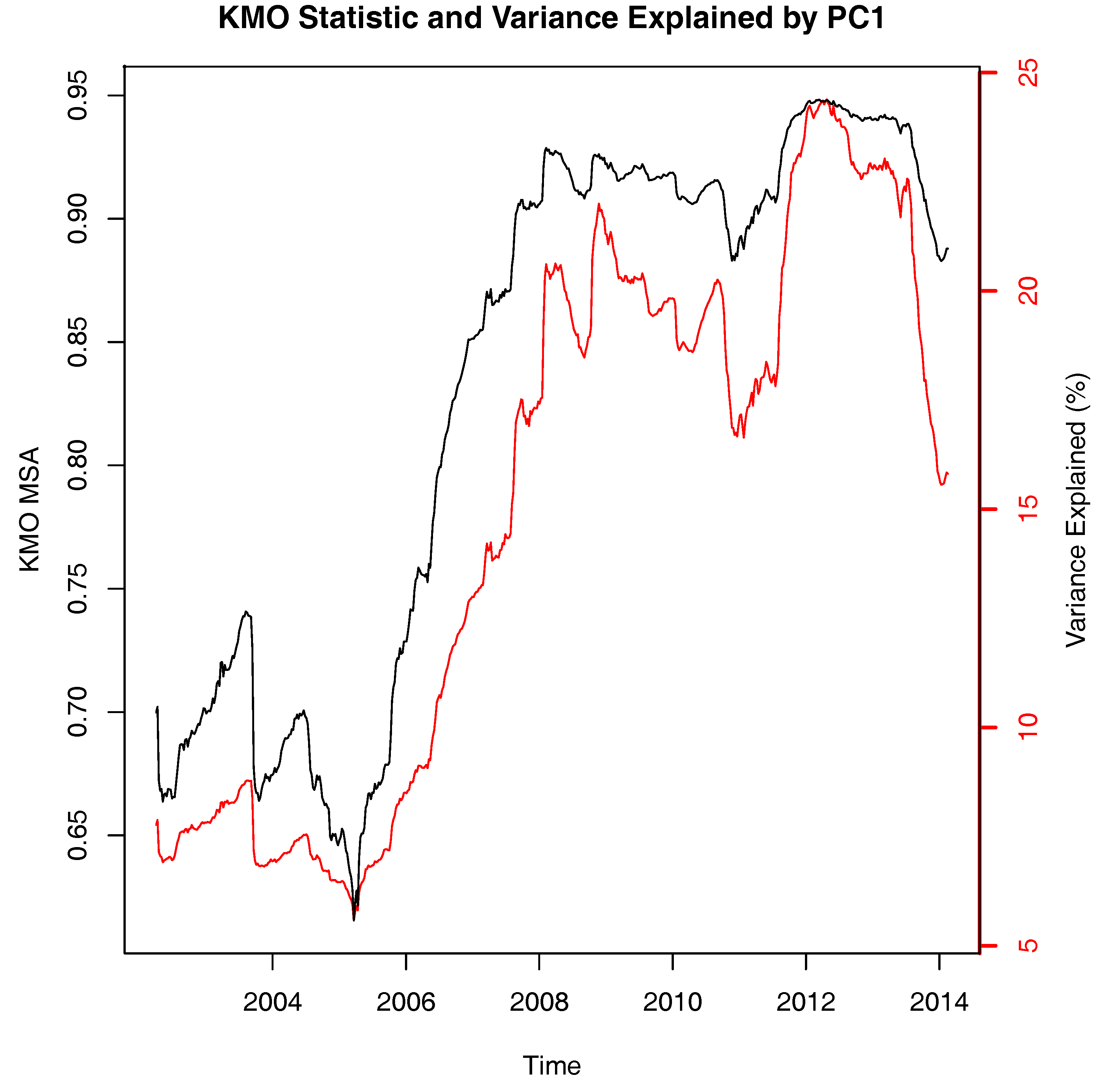
We have presented above four methods of assessing the potential for diversification in a single market. None of them answer the criticism of Meucci (2009) in that they do not directly quantify diversification potential. Nevertheless, as relative measures, their meaning is clear. Although they are not perfect substitutes for each other, they all show a consistent picture. This is perhaps unsurprising given that they are all based in some way on an analysis of correlation or covariance matrices. Of the four, the simplest to understand and easiest to use is the KMO test, which is typically applied to see if performing a PCA is likely to result in a significant reduction in the dimension of a data space. If we consider the return series for the 156 stocks in our sample to be a 156-dimensional data space, if the data is essentially a 156-dimensional hypersphere because each return series is uncorrelated with the others, then the KMO statistic will be zero or close to it, indicating a high potential for diversification. The further the data space deviates from sphericity, intuitively this means it becomes elongated in one or more directions because of common variation in returns, the higher the KMO statistic will be, hence indicating less potential for diversification.

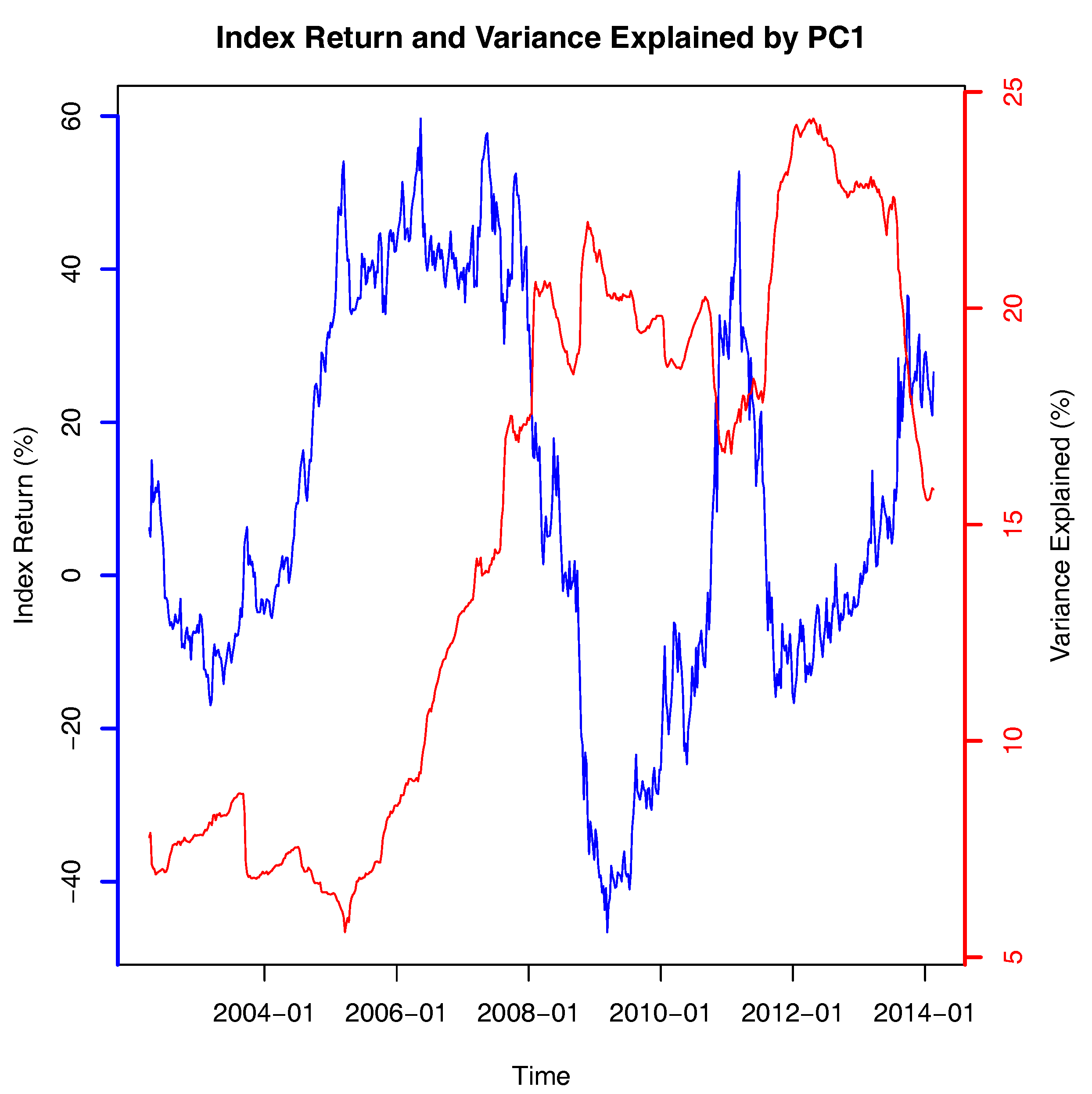
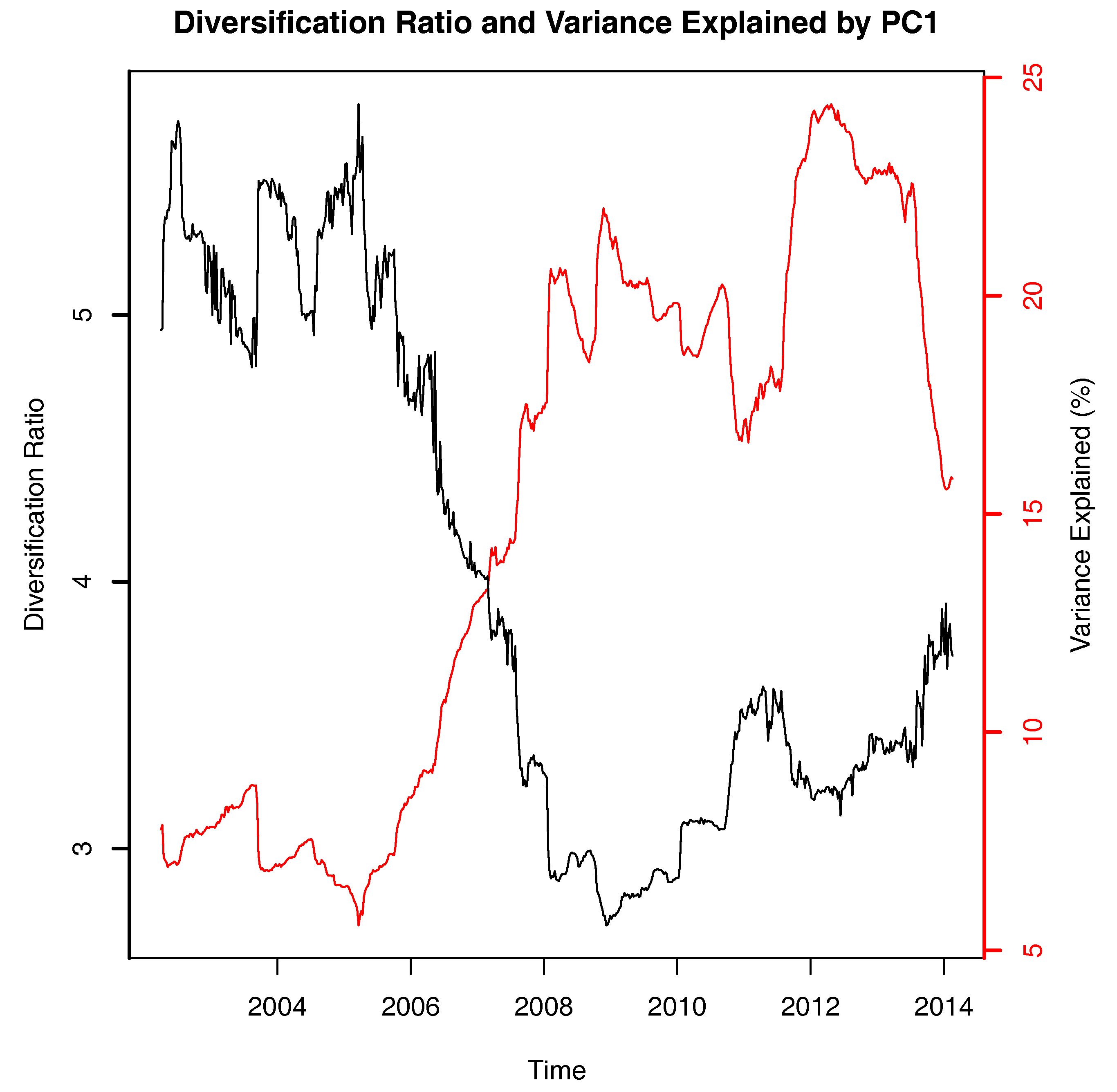
Sometimes this increase in common variation is referred to as an increase in market connectedness. From the results above, we can see the formation of a more connected market reduces the potential to diversify a portfolio. Many researchers have reported that markets offer less diversification in a falling than a rising market (Billio et al. 2012; Cappiello et al. 2006; Ferreira and Gama 2004). What our results show is that, when the Australian market was rising strongly, the potential for diversification was also decreasing. Thus, if an investor held a constant-sized small portfolio between 2003 and 2008, this portfolio became less diversified over that period and offered little protection when the crisis hit.

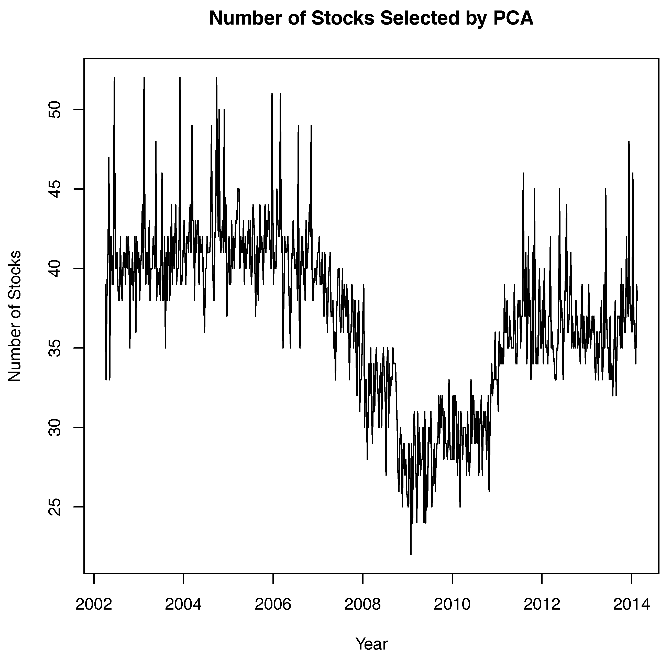
The results of the PCA stock selection procedure in Figure 4 initially appear counter-intuitive. Superficially it seems to be recommending that an investor hold fewer stocks when the market is more connected. It is, in fact, a more direct way to summarize the diversification potential in the market. In the period 2002 to 2006, it tells us that the 156 stocks in our sample, which we are using as a proxy for the market, could be summarized with approximately 40 well-chosen stocks. By 2009, those same stocks could be summarized in approximately 25 well-chosen stocks. Put in a more colloquial, but readily understandable manner, in the period 2002 to 2006, the market had approximately 40 stocks’ worth of diversification potential. By 2009, it only had 25 stocks’ worth of diversification potential. Thus, as the diversification potential declined, an investor who wished to hold a well-diversified portfolio would need to seek diversification opportunities in other asset classes to compensate for the loss of such opportunities in the Australian stock market.

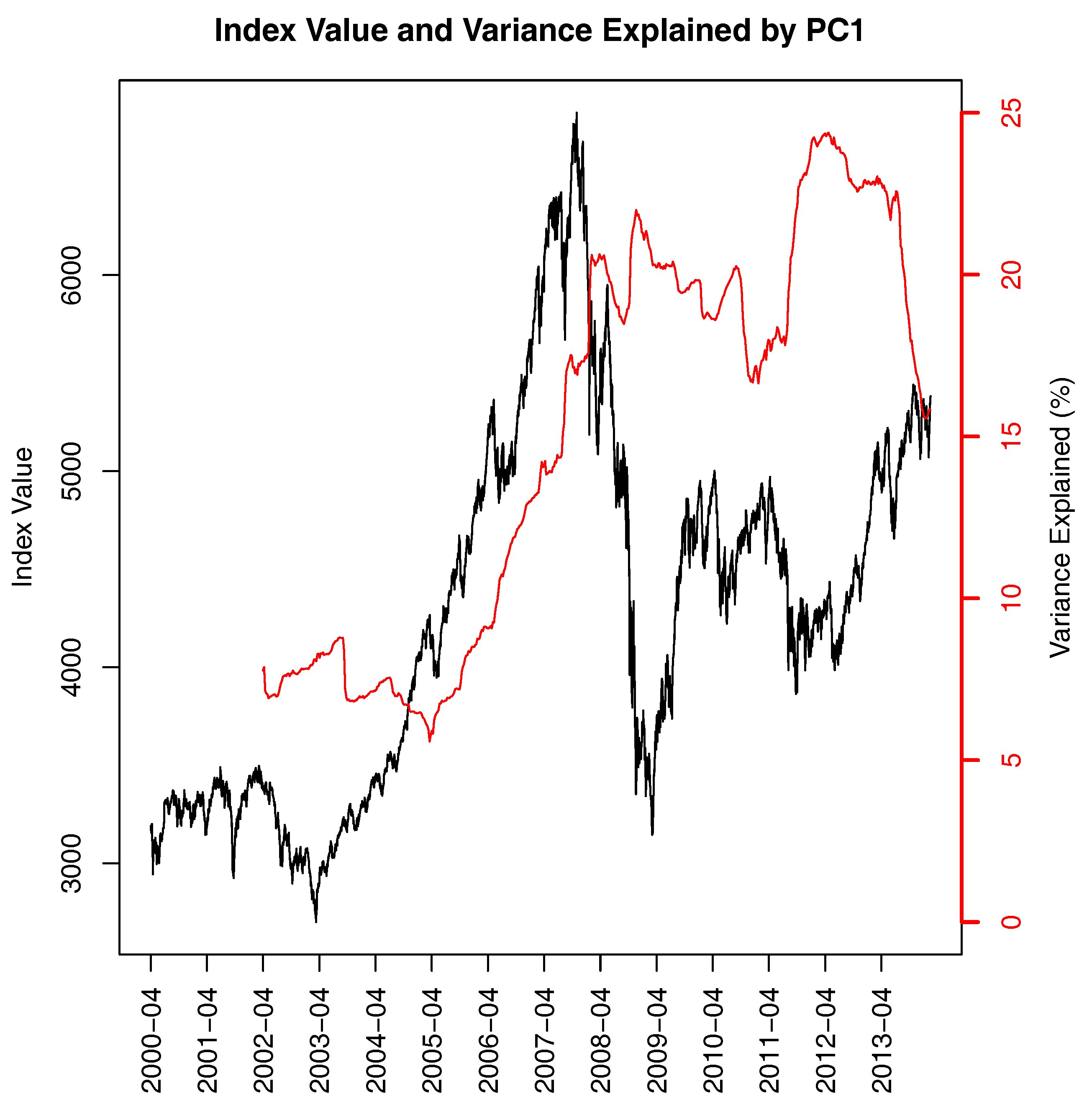
Portfolio management is conducted in a larger context than simply finding good stocks to buy. Our investigation suggests that, long before the global financial crisis happened, the market had become more closely connected and that this would have been fairly easy to detect. While all of the methods we have presented suffer from the need to have an estimation period, all of them would have indicated that the ability to diversify of a portfolio of stocks was declining well before it became a problem in the 2008 financial crisis. Both the diversification ratio and the PCA portfolio selection method showed that the potential to diversify within the market had decreased, that is, adding more stocks would not have added much diversification to the portfolio. The KMO statistic and the variance explained by PC1 rose indicating an increase in common variation within the market.

5. Conclusions

Our results in the Australian market supports the observations in many papers such as Kritzman et al. (2011), Zheng et al. (2012) and Fenn et al. (2011) that systemic risk increased steadily in the years before 2008. We also found an increase of systemic risk in the Australian stock market around the end of 2011, which coincided with the European sovereign debt crisis. These two observations are consistent with the study of systemic risk in the European market by Zheng et al. (2012). Our results are based on a similar testing framework to many other papers and adds two further supporting data points to the hypothesis that a large rise in the variance explained by PC1 may be a leading indicator of a financial crisis.

While the methods presented here were applied to a single stock market, they are, in fact, quite general and can be applied to any set of investment opportunities for which a correlation matrix (or covarinace matrix for the diversification ratio) can be generated.

As we have shown, it is straighforward to obtain and interpret each of the four measures of diversification potential discussed within this paper. While useful on their own, one or more of them needs to be incorporated into a wider portfolio selection and management framework. This should be a fruitful avenue of further research. To this end, the papers of Sawik (2008, 2012a, 2012b, 2013) provide methods of including additional selection criteria within the Markowitz Markowitz (1952) mean–variance portfolio optimization technique. It may be worthwhile trying to modify one or more of them to include measures of diversification potential as selection criteria in forming an optimal portfolio.