1. Introduction
Due to its low cost, lightweight, and high deployment ratio properties, the space membrane antenna can realize high-resolution observation of the earth with an extremely light load, which has become a promising antenna structure in radar remote sensing. However, the space membrane antenna also shows strong nonlinearity and flexibility, which makes its dynamic characteristics complex and vulnerable to external interference. The adjustment of its attitude and observation angle to the earth is one of the main factors causing the disturbance of its surface shape. Under the rigid–flexible coupling effect, the rigid body motion of the whole structure will have a great influence on the working performance of the space membrane antenna.
The nonlinear dynamics and response of membrane structures have been systematically studied in recent years. Zheng et al. [
1,
2,
3] investigated the free and forced nonlinear vibration responses of membranes under large displacement based on power series method, multiple scale perturbation method and Lindstedt Poincaré perturbation method. The results were compared with those under small displacement. Liu et al. [
4,
5] established the nonlinear dynamic models of large amplitude vibration of membranes by Krylov–Bogolubov–Mitropolsky (KBM) perturbation method and homology perturbation method (HPM), and proved the high efficiency of HPM by solving the model. Sunny et al. [
6] developed the dynamic equation of tensioned membranes under lateral dynamic load by using Adomian decomposition method. Fang et al. [
7] established a two-variable-parameter membrane model and solved the natural frequencies and mode shapes of the membrane antenna by distributed transfer function method (DTFM). Liu et al. [
8,
9,
10] conducted a series of studies on clamped membranes and tensioned space membrane antennas based on the modal assumption method and nonlinear finite element method. However, in the majority of the current researches, the membrane structures are assumed to have fixed boundaries, or the frames of the membrane antennas are fixed. In addition, the exciting forces on the membranes are always assumed to be local harmonic excitations or pulse excitations on the membrane surfaces. However, when the satellite/antenna adjusts attitude, the rigid motion of the satellite may cause the vibration of the membrane antenna because of its strong flexibility. Few studies have been done on these issues. Therefore, it is of great value to study the rigid–flexible coupling nonlinear dynamic characteristics of space membrane antennas under attitude adjustment disturbance.
At present, there are few researches on the rigid–flexible coupling dynamic characteristics of space membrane structures. In most studies, the space flexible accessories are simplified to flexible rod, beam and thin plate structures. Zhang and Deng et al. [
11,
12] established the rigid–flexible coupling finite element model of a spatial curved beam, taking into account the interaction between ‘rigid’ and ‘flexible’. Yoo et al. [
13] studied the influence of the motion-induced stiffness variation on the dynamic response of the plate, which is neglected in the conventional linear modeling method. Based on continuum mechanics, Fan et al. [
14] deduced the dynamic equations of a rotating flexible rectangular plate by using the Lagrange equation of the second type, and compared the first-order model with the zero-order model. Yuan et al. [
15] analyzed the coupling effect of translation and rotation of solar panels. Based on Hamilton’s principle, Liu et al. [
16] regarded solar panels as thin plates, established a discrete dynamic model through the global coordinate method, and compared it with the simulation results. Some other studies focus on the impact of the dynamic response of space membrane structures on satellites or other satellite accessories. Li et al. [
17] established the rigid–flexible coupling dynamic model of a solar sail. The dynamic responses of the hub tips under different maneuvering processes and different light pressures are calculated. Zhang et al. [
18] analyzed the influence of solar sail vibration on satellite orbit, attitude and its control torque through a rigid–flexible coupling model. Considering the Von-Karman nonlinear strain–displacement relationship of the solar sail, Liu et al. [
19] studied the influence of its rigid–flexible coupling effects on the pitching motion of the satellite.
There are also researches which put emphasis on model identification and the nonlinear behavior of nonlinear vibrations. Song et al. [
20] realized the model updating based on nonlinear normal modes extracted from vibration data via Bayesian interference. Luis et al. [
21] took an algebraic approach to identify the parameters of a class of nonlinear vibration, with Hilbert transformation criterion and calculus of Mikusinski applied. Habib et al. [
22] explored the relationships between nonlinear damping and isolated resonance curves. This work, by contrast, focuses on dynamic modelling of objects with a high degree of freedom, such as membrane antenna and investigates the rigid–flexible coupling effect during maneuvering of space appendages. The results can facilitate the intelligent control of large and complicated structures.
In this study, the rigid–flexible coupling nonlinear dynamic model of the space membrane antenna is established first using the finite element method. Then, based on the established model, the influences of rigid body motion and structural fundamental frequency on the dynamic response of the membrane antenna under a large range of rigid body motion are analyzed through several numerical examples. The results of this work lay a theoretical foundation for the in-orbit vibration suppression of membrane structures. Additionally, in contrast to the black-box-like operation of commercial finite element software, the proposed model can guide intelligent vibration control agent training, helping the finite element method play a role in the control of large and complex structures such as membrane antennas.
2. Nonlinear Dynamic Modeling of a Tensioned Membrane Antenna
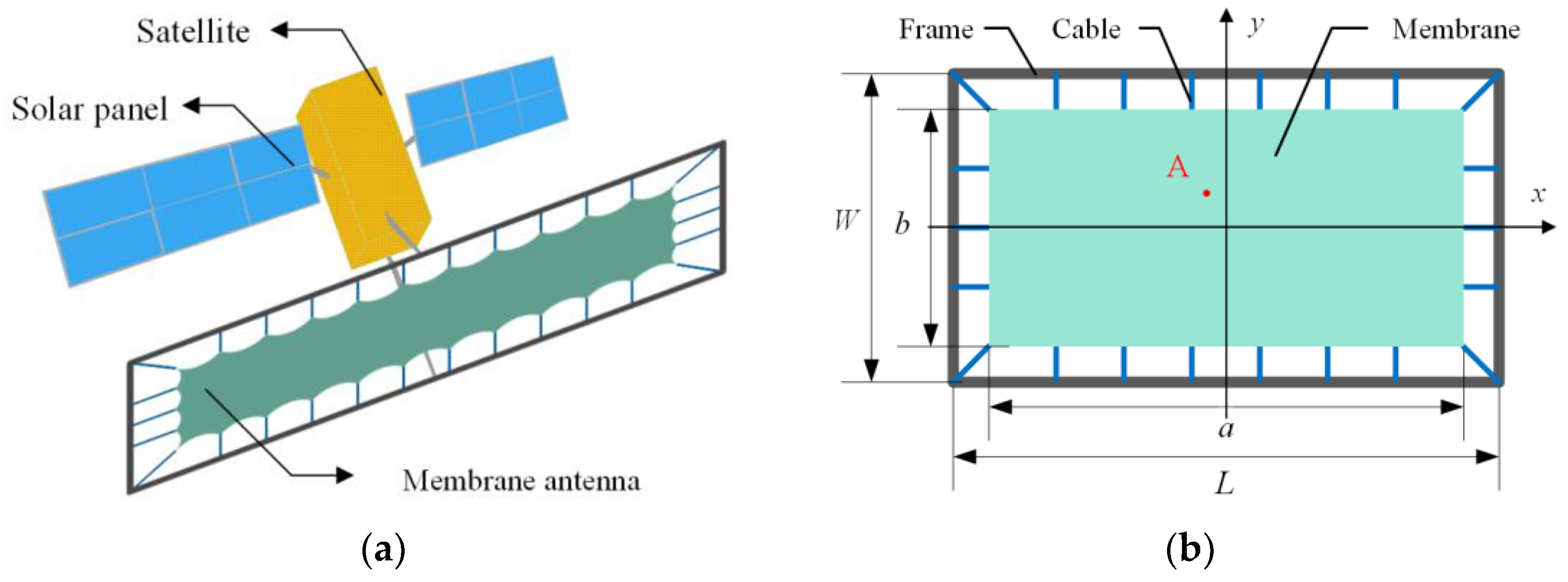
Figure 1 shows the schematic diagram of an in-orbit satellite with a deployable membrane antenna. Usually, the cutting lace of the membrane (see
Figure 1a) is to avoid wrinkles at the edge of the membrane, but this will introduce complex boundary conditions of the membrane. When the stress distribution on the membrane is relatively uniform, the lace will have little influence on the mode shape and frequency of the membrane structure [
23]. Therefore, in the modeling process, the lace-free tensioned membrane antenna, as shown in
Figure 1b, is adopted, which can simplify the boundary conditions. The membrane antenna consists of the thin-walled frame, the cables and the membrane. The whole structure is placed in the Cartesian coordinate system and the geometric parameters of each part are shown in
Figure 1b. In this section, the geometric nonlinearity and the rigid–flexible coupling effect of the space membrane antenna will be described, respectively.
2.1. Finite Element Model of the Membrane Antenna
In this paper, the finite element method is used to establish the dynamic model of the membrane antenna. The thin-walled frame, cable, and membrane are, respectively, equivalent to the Euler–Bernoulli beam element, pre-tensioned rod element and triangular membrane element. In this section, the displacement field of each element is shown in details.
For the thin-walled Euler–Bernoulli beam element, it is assumed that each node of the frame has six spatial degrees of freedom: a three-axis displacement
ub,
vb,
wb and a three-axis rotation
θbx,
θby,
θbz. Its displacement field
δb can be expressed by element shape function
Nb and element node displacement
qb as follows:
where
l is the axial length of frame element, and
e is the ratio of
x to
l.
For the pretensioned cable element, it is assumed that each node of the cable has three spatial degrees of freedom: three-axis displacement
uc,
vc,
wc. Its displacement field
δc can be expressed by element shape function
Nc and element node displacement
qc as follows:
where
e is the ratio of
x to the axial length of cable element.
For the triangle membrane element, it is assumed that each node of the frame has three spatial degrees of freedom
um,
vm,
wm. Its displacement field
δm can be expressed by element shape function
Nm and element node displacement
qm as follows:
where
Li,
Lj,
Lm are the area coordinates of a point in membrane element.
The following derivation and modelling are based on the finite element method, using the stated displacement fields.
2.2. Geometric Nonlinearity of the Membrane Antenna
In this paper, it is considered that flexible and thin-walled structures experience large displacement, but the relative deformation inside the element is still limited to small deformation, that is, the large displacement and small deformation problem. Taking second-order effect into consideration, geometric nonlinearity of the antenna will be described by geometric equations, physical equations and element potential energy. It has to be noted that gravitational potential energy is not included, as the membrane antenna is mostly applied in space.
2.2.1. Nonlinear Description of the Frame Element
Regarding the deformation of the frame element as a large displacement but finite rotation, the strain field of the frame beam element can be written as
where
where
and
are linear and nonlinear geometric matrixes of the frame beam element, respectively. It is considered that the material of the structure is linear elastic and isotropic. According to generalized Hooke’s law, the constitutive relation of the beam element is
where
σb is the element stress field,
Db is the elastic matrix of frame element,
Eb is the Young’s modulus of the material, and
Gb is the shear modulus of the material. Taking the variation of the element potential energy and then integrating it over time gives
where
Kbl and
Kbn are linear and nonlinear part of the stiffness matrix of the beam element, respectively, which can be expressed as
2.2.2. Nonlinear Description of the Cable Element
Since the cable extends only in the axial direction, only axial strain is considered in its strain field. In case of large displacement nonlinearity, the relationship between strain and displacement of cable element is similar to that of the frame beam element, which can be written as
where
sc denotes the nodal axial displacement,
is the strain of the element in
x direction,
is the axial strain, including the geometric nonlinearity caused by the lateral displacement. Then the axial strain of the cable element can be written as
where
where
Bcl and
Bcn are the linear geometric matrix of the cable element and the nonlinear geometric matrix caused by the second-order effect. Considering that the material of the structure is linear elastic and isotropic, according to generalized Hooke’s law, the constitutive relation of the cable element is
where
Ec is the Young’s modulus of the material. Since the cable is subject to pretension, the potential energy of the cable includes the strain energy caused by vibration and the initial elastic potential energy induced by pretension force. Taking the variation of the element potential energy and then integrating it over time gives
where
Kcl and
Kcn are linear part of the stiffness matrix of the cable element and the nonlinear part caused by the second order effect;
Kc0 denotes the equivalent stiffness matrix induced by pretension force;
QcΠ denotes the equivalent load vector induced by pretension force, which are expressed as
2.2.3. Nonlinear Description of the Membrane Element
Based on Kirchhoff’s thin plate hypothesis and Von Karman’s nonlinear theory, the relationship between the strain and displacement field of the membrane element can be expressed as:
where
where
εmx,
εmy and
γmxy are normal stress and shear stress of the membrane element in
x and
y directions.
Bml and
are the linear geometric matrix of the membrane element and the nonlinear geometric matrix generated by the interaction of in-plane and out-of-plane displacements. Since membrane structures belong to plane stress problems, the constitutive relation of the membrane element is
where
Dm is the elastic matrix of the membrane element,
Em and
μ are Young’s modulus and Poisson ratio of the material, respectively. Assume that the pretension stress of the membrane element is
Similar to the cable element, taking the variation of the element potential energy and then integrating it over time gives
where
Kml and
Kmn are the linear part of the stiffness matrix of the membrane element and the nonlinear part caused by the second-order effect;
Km0 is the equivalent stiffness matrix induced by pretension;
QmΠ is the equivalent load vector induced by pretension, which are expressed as
2.3. Rigid–Flexible Coupling Dynamic Model of the Membrane Antenna
The dynamic model of membrane antenna will be established in terms of Hamilton’s principle, which can be expressed as
where
T is kinetic energy;
Π is potential energy; and
W is the work done by external force on the system. In this section, the kinematic description will be given first, and the rigid–flexible coupling dynamic model will be therefore achieved.
When the space membrane antenna works in orbit, its attitude is mainly adjusted by the angle between the reflecting surface and the ground, i.e., the rigid body motion rotating around the
x axis (see
Figure 1) [
24]. Therefore, in this work, it is assumed that the membrane antenna rotates around the
x axis at a certain initial velocity and finally stops. Kane pointed out that for the rigid–flexible coupling effect caused by large-scale rigid body motion, the coupling term introduced by the influence of rigid body motion on the dynamic characteristics of elastic motion can be captured when considering the second-order nonlinearity [
25].
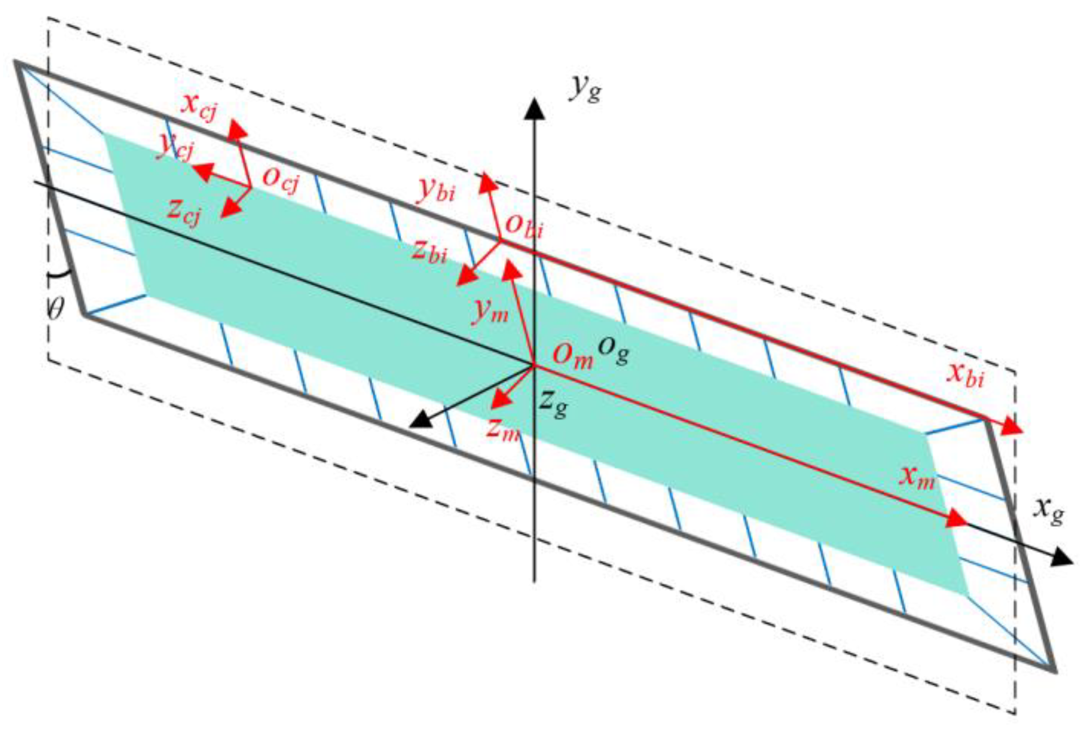
Based on this principle, a global coordinate system and a floating coordinate system are established on the space membrane antenna by using the mixed coordinate system method, as shown in
Figure 2, where
ogxgygzg is the global coordinate system,
obixbiybizbi is the floating coordinate system of the
i-th beam on the frame,
ocjxcjycjzcj is the floating coordinate system of the
j-th cable, and
omxmymzm is the floating coordinate system of the membrane. The rotation angle of the membrane antenna around
x axis is
θ, the rotation angular velocity and angular acceleration are
and
, respectively. The position vector of the origin of the floating coordinate system in the global coordinate system is
r0, and the spatial transformation matrix from floating coordinate system to global coordinate system is
A. Based on Hamilton’s principle, the rigid–flexible coupling nonlinear dynamic model of space membrane antenna will be established in this section.
The position vector
Rp of an arbitrary point
P on the membrane antenna in the global coordinate system can be expressed as
where
rp is the position vector of point
P in the floating coordinate system before elastic deformation;
Nq denotes the elastic deformation of point
P in the floating coordinate system. Furthermore, the velocity and acceleration vectors of point
P in the global coordinate system are written as
Taking the variation of the element kinetic energy and then integrating it over time yields
where
M is the element mass matrix;
G and
KT are the additional mass matrices caused by the rigid–flexible coupling effect, which exhibit damping and stiffness characteristics, respectively;
QT is the external load caused by the acceleration of rigid motion. When the rigid–flexible coupling effect is not considered,
G =
KT =
0, and Equation (41) degenerate to a general rigid body dynamic equation. The above matrices are specifically expressed as
For fixed-axis rotation, the spatial transformation matrix
A is the function of the rotation angle. Equations (43)~(45) can be turned into
where
α(
t) and
ω(
t) are the acceleration and velocity of rigid rotation, respectively.
G,
KT1,
KT2,
QT1,
QT2 are constant parts separated from
G,
KT,
QT. It is clear that rigid–flexible coupling effect is relevant with acceleration and velocity, which will be discussed in details later.
In
Section 2.1, the integration of potential energy of the frame, cable and membrane elements have been obtained, as shown in Equations (13), (21) and (32). The integration of kinetic energy of each element has also been obtained by using the mixed coordinate system method, as shown in Equation (40). Substituting the above equations into Equation (37), one can obtain the following rigid–flexible coupling dynamic equations of the frame beam element, the cable element, and the membrane element, respectively. By assembling the various matrices of all the elements, one can obtain the rigid–flexible coupling nonlinear dynamic equation of the space membrane antenna.
where the subscripts
b,
c and
m represent the frame beam element, cable element and membrane element, respectively, and the subscripts
0,
l,
n,
Π and
T represent the components related to pretension, linearity, nonlinearity, strain energy and rigid–flexible coupling effect, respectively.
M denotes the mass matrix,
C denotes the damping matrix,
F denotes the external load vector,
K denotes the stiffness matrix, and
Q denotes the equivalent load vector.
In this section, the influence of geometric nonlinearity and rigid–flexible coupling effect on the dynamic characteristics of membrane antennas is described theoretically. Instead of a merely numerical output, the expression of the theoretical model is more helpful to understand the nonlinear and rigid–flexible coupling dynamic behavior of space membrane antenna, so as to guide the dynamic design optimization and dynamic response control of the structure.
3. Solution of Rigid–Flexible Coupling Nonlinear Dynamic Response
In this paper, the Wilson-
θ method is used to solve the nonlinear dynamic equations. The model of the space membrane antenna is shown in
Figure 1, and the materials and geometric parameters of the membrane antenna are shown in
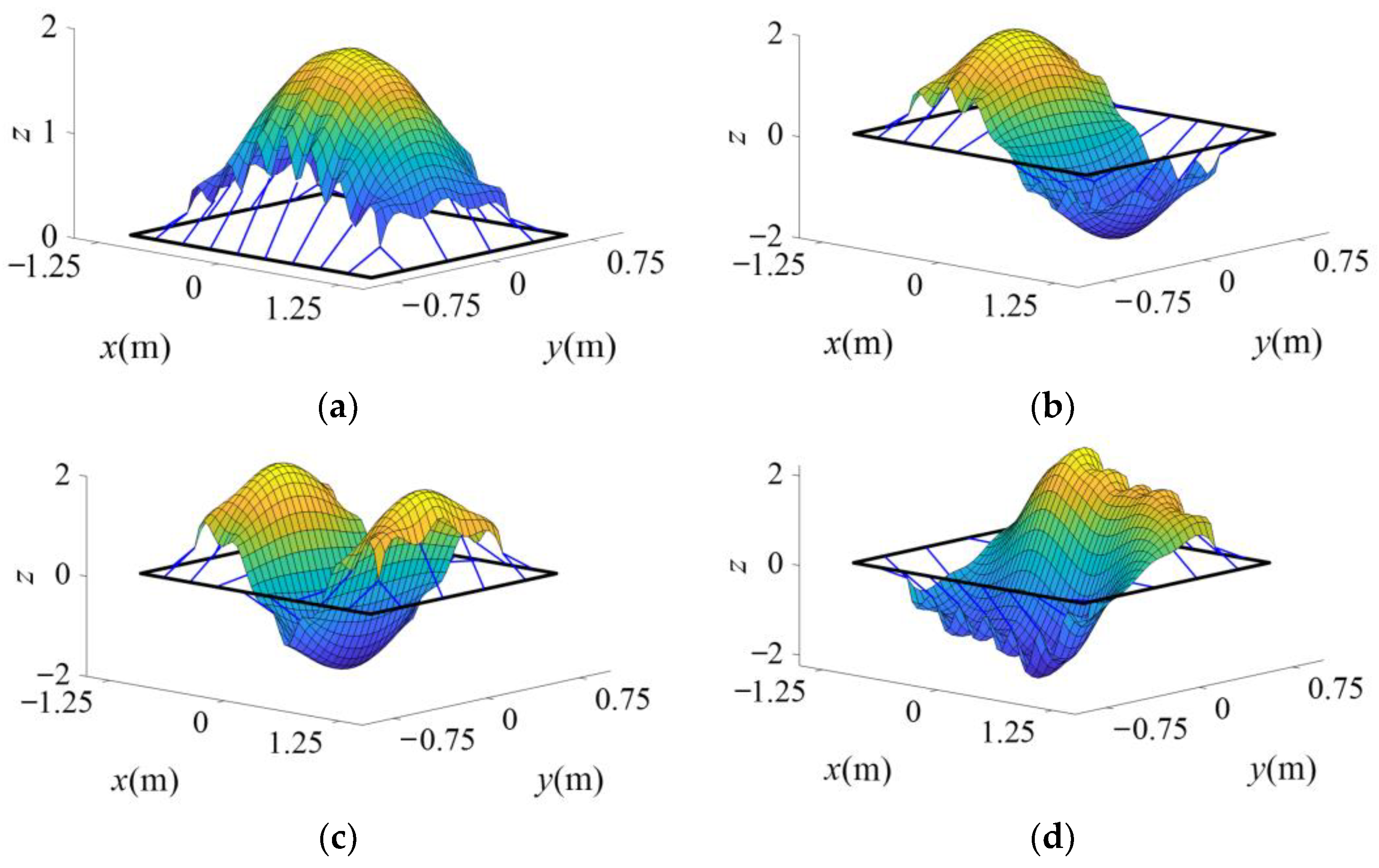
Table 1. Based on the obtained dynamic model, the natural frequencies of some modes of the membrane antenna, which are only related to the mass and stiffness of the antenna system, are shown in
Table 2, and the shapes of the first four modes are shown in
Figure 3. It should be noted that the natural frequencies are used to illustrate the basic dynamic characteristics of the membrane antenna in this section, and to make comparison with vibration frequencies to explain how the rigid–flexible coupling effect influences the response. Since the membrane antenna is a biaxially symmetrical structure, the mode shapes are symmetric or central symmetric. For the membrane antenna in this section, the first and third modes are symmetric, while the second and fourth modes are central-symmetric. Because symmetry of modes has little correlations to the research on the rigid–flexible coupling effect, emphasis will not be put on symmetry of modes in the following sections.
Assume that the antenna structure has proportional damping,
C =
αM +
βK, where
α and
β are damping coefficients. It is considered that the membrane antenna rotates at a constant angular velocity
ω0 at first, then decelerates from a certain moment, and finally comes to a standstill after a certain period of time
T. Without losing generality, an arbitrary point
A with coordinates (0.7036, 0.4267) on the membrane is selected as the measuring point, as shown in
Figure 1b. Firstly, we assume that the initial angular velocity
ω0 = π/5 rad·s
−1,
T = 1 s and
α =
β=0.01. The membrane antenna shapes at different moments are listed in
Figure 4, where the vibration displacements have been magnified 1000 times to facilitate observation. The time response of the out-of-plane displacement of point
A in this process is shown in
Figure 5a. It can be found that during the first second, when the membrane antenna is decelerating, because of the inertia, the vibration equilibrium point of point
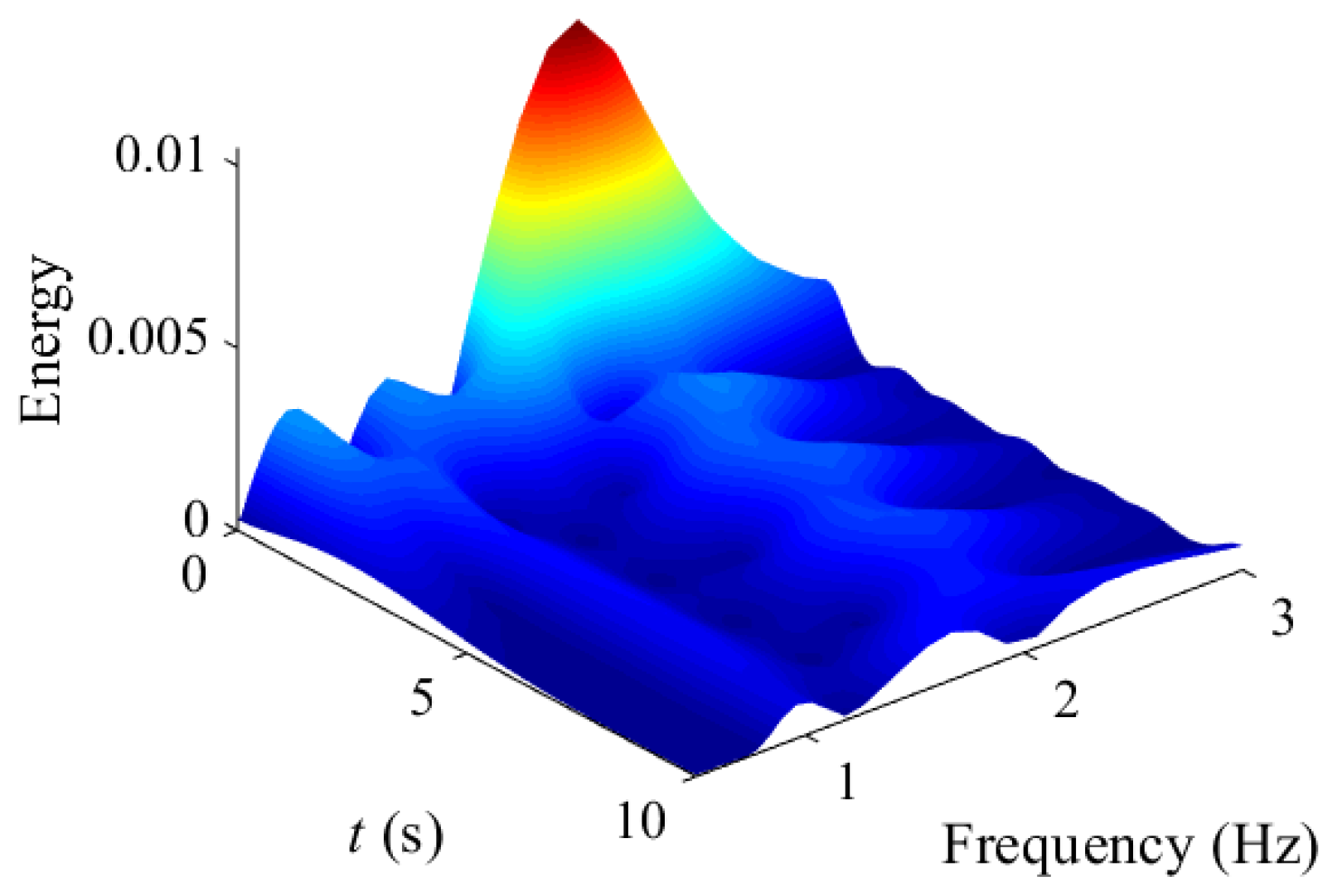
A is not located in the plane before the membrane is deformed. When the rigid body motion stops, the out-of-plane displacement is approximately symmetrical with respect to the original plane of the membrane. Due to the damping effect, the vibration of the structure decays rapidly after two seconds. The frequency characteristics changing with time can be obtain by 3D wavelet transformation, as seen in detail in
Figure 6. The frequency reaches the peak when deceleration starts because the velocity and acceleration of rigid motion contribute to the stiffness of antenna system as Equation (49) shows. The energy rises pretty high at initial and then reduces after about one second, which corresponds with the displacement response. The frequency decreases as vibration attenuates due to the nonlinearity. The energy gradually decreases as amplitude falls off, and the stable vibration frequency fluctuates around 2 Hz, eventually.
Then, in order to investigate the influence of the damping coefficients, set
α =
β = 0.001. The time response of point
A is shown in
Figure 5b. It can be found that the attenuation of structural vibration is much slower. Then, we set
ω0 = π/2 rad/s; the time response of point
A is given in
Figure 5c. It can be observed that the membrane vibration amplitude increases significantly as the initial kinetic energy increases. Moreover, the vibration of the structure has no obvious attenuation during the first ten seconds.
A series of displacement response vectors
Xi can be obtained with a full-order finite element analysis employed. The proper orthogonal modes (POMs), which are the most significant contribution to the nonlinear dynamic response, are identified through proper orthogonal decomposition (POD). A set of normal modes resembling desired POMs are selected according to the modal assurance criterion. Therefore, the modal analysis of the dominant shape obtained by numerical simulation is then carried out [
26].
The response vectors
Xis are stored at discrete output times in the so-called snapshot matrix
X. A correlation matrix
R could be obtained from snapshots matrix as
where
n is the number of output time samples and
N is the number of degree of freedoms. The eigen analysis is then performed on correlation matrix
where
λ and
p are eigenvalue and eigenvector, respectively. As in normal mode analysis, eigenvectors can illustrate the mode shape in a response, which is called a proper orthogonal mode (POM), while eigenvalues indicate the significance of their corresponding shape, which is called proper orthogonal value (POV). The larger the POV is, the more contributions the corresponding POM has made. The participation of POM can be determined by participation factor
χi, which is
The sum of all participation factors should be 1. When selecting POMs with a number of
M (
M <
N), the cumulative participation factors of selected POMs can be expressed as
The POMs could resemble normal modes a lot for simple structures, while they could be quite different for complex structures with high DOFs such as membrane antenna. The modal assurance criterion (MAC) is therefore applied to measure the similarity of a pair of POM and normal mode [
27]. The MAC value of a pair of vectors could be written as
where
pk is one of select POMs and
φl is one of normal modes. Normal modes are sorted by their MAC values, and
M could be adjusted according to the cumulative participation factor.
The combined shape of POMs with a participation factor of 99% of the membrane antenna is shown in
Figure 7, which is a so-called dominant shape.
Table 3 offers five normal modes with the highest MAC values and their cumulative participation factor.
It can be seen from
Table 3 that the dominant mode of the membrane antenna is similar to its fourth-order mode with a similarity as high as 76.28%. Therefore, it can be considered that its mode shape is dominated by the fourth-order mode shape. However, compared with
Table 2, one can find that the response frequency of the membrane antenna in
Figure 5 is larger than its fourth-order frequency. This indicates that under the disturbance of rigid body motion, the dynamic response frequency of the membrane antenna is not consistent with its modal frequency of the corresponding order mode shape. The dominant mode shape is related to its rigid body motion, while its dynamic response frequency is affected by both the structure itself as well as the rigid body motion. In
Section 4, we will discuss the influence of the rigid body motion on the dynamic response characteristics of the membrane antenna through multiple sets of numerical examples.
4. Discussion on Rigid–Flexible Coupling Nonlinear Dynamic Characteristics
In this section, four different case studies are carried out to analyze the dynamic response of point
A in the time domain and frequency domain, and to discuss the influence of rigid body motion (acceleration, initial velocity and deceleration duration) and structural fundamental frequency on the rigid–flexible coupling dynamic response characteristics under the disturbance of antenna attitude adjustment. Three membrane antenna models of different fundamental frequencies are first obtained by adjusting the pretension forces of the cables, which are named M1, M2 and M3. The influences of the initial rotational velocity
ω0, the deceleration duration
T and the corresponding acceleration on the dynamic response of three models are discussed, respectively. The frequency components of antenna vibration are extracted by FFT. Though the frequency is varying for a nonlinear vibration, the distribution of frequency components is kind of concentrated. The frequency component with highest energy was, therefore, selected to represent the frequency characteristic of the vibration. The fundamental frequencies of three models and the corresponding pretension forces are listed in
Table 4. The parameters of rigid body motion used in the case studies are shown in
Table 5.
Firstly, the dynamic responses of different models with the same rigid body motion are analyzed. The initial rotational velocity
ω0 = π/100 (rad/s), the deceleration duration
T = 0.1 s. The time histories of point
A are shown in
Figure 8 and the dynamic response frequencies and amplitudes are shown in
Table 6. It can be observed that under the same rigid body motion, the dynamic response frequency of the membrane antenna is positively correlated with the fundamental frequency of the structure, while the maximum amplitude is negatively correlated with the fundamental frequency of the structure.
Then, the dynamic responses of model M3 with the same initial rotational velocity
ω0 but different deceleration duration
T are discussed. Assume that
ω0 = π/5 (rad/s),
T = 0.1 s, 1 s and 2 s, the time histories of point
A are shown in
Figure 9 and the dynamic response frequencies and amplitudes are shown in
Table 7. One can find that with the increase of
T, the response frequency and amplitude decrease, and the nonlinearity of the system becomes obvious. It also shows that the inertia force creates a new balanced position for nodes of the membrane antenna, instead of the plane before maneuvering. This is the reason why the displacement of A keeps positive before rigid motion stops.
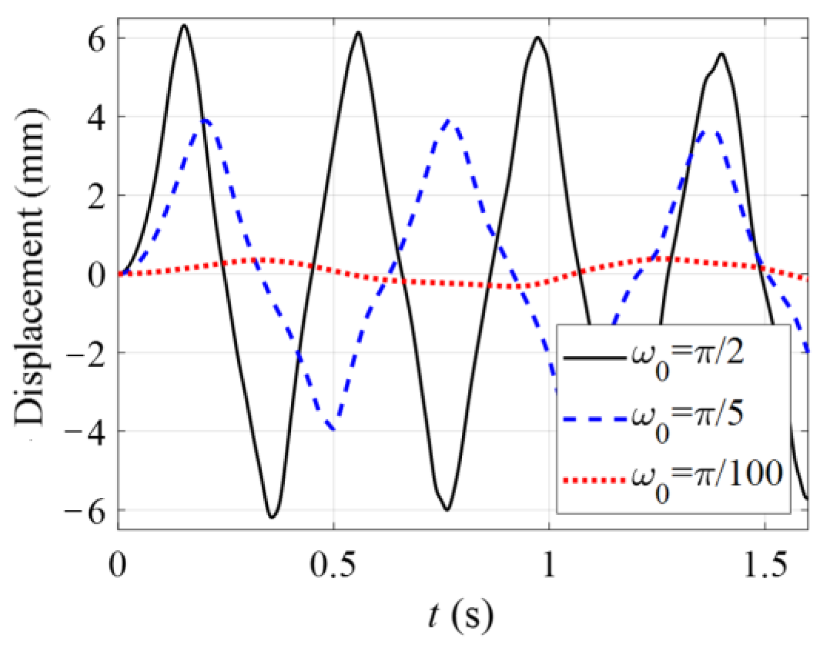
Next, the dynamic responses of model M1 with different initial rotational velocity
ω0 but the same deceleration duration
T are discussed. Assume that
ω0 = π/2 (rad/s), π/5 (rad/s) and π/100 (rad/s), the deceleration duration
T = 0.1 s. The time histories of point
A of the three cases are shown in
Figure 9 and the dynamic response frequencies and amplitudes are shown in
Table 8. It is obvious that the response frequency decreases with the decrease of initial rotational velocity
ω0. Additionally, the vibration amplitude evidently declines with the decrease of
ω0. From the discussion above we can draw the following conclusion: (1) the response frequency and vibration amplitude of the membrane antenna is strongly influenced by acceleration of the rigid body motion, i.e., for the same model, a larger acceleration will lead to a higher response frequency and a larger vibration amplitude; (2) the energy of vibration is dominated by the initial kinetic energy of the membrane antenna, i.e., for the same model, a larger initial rotational velocity will contribute to a larger vibration amplitude.
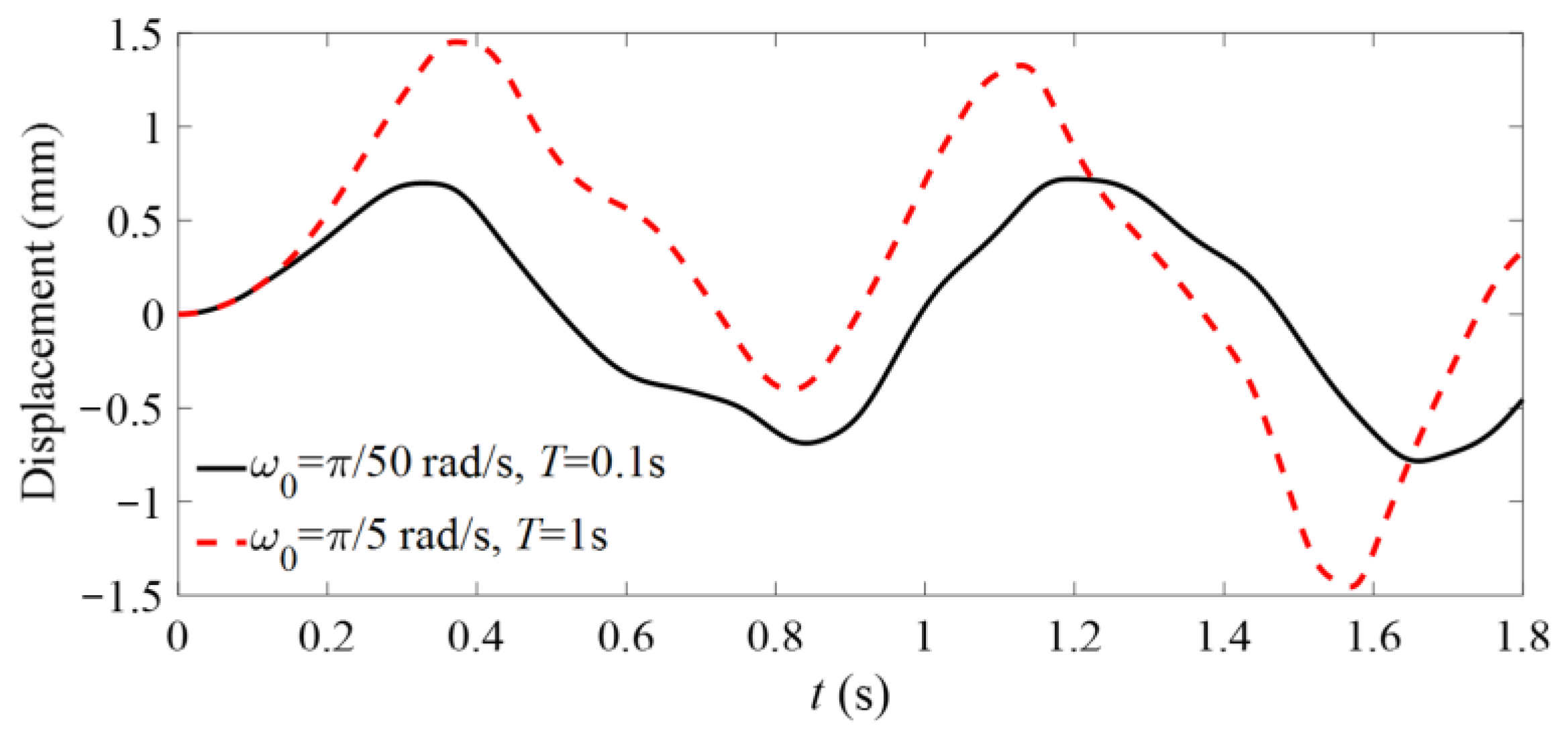
In
Figure 10 and
Table 8, the influence of initial velocity and deceleration duration have been discussed. We assume that the antenna rotates with the same initial velocity but different deceleration duration, or with different initial velocity but the same deceleration duration. However, there is another case that needs to be discussed, i.e., the antenna rotates with different initial velocity and different deceleration duration, but the same acceleration. Assume that the membrane antenna rotates in the following two cases: (1)
ω0 = π/5 (rad/s),
T = 1 s; (2)
ω0 = π/50 (rad/s),
T = 0.1 s. The time histories of point
A are shown in
Figure 11 and the dynamic response frequencies and amplitudes are shown in
Table 9.
From
Table 9, one can find that although the accelerations of the two cases are the same, the dynamic responses are still different. The amplitude and response frequency are larger when the initial rotational velocity is π/5 (rad·s
−1). Therefore, under the condition of the same acceleration, the initial velocity has more influence on the rigid–flexible coupling response than the deceleration duration.
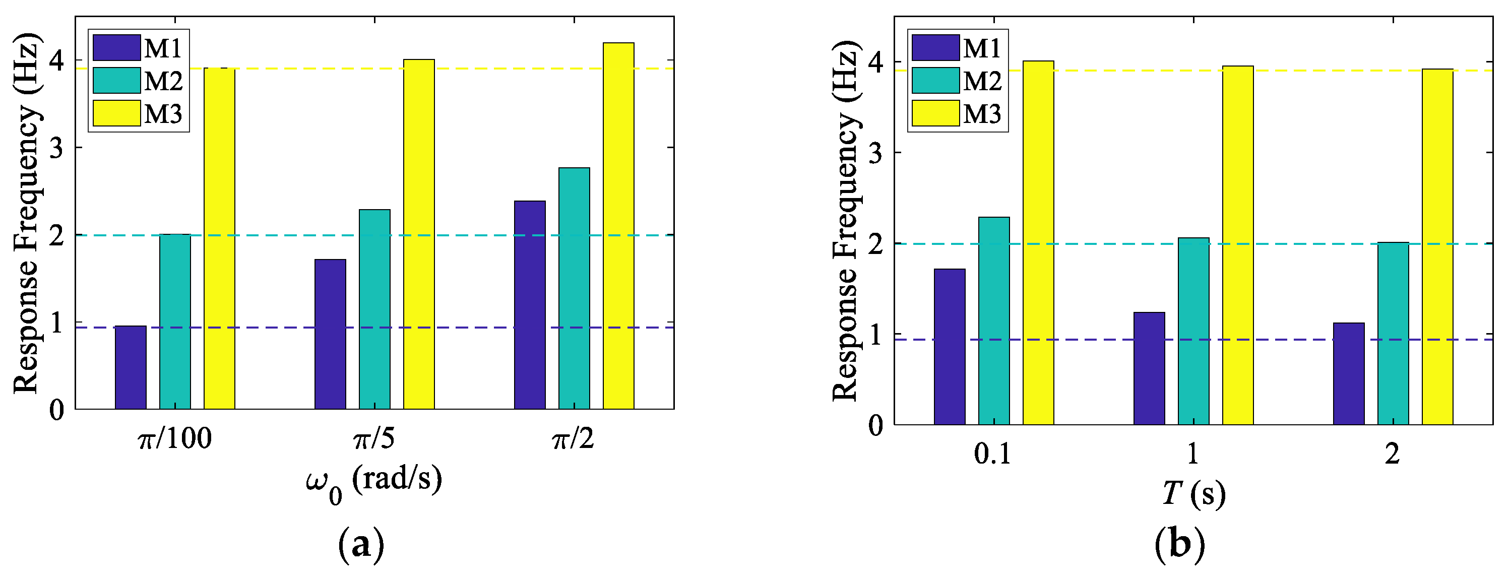
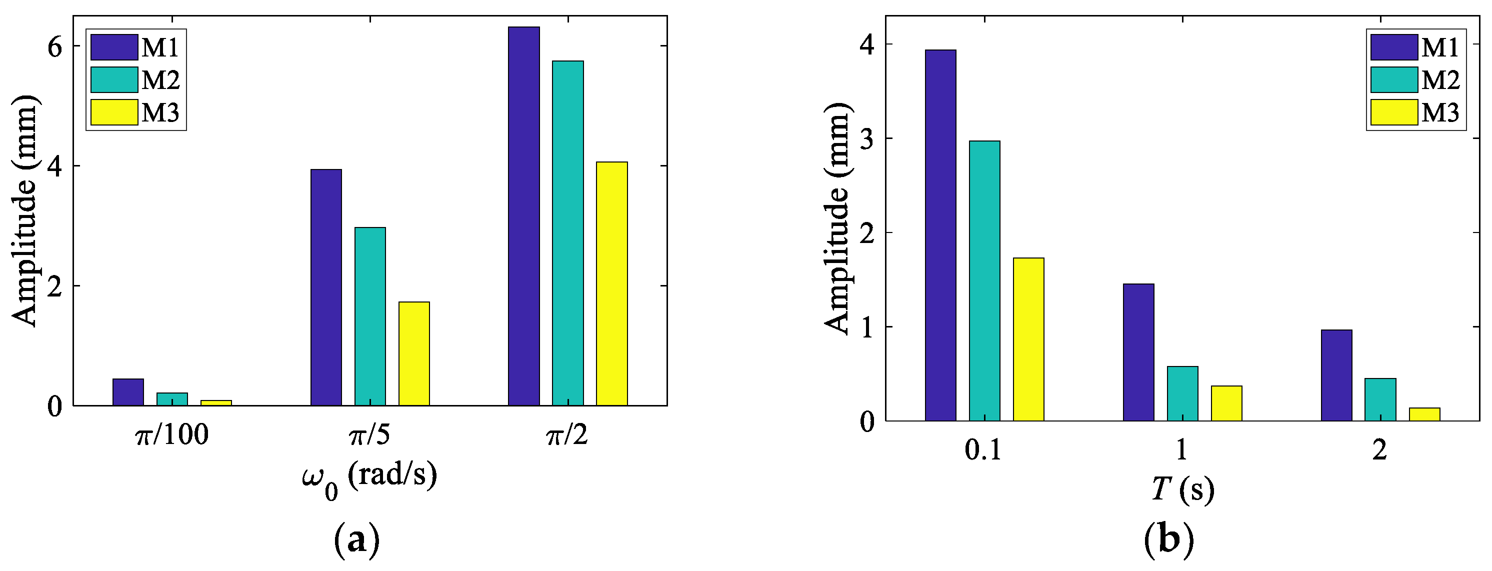
It can be seen from the above case studies that the rigid body motion has a significant influence on the dynamic response characteristics of the space membrane antenna due to the rigid–flexible coupling effect, and the influence is related to the modal characteristics of the structure. For three models M1, M2 and M3, with different fundamental frequencies, the detailed influences of rigid motion on the dynamic response of the antenna are displayed in
Figure 12 and
Figure 13.
The blue, green, and yellow dotted lines in
Figure 12 denote the natural frequencies of the dominant mode (fourth-order mode) of models M1, M2 and M3, which are 0.94 Hz, 1.99 Hz and 3.90 Hz, respectively. It can be found that the response frequency increases with the increase of the fundamental frequency of the model. At the same time, the rigid–flexible coupling response frequency of the structure climbs with the increase of the rigid body motion acceleration. When the acceleration approaches zero, the influence of the rigid–flexible coupling effect decreases significantly, and the structural response frequency approaches the natural frequency of the dominant mode. From
Figure 13, one can find that the vibration amplitude of the structure decreases with the increase of fundamental frequency and deceleration duration, and increases with the increasing of initial velocity. Comparatively speaking, the initial kinetic energy of the structure dominantly determines the maximum vibration amplitude that could be achieved. In addition, by comparing the three models, the response frequency of M1 is significantly affected by the initial velocity and deceleration duration, while the influence on M3 is relatively weak. This means that under the same rigid body motion condition, the rigid–flexible coupling effect will have a stronger influence on the structure with lower fundamental frequency.


