Article

Fluid–Structure Interaction Dynamic Response of Rocket Fairing in Falling Phase

1
School of Aeronautic Science and Engineering, Beihang University, Beijing 100191, China
2
Beijing Institute of Astronautical Systems Engineering, China Academy of Launch Vehicle Technology, Beijing 100076, China
*
Author to whom correspondence should be addressed.
Aerospace 2022, 9(12), 741; https://doi.org/10.3390/aerospace9120741
Submission received: 28 September 2022 / Revised: 19 November 2022 / Accepted: 21 November 2022 / Published: 23 November 2022
(This article belongs to the Special Issue Structural Dynamics and Control)

Abstract

:
A method based on fluid–structure coupling is used in this study to calculate the response of a rocket fairing as it is falling. Some cases of vibration divergence of the fairing were found, and the influence of some specific factors was analyzed. The aerodynamic forces are calculated by using computational fluid dynamics (CFD) software and the structural responses by the modal-superposition method. The data are then subjected to modal interpolation in the CFD solver for the next cycle of calculation. The dynamic pressure, Mach number, and angle of attack are fixed in this process. Given that the fairing has a fixed attitude during falling, its rotation is ignored in calculations for the simulation. The results are then used to propose a framework for the fluid–structure coupling-based analysis of a non-streamlined structure. The mechanism of the fairing is discussed based on this method, and the effects of the settings of the solver, Mach number, dynamic pressure, and structural stiffness on it are investigated. Dangerous and safe regions are identified as the fairing falls back to the ground. Three methods are then provided based on the above analysis to prevent damage to the fairing as it falls to ground, such as increasing structure rigidity, attitude control, and opening the parachute at high altitude. A comprehensive method was used to suppress the vibration of the fairing during the descent, which was proven to be effective.

1. Introduction

The fairing of a rocket is expensive, and accounts for a large part of the cost of launching. When the fairing is separated from the rocket at a high altitude, it falls back to the ground along with the remaining wreckage. This poses a safety hazard, and the fact that the fairing cannot be reused significantly increases the cost of the rocket. Figure 1 shows typical fairings. Recycling and reusing the fairing is a popular subject of investigation in commercial aerospace research and a new scheme for recovering the fairing has been proposed here. Following launch, the fairing detaches from the rocket as the air thins high in the atmosphere. A parachute is used to ease its fall as the fairing speed slows to subsonic speed and it is recovered when it reaches the ground. As the flexible shell of the fairing falls at a high speed, it is subjected to complex fluid–solid coupling under the action of airflow before the parachute opens, and thus may suffer damage. It is important to study this complex problem of fluid–solid coupling. Analyses of the fluid–structure interaction (FSI) that induce the failure of the non-streamlined structure during its descent are carried out to prevent accidents and provide a reference for the design of the fairing.
Methods to calculate aeroelasticity in the context of aerospace research can be divided into three categories: theoretical algorithms for the frequency domain of aeroelasticity [1], methods to calculate aeroelasticity based on a reduced-order model (ROM) [2], and coupled numerical calculations using computational fluid dynamics (CFD) and computational structural dynamics (CSD) [3]. The doublet-lattice method is an example of methods of calculation in the frequency domain [4], and reduced-order aerodynamic models include the Volterra series and the radial basis neural network [5,6,7]. With advances in CFD and CSD, numerical calculations based on the theory of FSI provide novel means for dealing with problems of unsteady aeroelasticity.
Researchers in aviation have developed mature methods to analyze the streamlines of wings and aircraft. Torregrosa used the ROM method to study non-linear aeroelastic phenomena and applied the results to beams [8]. Xie established a non-linear, geometric FSI model based on the “quasi-modal” method of a non-constant vortical lattice combined with structural dynamics, and used it to examine the problem of the gust response of large-scale wings with a flexible chord ratio [9]. Kenneth used numerical calculations based on CFD/CSD coupling to simulate the movement of a two-dimensional wing with gaps and analyzed its flutter characteristics. This work formed the foundation for the subsequent investigation of problems of aeroelasticity [10]. Hallissy and Cesnik developed a highly precise tool for the aeroelastic simulations of flexible wings through weak CFD/CSD coupling [11]. To study the linear and non-linear static aeroelasticity of flexible wings, Mian developed a numerical method that weakly couples an open-source structural dynamics software with the Reynolds-averaged Navier–Stokes (RANS) equations. The results of calculations of the model of an aeroelastic wing by using this method were in good agreement with experimental data [12]. Ilie developed a time-domain numerical model based on bidirectional CFD/CSD coupling to simulate aeroelastic responses of helicopter blades [13]. Aprovitola focused on the static pitching stability of the aircraft to examine the effects of variations in the Mach number on the shift in its aerodynamic center by using both a commercial (ANSYS-Fluent) tool and an open-source (SU2) code [14]. Franzmann used an experimental method to measure the coefficient of the damping moment of the pitch of a rocket at a certain angle of attack and obtained results that were consistent with those of CFD simulations [15]. Zhong studied a control system that can reliably separate the fairing under a high dynamic pressure and suppress interference in this process [16]. Seiji used a hybrid LES/RANS-based method to simulate the transonic flow-field around a rocket fairing [17].
However, research on the fairing of the rocket has mainly focused on its acoustics and shape [18,19,20], and no references were found which studied issues of the rocket fairing recycling for engineering applications. The traditional doublet-lattice method cannot be applied to develop a flexible and non-streamlined configuration of the fairing. A CFD–CSD coupling method is required. Due to the lack of research on this object, the design department lacks cognition of influences of relevant paraments. It is worthwhile to study this problem.
In this paper, the motion of the fairing as it falls before the parachute opens is studied. Firstly, a framework for fluid–structure coupling-based analysis is proposed, which is based on CFD and the modal-superposition method to investigate the non-streamlined configuration of the rocket fairing and provide a dynamic response analysis for it reuse [21,22]. Unsteady aerodynamic forces and the structural response are calculated by a CFD software and the modal-superposition method. Data on the displacement are passed to the CFD solver through interpolation calculation for the next round of calculations. Then, simulations of the typical cylindrical vortex-induced vibrations that are consistent with past work are performed to verify the effectiveness of the proposed method. Furthermore, the dynamic response analysis in the recycling process of fairing is analyzed [23]. Typical working conditions are selected during the calculations to observe the stability of the response of the fairing while maintaining a constant dynamic pressure, Mach number, and angle of attack. The rotation of the fairing is ignored in the calculations. The influences of Mach number and dynamic pressure are discussed, and dangerous and safe regions for the descent of the fairing are identified. Three methods are then provided based on the above analysis to prevent damage to the fairing.

2. Basic Theories of FSI

Due to uncertainty in the movement of the fairing as it falls and limitations on its size, it is difficult to conduct wind tunnel tests. The motions of fluids and structures are often complex. Aerodynamic forces deform the structure of the fairing, and the displacement generated by its deformation changes the shape of fluids which cause structure deformation. The interaction between the fluid and the solid renders the problem unsteady in the time domain. Numerical methods are used to study this problem, which involve modeling the fluids and the structure as well as accurately calculating their responses and interactions.
The panel method is widely used to calculate the aerodynamic force due to its convenience of use, but it is not suitable for problems involving large deformation and non-linearity. Reduced-order models have received increasing attention in recent years, but their inadequate capability of generalization and the long training time needed by them limit their application. Unsteady aerodynamic forces were calculated by using CFD to accurately study the movement and mechanism of failure of the fairing as it falls.
Since the structure of the fairing is relatively simple, its main modes over several orders can reflect structural deformations in it. The modal-superposition method was used for structural calculations with several main modes to reduce the number of requisite calculations.
The numerical solution based on CFD/CSD coupling has advantages in terms of solving problems in aerospace research. Fluid–solid weak coupling is used to solve the problem, and the data are exchanged through the interface between the fluid and the solid.
Since structural displacement cannot be ignored during the descent of the fairing, bidirectional fluid–structure coupling is needed in calculations of the simulation.

2.1. Fluid Mechanics

A method based on the RANS equation is used to study the motion of the fairing in the atmosphere. The basic control equations of the fluid include the equation of continuity and the Navier–Stokes equation. They can be integrated into the following form [24,25]:
t V W dV + V F C d S V F V d S = 0
where,
W = [ ρ ρ v ρ E ] F C = [ ρ V r ρ V v + p n ( ρ H + p ) V r + V t p ] F V = [ 0 τ ¯ n k ( T n ) + ( τ ¯ v ) n ]
In the above expressions, W represents the vector of the conservative variables, F C and F V are the vectors of convective and viscous fluxes, respectively, p , ρ , v , T , and E denote the pressure, the density, the velocity vector, the temperature, and the total energy per unit mass, respectively, V t stands for the contravariant velocity of the face of a control volume and V r represents the contravariant velocity relative to the motion of the grid, n refers to the outward-facing unit normal vector of dS , k is the thermal conductivity coefficient, and τ ¯ is the viscous stress tensor.

2.2. Basic Theory of Structural Dynamics

FSI was used to study the motion of the fairing during recovery. The equation of an n degree of freedom (DOF)-damped system’s forced vibration in the z direction is:
M z ¨ + C z ˙ + K z = f
where z represents the vector formed by displacement of n degrees of freedom along the vibration direction, M , C , and K denote the mass matrix, damping matrix, and stiffness matrix, respectively, and f represents the load.
The natural modes of the model are ϕ 1 ( n × 1 )   ~   ϕ n ( n × 1 ) , and can be written as the following matrix:
ϕ 1 ( n × 1 )   ~   ϕ n ( n × 1 )
Multiplying the left side of Equation (3) by Φ T yields:
Φ T M z ¨ + Φ T C z ˙ + Φ T K z = Φ T f
The displacement vector z can be represented by the generalized displacement q corresponding to the mode of each order:
z = Φ q = i = 1 n ϕ i q i
Φ T M Φ q ¨ + Φ T C Φ q ˙ + Φ T K Φ q = Φ T f
When the mode of each order is a mass-normalized mode, the damping matrix is ignored:
I q ¨ + C p q ˙ + Ω q = Φ T f
where I ( n × n ) is the identity matrix, C p ( n × n ) = d i a g ( 2 ζ i ω i ) is a diagonal matrix, and Ω ( n × n ) = d i a g ( ω i 2 ) is also a diagonal matrix. M p = Φ T M Φ represents the generalized mass matrix, and ζ is the damping ratio. When Φ consists of mass-normalized modes, M p is equal to I , C p = Φ T C Φ represents the generalized damping matrix, K p = Φ T K Φ represents the generalized stiffness matrix, and K p is equal to Ω .
Generalized forces are involved in the calculation process. The program firstly reads the pressure of every aerodynamic grid at each time step, and then calculates the aerodynamic force of each aerodynamic grid. In the same time step, the mode shapes of the aerodynamic center are obtained from locations of nodes of the structure model and the mode shapes of the structure model through the Thin-Plate Spline (TPS) interpolation algorithm. The aerodynamic force is multiplied by the mode shape, and then by its area to obtain the generalized force for each aerodynamic mesh.
The generalized force is defined as:
F = ϕ i p i S i
After the generalized aerodynamic force is obtained, it is substituted into Equation (8). Then, the generalized displacement is solved by the Runge–Kuta method. After the generalized displacement force is obtained, the modal-superposition method is used to solve the physical displacement of each node. Finally, the mesh in the CFD solver completes the deformation.

2.3. Thin-Plate Spline Interpolation Algorithm

When the modal method is used to deal with the problem of FSI, it usually involves using the grids of different nodes in the regions of the fluid and the solid. The modes at nodes of the fluid mesh are calculated by the TPS interpolation algorithm. A generalized dynamic equation is established at the central node of the grid and is solved to obtain the generalized displacement and generalized velocity. The nodal displacement of the boundary of FSI is obtained by modal value interpolation, and changes according to the generalized displacement once the motion of the fluid has been solved.
The TPS interpolation algorithm can be described by the following equation:
{ c i 1 = x i c i 2 = y i c i 3 = z i } , i [ 1 p ] C p × 3 = [ x 1 y 1 z 1 x 2 y 2 z 2 x p y p z p ]
where p is the number of control points and c i ( x i , y i , z i ) , i = 1 , 2 , , p represents their location.
The regularization parameter, λ , can then be obtained, and the unknown TPS weights w and a in the linear system of equations need to be solved.
[ W P P T O ] [ w 2 a 2 ] = [ v o ] L ( p + 3 ) × ( p + 3 ) x 2 ( p + 3 ) = b ( p + 3 )
where W , P , and O are submatrices, and w , a , v , and o are column vectors that are given by the following equations:
W i j = U ( | | c i 1 c i 2 | | c j 1 c j 2 | | ) + I i j α 2 λ i , j [ 1 p ] λ 0
U ( r ) = { r 2 log r r > 0 0 r = 0
α = 1 p 2 i p j p ( | | c i 1 c i 2 | | c j 1 c j 2 | | )
P p × 3 = [ 1 c 11 c 12 1 c 21 c 22 1 1 c p 1 c p 1 ] , O 3 × 3 = [ 0 0 0 0 0 0 0 0 0 ]
P T i j = P i j i [ 1 p ] j [ 1 3 ]
v p × 1 = [ c 13 c 23 c p 3 ] , o 3 × 1 = [ 0 0 0 ] w p × 1 = [ w 1 w 2 w p ] , a 2 3 × 1 = [ a 1 a 2 w p ]
The value of z at any point can be interpolated by the following equation:
z ˜ ( x , y ) = a 1 + a 2 x + a 3 y + i = 1 p w i U ( | | c i 1 c i 2 | | x y | | )
The generalized displacement of the fairing is analyzed to determine whether the vibrations are divergent.

2.4. Dynamic Mesh

Since structural deformation occurs in the process of fluid–structure coupling, many methods are available to update the mesh. Spring smoothing is used here to adjust the mesh to represent its deformation.
For fluid regions with triangular or quadrilateral meshes, an elastic deformation-based method of mesh adjustment can be used to smoothly adjust the positions of nodes in the domain of flow. This method can smoothly adjust the volume of mesh without changing the connectivity between meshes. The connection between any pair of nodes on the grid is idealized as springs connected to each other. A boundary node moves according to a given displacement, and causes all springs connected to this node to generate a force proportional to the displacement. In this way, the displacement of the nodes on the boundary is propagated through the volume of mesh in the fluid. From the perspective of balance, the resultant force of all springs at each node must be zero. This condition can be expressed by the following iterative equation:
Δ x m + 1 i = j n i k i j Δ x m j j n i k i j
where Δ x i is the displacement of the node, m is the number of iterations, n i is the number of nodes adjacent to node i , and k i j is the spring constant between the given node and adjacent nodes, where the spring constant can be defined as:
k i j = k f a c | x i x j |
where k f a c is the spring constant factor.
Since the displacement along the boundary is known, the equation is solved for sweeping all nodes inside the fluid domain through a Jacobi matrix. During the solution process, the updated positions of the node can be expressed as:
x i n + 1 = x i n + Δ x i k , c o n v e r g e d

2.5. CFD–CSD Coupling
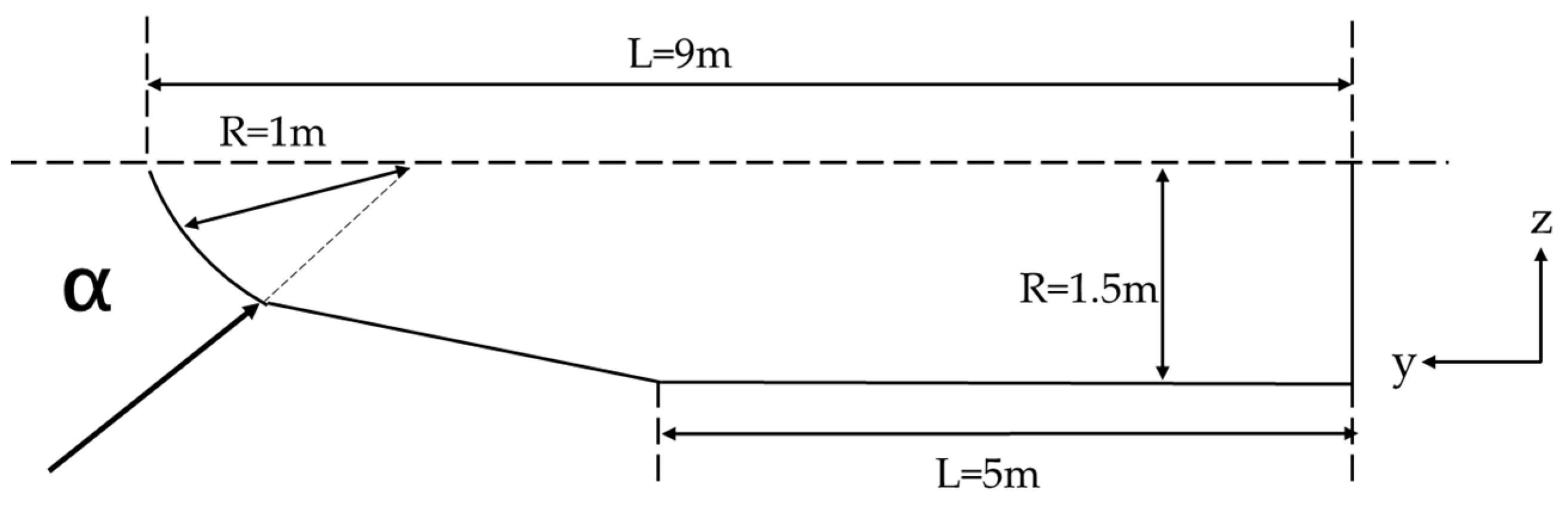
Figure 2 shows a weak coupling strategy to integrate the CFD and CSD methods.
The CFD method outputs the pressure at each moment, and then calculates the aerodynamic force at each aerodynamic face of the fairing. The mode shapes of the centers of the aerodynamic faces are obtained by using the TPS interpolation algorithm based on the locations of the structural nodes. The mode shapes are multiplied by the aerodynamic forces to obtain the generalized forces for each aerodynamic mesh. The generalized displacement is then obtained by using the generalized force in the fourth-order Runge–Kuta method to solve the equation of structural dynamics. The generalized displacement is multiplied by the mode shape to obtain the deformation of the mesh. Curves of the temporal response of the generalized force and the generalized displacement can be obtained by repeating the above process at each time step.

3. Research Object

3.1. Research Object and Working Conditions

Figure 3 shows the shape of the rocket fairing and provides the definitions of the coordinate and the angle of attack. The radius of the shell was approximately 1.5 m, the radius of the head was approximately 1 m, the length of the shell was 5 m, and the length of the fairing was 9 m. The head and fuselage were made of different materials. Table 1 lists the materials of each part of the fairing and their properties.
According to the typical state of a falling fairing, the Mach numbers M a = 0.6 and M a = 0.5 were selected as the typical working conditions for detailed calculation and analysis. The Mach number ranged from 0.2 to 0.85, and five values of the angle of attack were considered: 0°, 20°, 45°, 70°, and 90°. The effects of dynamic pressure, Mach number, angle of attack, and other factors on vibrations induced by FSI were explored by calculating for different conditions, as shown in Table 2.

3.2. Grid for the Structure and Fluid

The fairing of the rocket was modeled by shells with stiffeners. Figure 4 shows a schematic diagram of the structural grid, and the red star in it represents the displacement-monitoring point.
A modal analysis of the above structure was carried out. The first four modes were selected, which may cause failure owing to structural vibrations. The first-order mode was the torsional mode, and the second-order mode was the breathing mode. Figure 5 shows the mode shapes and the frequencies of the fourth mode. The analysis yielded vibrational frequencies of the fourth-order modes of 2.2, 5.8, 9.1, and 11.5 Hz.
The coordinate system of the CFD model was consistent with that of the structural model. The area of fluid calculation was a spherical area around the fairing with a radius of 50 m. The spherical surface of the calculation area was set as the far-field boundary, and surface of FSI of the fairing was set as the boundary of the wall. The computational grids were tetrahedral mesh. The surface meshes of the fairing were triangular elements, and the total number of meshes was 1.88 million. The mesh was refined in the area near the fairing to better capture the flow-field details in the areas near the wall and in the wake area of the fairing, with drastic changes in velocity and pressure. A schematic diagram of the grid is presented in Figure 6.
The CFD solver was Ansys Fluent and generalized displacement was calculated by the modal-superposition method, which has been mentioned in Section 2.2. The modal-superposition method is a self-programmed C language program in UDF. The first four modes were selected for the response calculation with a time step of 0.005 s and a turbulence model of k ω S S T .

4. Verification of Methods

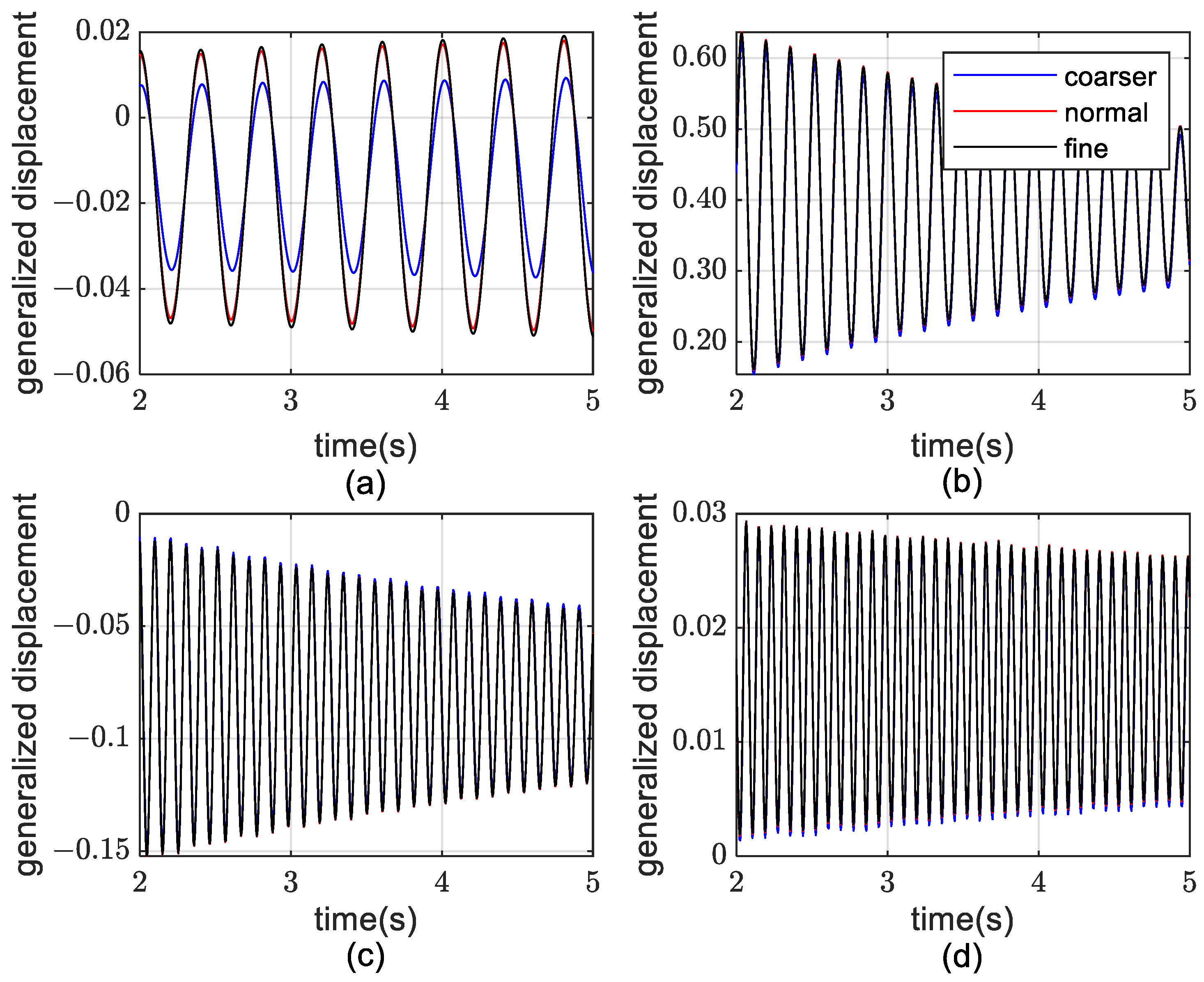
4.1. Grid Independence

The above model of the fairing was used with a Mach number of M a = 0.6 , dynamic pressure of p ¯ = 800   Pa , and angle of attack of α = 90 ° . Figure 7 compares the generalized displacement of three grid systems. Their number of grid elements and minimum volume are listed in Table 3. The mesh number was changed by adjusting the number of nodes in the circumferential and y directions on the fairing surface. In this process, the number of meshes in the inner spherical region is mainly adjusted to verify the influence of different grids. The results of the baseline grid and the fine grid were similar, and the amplitude of vibrations of the baseline grid was larger than that of the coarse grid. The generalized displacement was adequately captured by the baseline grid. Thus, the baseline grid system was used in subsequent calculations.

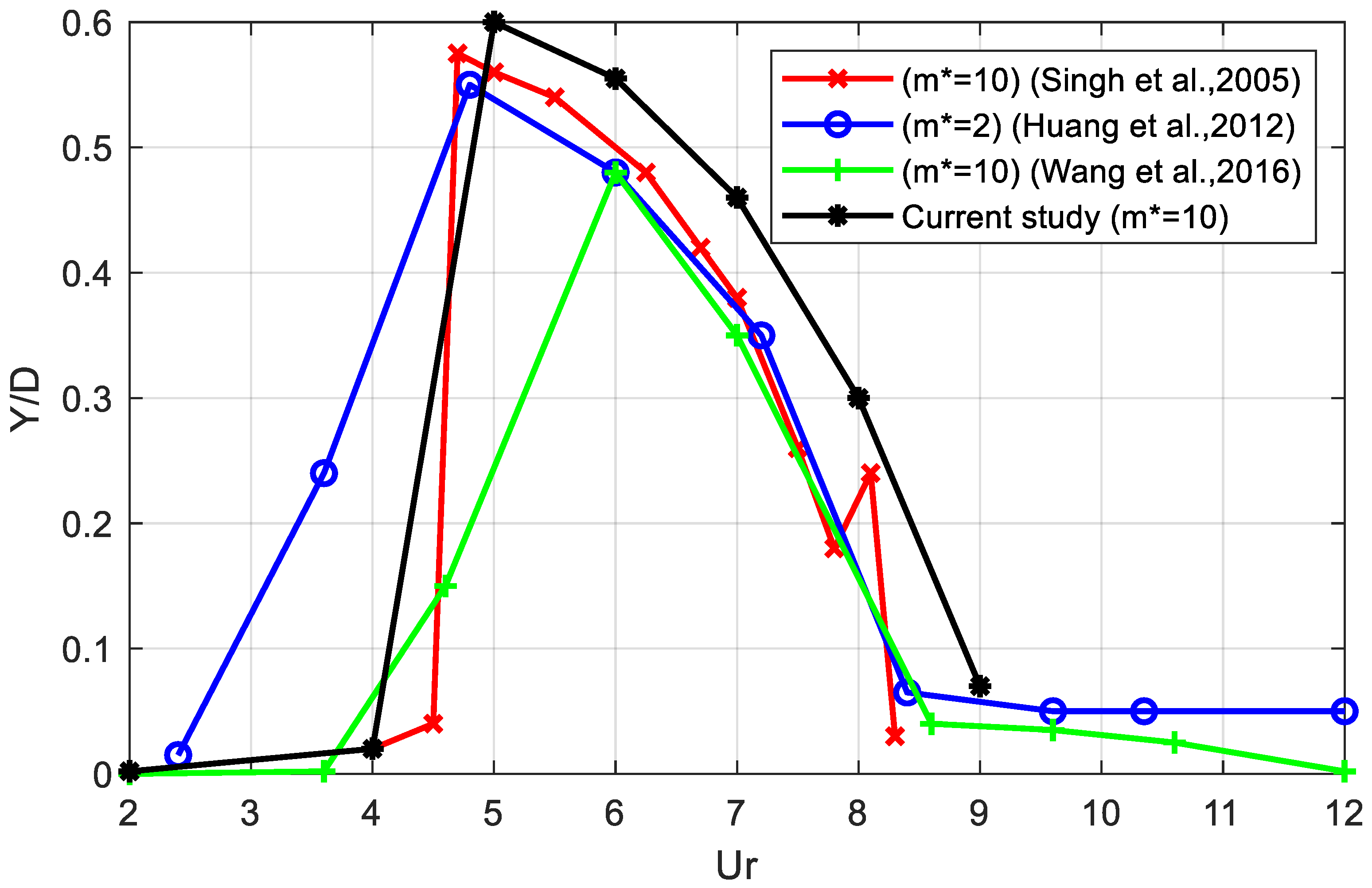
4.2. The Coupling Method

Since the object of calculation of the fairing was special, a single cylinder with a similar aerodynamic shape to the fairing was used for simulations of vortex-induced vibrations with a single degree of freedom. The aim was to verify the correctness of the method used to calculate the aerodynamic force and the deformation of the fairing under different working conditions. The result of the simulations was compared with results from past work to verify the correctness of the user-defined function (UDF) program [26,27,28]. In one time step, UDF was used to read the force from each grid and calculate the generalized force. Then, the UDF calculated the generalized displacement through the Runge–Kuta method and calculated the displacement through the modal-superposition method. Finally, the UDF updated the deformation of each node in turn. The CSD calculation was finished and the CFD solver started to run after this process.
Figure 8 shows the physical model of the vortex-induced vibrations of a single cylinder, simplified as a spring-mass-damper system. The relevant parameters were as follows: flow speed U = 0.146   m / s , flow density ρ = 1.225   kg / s , diameter D = 0.01   m , length L = 0.02   m , and kinematic viscosity μ = 1.48 × 10 6   m 2 / s . The non-dimensional mass of the cylinder was m * = 10 . To encourage high-amplitude oscillations, the structural damping coefficient was set to zero. The Reynolds number was R e = 100 and the reduced velocity was U r = 2.4 ~ 12 .
m * = m 1 4 ρ π D 2 U r = U f n D
where m is the mass of a cylinder with unit length and f n is its natural vibrational frequency.
Figure 9 shows variations in the maximum transverse displacement of the cylinder with the reduced velocity. The results of the simulation were close to those reported by Singh and Mittal [26,27,28]. Due to differences in mesh division and deformation methods, the maximum amplitude ratio was slightly higher than the reference values. However, its frequency locking range and the overall trend change were consistent. The reasons for the difference in the results of the other two articles can be found in their articles. A comparison of the variations in the maximum amplitude of the vortex-induced vibrations of a single cylinder with the reduced velocity, U r , verified the correctness of the UDF program in this paper, which was used to read the force and adjust the mesh deformation.

5. Numerical Results

To analyze the influence of the flight of the fairing as it detaches from the rocket and falls to the ground, different dynamic pressures and angles of attack, in the Mach number range of 0.2 to 0.85, were used to calculate its characteristics of FSI.
A number of cases were calculated to determine the dangerous and safe regions for the fairing as it fell and are used here to propose several methods to assess the vibrational damage to it.

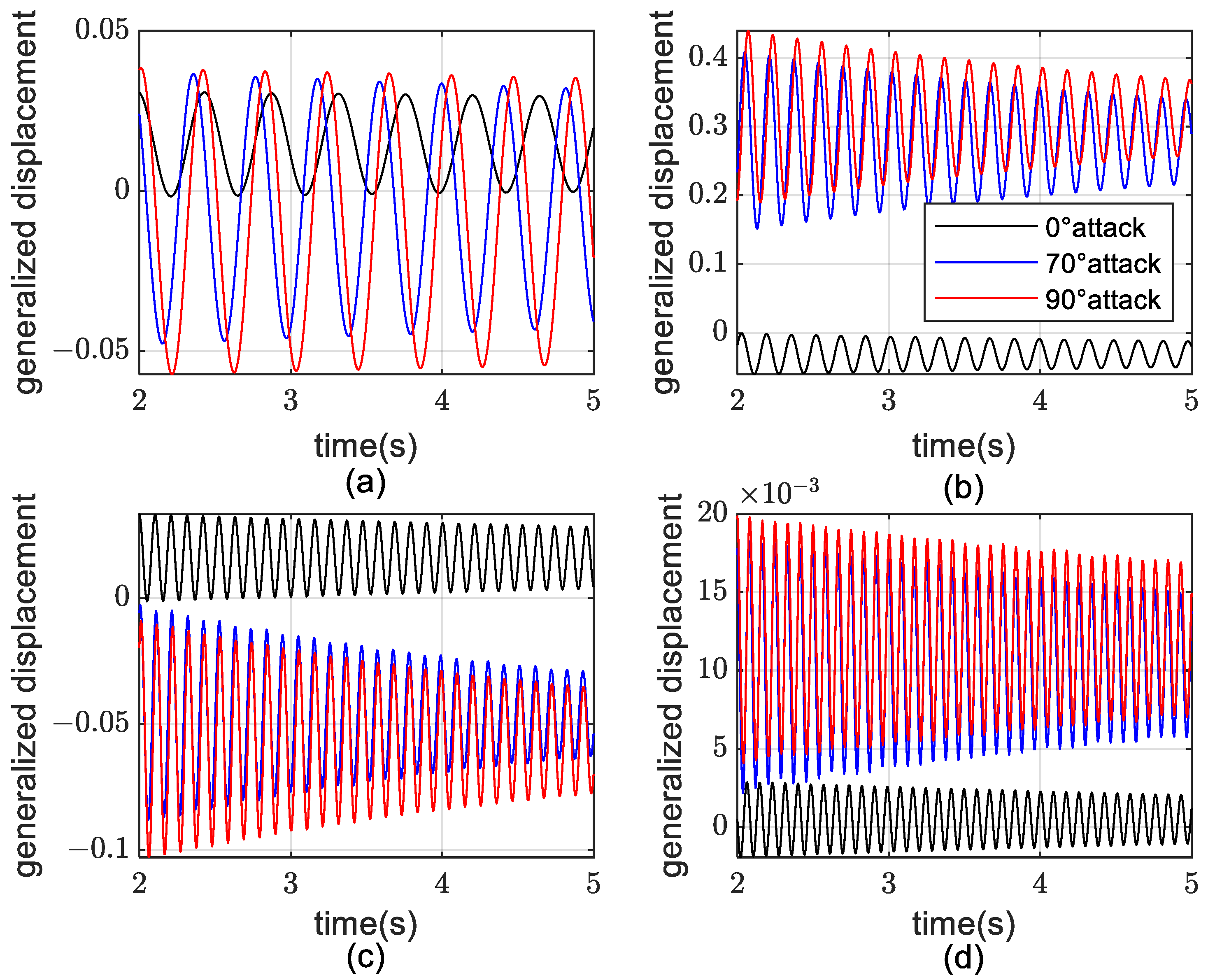
5.1. Typical Working Conditions

The structural responses of the fairing under an unsteady aerodynamic force with several angles of attack were calculated to assess its stability in different states as it fell to the ground.
Figure 10, Figure 11, Figure 12 and Figure 13 show the generalized displacement–time responses and fourth-order generalized force–time responses of the first four modes under two typical working conditions with different angles of attack ( α = 0 ° ,   70 ° ,   90 ° ).
Figure 12 shows that the generalized displacement of the fairing gradually converged when α = 0 , which shows that the vibrations were stable. When α = 70 ° , the response of the first-order generalized displacement in the time domain was close to a constant oscillation in amplitude, indicating that the structure was in a critically stable state. When α = 90 ° , the amplitude of the first-order generalized displacement gradually expanded and the vibrations of the structure diverged.
To further analyze the condition of divergence at α = 90 ° , the displacement of the monitoring point at the end of the fairing was selected to draw an image in the time domain and its power spectral density was analyzed. Figure 14 shows that the deformation diverged in the X direction, which led to the destruction of the structure. This occurred mainly due to the influences of the first-order mode.
Figure 15 shows a diagram of structural deformation in one cycle when the motion of the fairing was unstable. Due to the divergence of first-order vibrations, the torsion of the junction between the cone and the cylinder became increasingly prominent and eventually led to vibration-induced damage to the fairing.

5.2. Influence of Mach Number

Since many variables influence the working conditions, a single variable was considered for analysis. The operational dynamic pressure and the angle of attack were fixed, and a series of Mach numbers were selected for calculation. The influence of different Mach numbers on the characteristics of FSI of the fairing was analyzed and the rules of their influences were summarized. Two work conditions were considered: p ¯ = 500   Pa and α = 70 ° , and p ¯ = 700   Pa and α = 90 ° .
To discuss the stability of the generalized displacement of the fairing, the definition of its logarithmic decay rate, δ , with reference to damping was provided. Figure 16 shows the vibrational amplitude as a function of time. A value of δ greater than zero shows that the motion diverged. The larger the value of δ was, the more severe the vibrational divergence, and vice versa. The definition is as follows:
δ = ln ( x n x 0 ) n
where x n is the generalized displacement of the nth spike and x 0 is the generalized displacement at the selected initial spike.
The settings of the CFD solver were p ¯ = 600   Pa and α = 90 ° . The FSI-induced vibrations of the fairing under different Mach numbers were then calculated. Figure 17 shows that the logarithmic decay rate of the fourth-order generalized displacement continued to increase with the Mach number. In the vicinity of M a = 0.6 and M a = 0.7 , the first-order vibrations diverged, and FSI-induced failure occurred. However, as the Mach number continued to increase to around 0.8, the vibrations converged.
The operational condition of p ¯ = 800   Pa and α = 45 ° was similarly considered. Figure 18 shows that the first-order generalized displacement diverged in the Mach number range of 0.3 to 0.5. The first-order vibrations converged as the Mach number continued to increase. A comparison of the two results of the calculations shows that it is necessary to pay attention to different intervals of the Mach number in case of flutter divergence in case of first-order vibrations under different flight conditions. Since the non-linear factors are obvious in the whole calculation process, the mechanism is very complicated. According to the analysis, the primary reason for this phenomenon may be that the position and intensity of the shock wave generated on the aircraft surface are different at different angles of attack.

5.3. Influence of Dynamic Pressure

The influence of different flight pressures on the FSI-induced vibration divergences of the fairing was analyzed. Two working conditions, with M a = 0.4 and α = 45 ° , and M a = 0.6 and α = 90 ° , were selected for the calculation. Figure 19 and Figure 20 show that the problem of divergence of the first-order modal vibrations was encountered. As the dynamic pressure increased, the logarithmic decay rate corresponding to the first-order generalized displacement continued to increase, which means that the degree of divergence was more severe. The fairing was damaged due to the divergence of the first-order vibrations, which is the first-order torsional mode-induced damage of concern in this study.

5.4. Summary of the Results of Calculations

The fall of the fairing was calculated in different states, and the results were summarized. Figure 21 shows the hazard and safety zones at different angles of attack (green points represent safe states, the orange points represent the critical stable states, and the red points represent the states of structural failure).
When α = 0 , the dangerous zone was concentrated in the range of M a = 0.4 . As the angle of attack increased, this zone changed to the range of M a = 0.6 . As the angle was further increased, the zone of hazard continued to expand.

6. Improvement Methods

6.1. Increasing Structural Rigidity

An analysis of the structural displacement of the fairing shows that damage to it had been caused mainly by the first-order torsion mode. Thus, its structural stiffness was enhanced and considered to suppress the damage caused by vibrations. Given that a variety of variables affect structural stiffness and that it is inconvenient to try to control all of them, a relatively simple method of changing the thickness of the shell was chosen to change its structural stiffness.
The working condition of M a = 0.6 , p ¯ = 600   Pa , and α = 90 ° was selected for calculation and comparison. The settings of the CFD solver were the same as before.
To increase the structural rigidity, the fairing shell was thickened to 1.2, 1.5, and 1.8 times its original thickness. The mass and thickness of the shell exhibited a quadratic relationship, and its stiffness and thickness had an approximately cubic relation. The mode shapes did not change in the meantime. Taking 1.5 times the thickness as an example for illustration, the modal frequency was increased to 1.5 times that of the original, and the vibration frequencies of the fourth-order modal were 3.3, 8.7, 13.7, and 17.3 Hz, respectively. Therefore, the unit mass matrix was multiplied by the double of 1.5 and the stiffness matrix by the cube of 1.5. Other calculation parameters remained unchanged. The generalized displacement of the first-order mode was then observed to determine whether the vibrations diverged.
Figure 22 and Figure 23 show the time-dependent curves of the generalized displacement corresponding to the fourth-order mode at different thicknesses.
As the thickness of the fairing increased, the first-order vibrations gradually transitioned from divergence to convergence. This verifies that enhancing the structural stiffness can somewhat suppress vibrational divergences, where this can be used to suppress flutter.

6.2. Attitude Control

Figure 21 shows the dangerous zone of fairing, and then it is necessary to find a feasible path to safely recycle the fairing. However, the dangerous zone was not the same under different angles of attack, and it was impossible to safely land the fairing while maintaining a certain angle of attack. A strategy of controlling the angle of attack within different angles at different Mach numbers was proposed to avoid dangerous zones that can cause vibrational damage to the fairing as it falls.
SpaceX adjusts the attitude and speed of the fairings of its rockets through nitrogen propulsion and parachutes built into the fairing [29]. In this same way, the movement of the separated fairing is controlled so that it does not disintegrate. Its landing position is accurately determined at the same time.
Figure 24 shows several control schemes for the angle of attack during the process of falling of the fairing. The green and yellow lines represent the states of change of the fairing during descent. The orange dots represent its critical states and the red dots the dangerous states. However, this method encounters technical complications, such as the need for an extra control device and the complex transformation of the fairing.

6.3. Opening the Parachute at High Altitude

Normally, the parachute will open at a certain altitude. However, the fairing disintegrates before the parachute opens due to damage caused to it by the vibrations. The fairing cannot be recycled. Figure 24 shows that the damage in our simulations was mainly concentrated in the Mach number range of 0.4 to 0.7. The parachute of the fairing can be opened before its speed drops to M a = 0.7 , such that it can avoid the entire dangerous zone, and thus, disintegration.
This measure does not require complex modifications and redesign. However, the structural properties of the fairing change after the parachute opens, and this may lead to new problems related to its damage or destruction. It then becomes necessary to identify the novel states of the fairing and zones of hazard for it.

6.4. Combination of the Three Methods

Each of the above three solutions has advantages and disadvantages, which are listed in Table 4.
The effectiveness of a single method is limited. In practice, we can use a combination of different methods. To prove the validity of the method, increasing structural rigidity and attitude control were chosen to ensure the stability of the fairing during the falling process. Path one (green) in Figure 24 and 1.5 times the original thickness were considered.
Figure 25 shows the detailed situation of path one during the falling process, such as Mach number, dynamic pressure, and angle of attack. Figure 26 shows that the vibration of the first-order generalized displacement converged in the whole path. This verifies that this comprehensive method can suppress vibrational divergences and could be used to ensure the safety of the fairing in the falling process.

7. Conclusions

This study used the coupled CFD–CSD method to simulate the fall of the fairing of a rocket. The effects of the angle of attack, Mach number, and dynamic pressure during its descent were investigated. Safe and dangerous zone for it were identified during its descent, and three improvements were proposed to avoid its destruction. The conclusions of this study can be summarized as follows.
  • A framework of non-streamlined configurations with fluid–structure interactions was established. Several examples were used to verify that the proposed method can be used to calculate the FSI of the fairing and confirmed that the theoretical results corresponded to the actual situation. The work here provides ideas for future research on FSI involving objects with similar non-streamlined configurations.
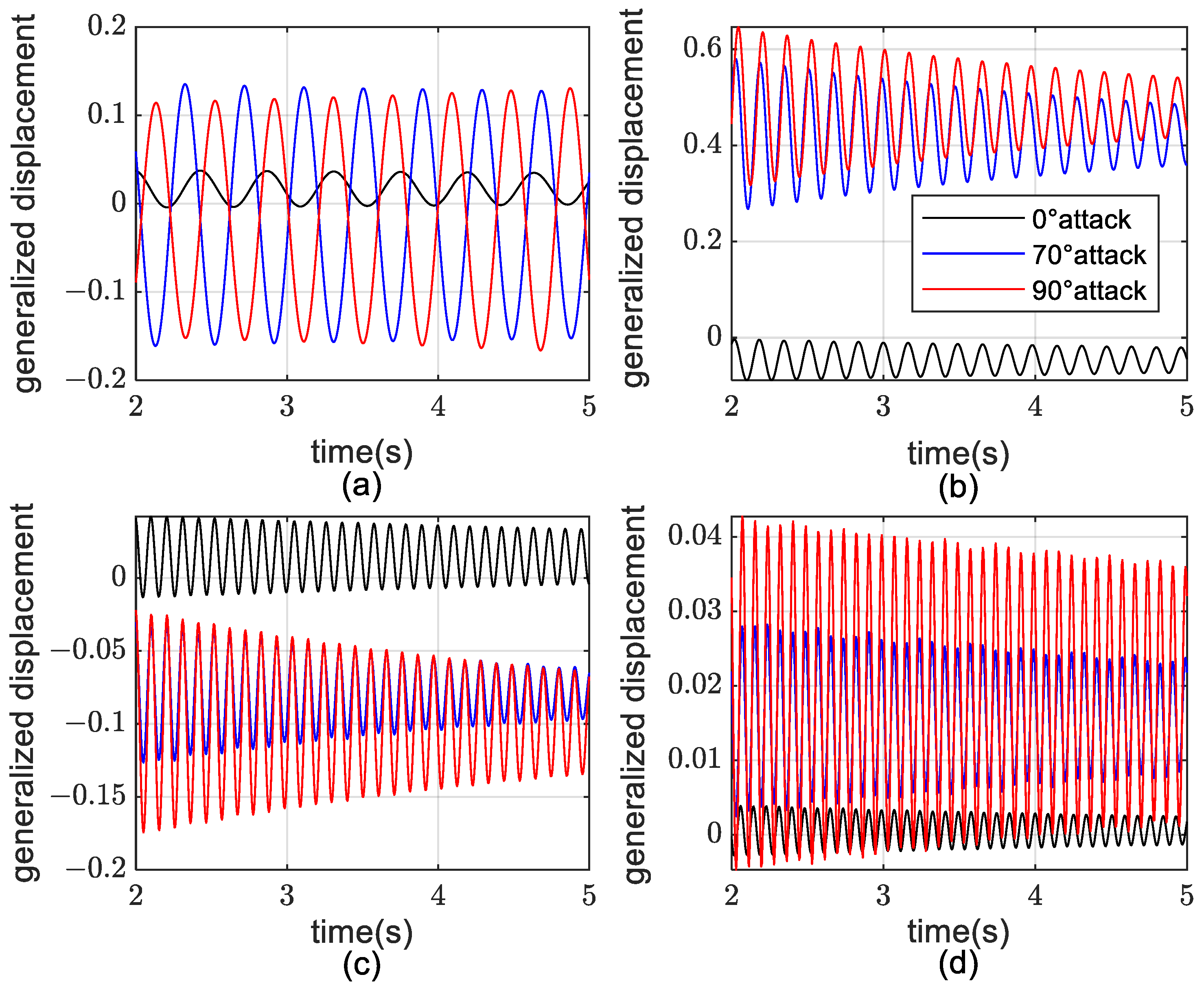
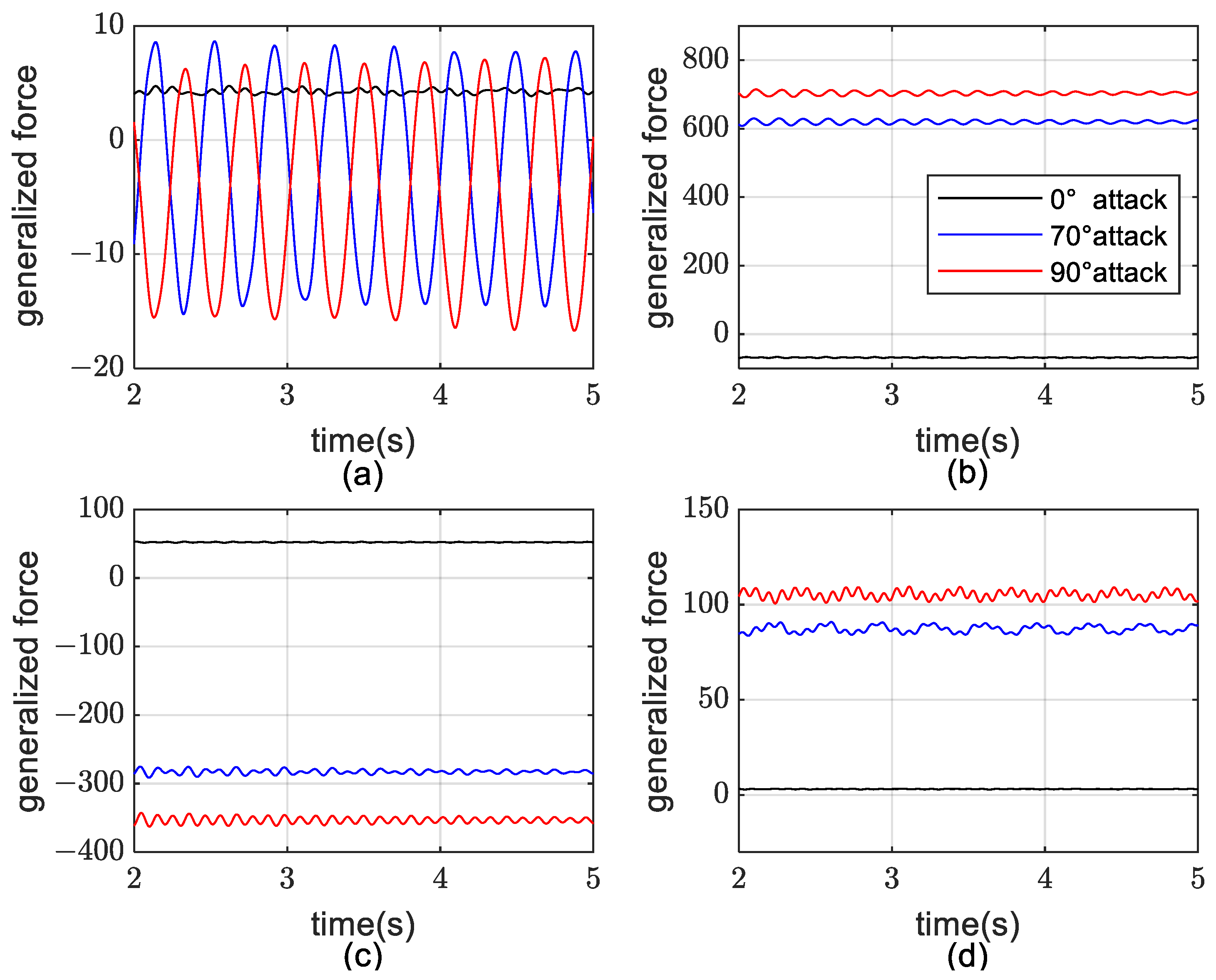
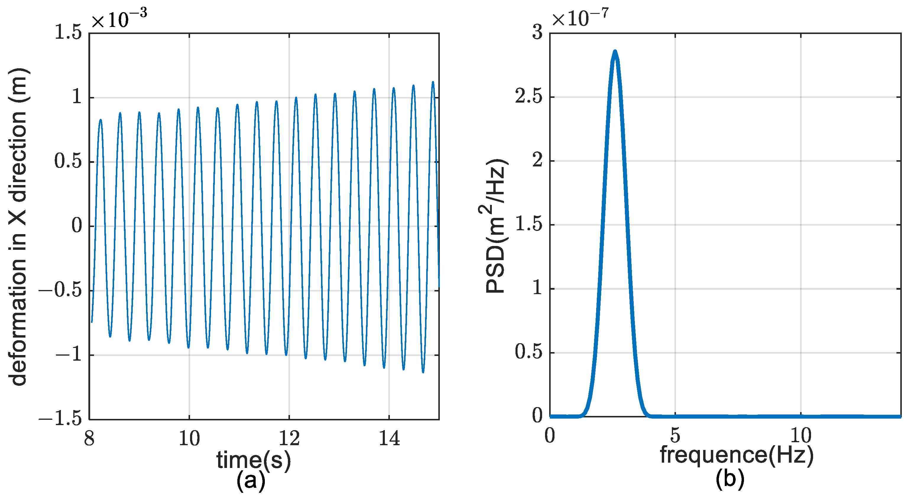
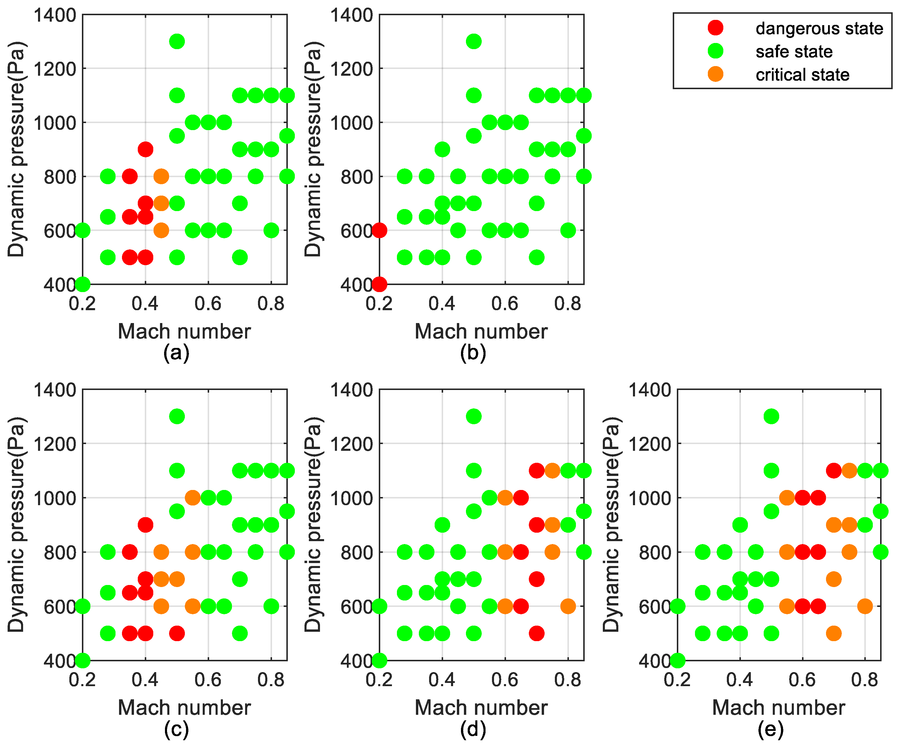
  • Through the analysis and calculation of multiple working conditions, the dangerous zone and safe zone as the fairing fell were obtained, which were consistent with the actual falling situation. When α 45 ° , the hazardous zone occurred at M a = 0.4 ; when α 45 ° , it was concentrated in the Mach number range of 0.6 to 0.8. At the same time, the influences according to dynamic pressure and Mach number were also analyzed.
  • According to the analysis, there is a risk of structural damage to the fairing as it falls. To suppress the vibration, a variety of possible methods were presented, such as enhancing the structural rigidity, flight attitude control, and opening the parachute at a high altitude. To verify the effectiveness of the method, a comprehensive method was used to calculate the vibration of the fairing during the descent. The fairing can land safely and avoid disintegration during the descent.

Author Contributions

Conceptualization, Z.W.; methodology, Z.W. and Z.Y.; software, Z.Y.; validation, Z.W. and Z.Y.; formal analysis, Z.Y.; writing—original draft preparation, Z.Y.; writing—review and editing, Z.W. and J.Z.; supervision, C.Y.; project administration, C.Y. All authors have read and agreed to the published version of the manuscript.

Funding

This research received no external funding.

Institutional Review Board Statement

Not applicable.

Informed Consent Statement

Not applicable.

Data Availability Statement

Not applicable.

Conflicts of Interest

The authors declare no conflict of interest.

Nomenclature

F C Vector of convective flux F V Vector of convective flux
p Pressure ρ Density
v Velocity vector T Temperature
E Total energy per unit mass k Thermal conductivity coefficient
τ ¯ Viscous stress tensor M Mass matrix
C Damping matrix K Stiffness matrix
ϕ Natural mode of the model z Displacement vector
f Load I ( n × n ) Identity matrix
Ω Diagonal matrix ω Frequency of the mode
Δ x i Displacement of the node m Number of iterations
MaMach number α Angle of attack
p ¯ Dynamic pressureUFlow speed
D DiameterLLength
μ Kinematic viscosity m * Non-dimensional mass
R e Reynolds number U r Reduced velocity
q Generalized displacement F Generalized force
V t Contravariant velocity of the face of a control volume
V r Contravariant velocity relative to the motion of the grid
n Outward-facing unit normal vector of dS
n i Number of nodes adjacent to node i
k i j Spring constant between the given node and adjacent nodes

Abbreviations

CFDComputational fluid dynamics
FSIFluid–structure interaction
CSDComputational structural dynamics
ROMReduced-order model
RANSReynolds-averaged Navier–stokes
DOFDegree of freedom
TPSThin Plate Spline
UDFUser-defined function

References

  1. Versiani, T.D.S.S.; Silvestre, F.J.; Neto, A.B.G.; Rade, D.A.; Silva, R.; Donadon, M.V.; Bertolin, R.M.; Silva, G.C. Gust load alleviation in a flexible smart idealized wing. Aerosp. Sci. Technol. 2019, 86, 762–774. [Google Scholar] [CrossRef]
  2. Shi, Y.; Wan, Z.Q.; Wu, Z.G.; Yang, C. Nonlinear unsteady aerodynamics reduced order model of airfoils based on algorithm fusion and multifidelity framework. Int. J. Aerosp. Eng. 2021, 2021, 4368104. [Google Scholar] [CrossRef]
  3. Dai, Y.T.; Wu, Y.; Yang, C.; Huang, G.J.; Huang, C. Numerical study on gust energy harvesting with an efficient modal based fluid-structure interaction method. Aerosp. Sci. Technol. 2021, 116, 106819. [Google Scholar] [CrossRef]
  4. Abdullah, N.A.; Curiel-Sosa, J.L.; Akbar, M. Aeroelastic assessment of cracked composite plate by means of fully coupled finite element and Doublet Lattice Method. Compos. Struct. 2018, 202, 151–161. [Google Scholar] [CrossRef]
  5. Omran, A.; Newman, B. Full envelope nonlinear parameter-varying model approach for atmospheric flight dynamics. J. Guid. Control Dyn. 2012, 35, 270–283. [Google Scholar] [CrossRef]
  6. Ruiz, C.; Acosta, J.Á.; Ollero, A. Aerodynamic reduced-order Volterra model of an ornithopter under high-amplitude flapping. Aerosp. Sci. Technol. 2022, 121, 107331. [Google Scholar] [CrossRef]
  7. Wu, T.; Kareem, A. A nonlinear analysis framework for bluff-body aerodynamics: A Volterra representation of the solution of Navier-Stokes equations. J. Fluids Struct. 2015, 54, 479–502. [Google Scholar] [CrossRef]
  8. Torregrosa, A.J.; Gil, A.; Quintero, P.; Cremades, A. A reduced order model based on artificial neural networks for nonlinear aeroelastic phenomena and application to composite material beams. Compos. Struct. 2022, 295, 115845. [Google Scholar] [CrossRef]
  9. Liu, Y.; Xie, C.C.; Yang, C.; Cheng, J.L. Gust response analysis and wind tunnel test for a high-aspect ratio wing. Chin. J. Aeronaut. 2016, 29, 91–103. [Google Scholar] [CrossRef] [Green Version]
  10. Kousen, K.A. Limit cycle phenomena in computational transonic aeroelasticity. J. Aircr. 1994, 31, 1257–1263. [Google Scholar] [CrossRef]
  11. Hallissy, B.; Cesnik, C. High-fidelity aeroelastic analysis of very flexible aircraft. In Proceedings of the 52nd AIAA/ASME/ASCE/AHS/ASC Structures, Structural Dynamics and Materials Conference, Denver, CO, USA, 4–7 April 2011. [Google Scholar]
  12. Mian, H.H.; Wang, G.; Ye, Z. Numerical investigation of structural geometric nonlinearity effect in high-aspect-ratio wing using CFD/CSD coupled approach. J. Fluids Struct. 2014, 49, 186–201. [Google Scholar] [CrossRef]
  13. Ilie, M. A fully-coupled CFD/CSD computational approach for aeroelastic studies of helicopter blade-vortex interaction. Appl. Math. Comput. 2019, 347, 122–142. [Google Scholar] [CrossRef]
  14. Aprovitola, A.; Dyblenko, O.; Pezzella, G.; Viviani, A. Aerodynamic analysis of a supersonic transport aircraft at low and high speed flow conditions. Aerospace 2022, 9, 411. [Google Scholar] [CrossRef]
  15. Franzmann, C.; Leopold, F.; Mundt, C. Low-interference wind tunnel measurement technique for pitch damping coefficients at transonic and low supersonic Mach numbers. Aerospace 2022, 9, 51. [Google Scholar] [CrossRef]
  16. Zhong, Q.; Fan, Y.H.; Wu, W.B. A switching-based control method for the fairing separation control of axisymmetric hypersonic vehicles. Aerospace 2022, 9, 132. [Google Scholar] [CrossRef]
  17. Tsutsumi, S.; Takaki, R.; Takama, Y.; Imagawa, K.; Nakakita, K.; Kato, H. Hybrid LES/RANS Simulations of Transonic Flowfield Around a Rocket Fairing. In Proceedings of the 30th AIAA Applied Aerodynamics Conference, New Orleans, LA, USA, 25–28 June 2012. [Google Scholar]
  18. Morshed, M.M.M.; Hansen, C.H.; Zander, A.C. Prediction of Acoustic Loads on a Launch Vehicle Fairing During Liftoff. J. Spacecr. Rocket. 2013, 50, 159–168. [Google Scholar] [CrossRef]
  19. Tatsukawa, T.; Nonomura, T.; Oyama, A.; Fujii, K. Multi-Objective Aeroacoustic Design Exploration of Launch-Pad Flame Deflector Using Large-Eddy Simulation. J. Spacecr. Rocket. 2016, 53, 751–758. [Google Scholar] [CrossRef]
  20. Sunil, K.; Johri, I.; Priyadarshi, P. Aerodynamic Shape Optimization of Payload Fairing Boat Tail for Various Diameter Ratios. J. Spacecr. Rocket. 2022, 59, 1135–1148. [Google Scholar] [CrossRef]
  21. Cheng, Y.; Li, D.C.; Xiang, J.W.; Da Ronch, A. Energy harvesting performance of plate wing from discrete gust excitation. Aerospace 2019, 6, 37. [Google Scholar] [CrossRef] [Green Version]
  22. Bekemeyer, P.; Timme, S. Flexible aircraft gust encounter simulation using subspace projection model reduction. Aerosp. Sci. Technol. 2019, 86, 805–817. [Google Scholar] [CrossRef]
  23. Wang, N.K. Fluid Structure Coupling Analysis of Non-Streamline Construction. Master’s Thesis, Beihang University, Beijing, China, 2020. [Google Scholar]
  24. Guo, T.; Lu, D.; Lu, Z.; Zhou, D.; Lyu, B.; Wu, J. CFD/CSD-based flutter prediction method for experimental models in a transonic wind tunnel with porous wall. Chin. J. Aeronaut. 2020, 33, 3100–3111. [Google Scholar] [CrossRef]
  25. Barakos, G.N.; Fitzgibbon, T.; Kusyumov, A.N.; Kusyumov, S.A.; Mikhailov, S.A. CFD simulation of helicopter rotor flow based on unsteady actuator disk model. Chin. J. Aeronaut. 2020, 33, 2313–2328. [Google Scholar] [CrossRef]
  26. Singh, S.P.; Mittal, S. Vortex-induced oscillations at low Reynolds numbers: Hysteresis and vortex-shedding modes. J. Fluids. Struct. 2005, 20, 1085–1104. [Google Scholar] [CrossRef]
  27. Huang, J.L. Study on Flow-Induced Vibrations of Two Tandem-Arranged Circular Cylinders in Laminar Flow with Low Reynolds Number. Master’s Thesis, Tianjin University, Tianjin, China, 2012. [Google Scholar]
  28. Wang, M. Numerical Investigation on Vortex-Induced Vibrations of the Tandem Wavy Cylinders. Master’s Thesis, Wuhan University of Technology, Wuhan, China, 2016. [Google Scholar]
  29. Draft Environmental Assessment for Issuing a Reentry License to SpaceX for Landing the Dragon Spacecraft in the Gulf of Mexico. Available online: http://34.196.180.244/2018/04/12/details-spacex-fairing-drogue-parachute-recovery-efforts/ (accessed on 16 November 2022).
Figure 1. Schematic of a typical fairing. (a) Configuration I and (b) Configuration II.
Aerospace 09 00741 g001
Figure 2. Flowchart of CFD–CSD coupling.
Aerospace 09 00741 g002
Figure 3. Definitions of the angle of attack and coordinates.
Aerospace 09 00741 g003
Figure 4. Structural grid and monitoring point (red star).
Aerospace 09 00741 g004
Figure 5. Mode shapes and frequencies. (a) First-order mode, 2.2 Hz, (b) second-order mode, 5.8 Hz, (c) third-order mode, 9.1 Hz, and (d) fourth-order mode, 11.5 Hz.
Aerospace 09 00741 g005
Figure 6. Fluid mesh. (a) Global mesh. (b) Mesh on the surface of the fairing.
Aerospace 09 00741 g006
Figure 7. Generalized displacement of the three grid systems. (a) First-order mode, (b) second-order mode, (c) third-order mode, and (d) fourth-order mode.
Aerospace 09 00741 g007
Figure 8. Physical model of the vortex-induced vibration of a single cylinder.
Aerospace 09 00741 g008
Figure 9. Comparison of the results of the simulations with those reported in the literature Singh et al. [26], Huang et al. [27], Wang et al. [28].
Aerospace 09 00741 g009
Figure 10. Curves of the generalized displacement–time response ( M a = 0.5 , p ¯ = 700   Pa ). (a) First-order mode, (b) second-order mode, (c) third-order mode, and (d) fourth-order mode.
Aerospace 09 00741 g010
Figure 11. Curves of the generalized force–time response ( M a = 0.5 , p ¯ = 700   Pa ). (a) First-order mode, (b) second-order mode, (c) third-order mode, and (d) fourth-order mode.
Aerospace 09 00741 g011
Figure 12. Curves of the generalized displacement–time response ( M a = 0.6 , p ¯ = 1000   Pa ). (a) First-order mode, (b) second-order mode, (c) third-order mode, and (d) fourth-order mode.
Aerospace 09 00741 g012
Figure 13. Curves of the generalized force–time response ( M a = 0.6 , p ¯ = 1000   Pa ). (a) First-order mode, (b) second-order mode, (c) third-order mode, and (d) fourth-order mode.
Aerospace 09 00741 g013
Figure 14. Spectral analysis of the X displacement of the monitoring point. (a) Deformation in the X direction. (b) PSD of deformation in the X direction.
Aerospace 09 00741 g014
Figure 15. Diagram of deformation of the fairing in one cycle: (a) 1/9 T, (b) 2/9 T, (c) 3/9 T, (d) 4/9 T, (e) 5/9 T, (f) 6/9 T, (g) 7/9 T, (h) 8/9 T, and (i) T.
Aerospace 09 00741 g015aAerospace 09 00741 g015b
Figure 16. Vibration attenuation.
Aerospace 09 00741 g016
Figure 17. The logarithmic decay rate of the generalized displacement varies with varying Mach numbers ( p ¯ = 600   Pa , α = 90 ° ).
Aerospace 09 00741 g017
Figure 18. Variations in the logarithmic decay rate of generalized displacement with the Mach number ( p ¯ = 800   Pa , α = 45 ° ).
Aerospace 09 00741 g018
Figure 19. Variations in the logarithmic decay rate of generalized displacement with the dynamic pressure ( M a = 0.4 , α = 45 ° ).
Aerospace 09 00741 g019
Figure 20. Variations in the logarithmic decay rate of generalized displacement with the dynamic pressure ( M a = 0.6 , α = 90 ° ).
Aerospace 09 00741 g020
Figure 21. Summary of the results of the calculation: (a) α = 0 , (b) α = 20 ° , (c) α = 45 ° , (d) α = 70 ° , and (e) α = 90 ° .
Aerospace 09 00741 g021
Figure 22. Curves of the generalized displacement time–response with shells of different thicknesses. (a) First-order mode, (b) second-order mode, (c) third-order mode, and (d) fourth-order mode.
Aerospace 09 00741 g022
Figure 23. Variations in the logarithmic decay rate of the generalized displacement with the thickness of the shell (the relative thickness is equal to the thickness divided by the initial thickness).
Aerospace 09 00741 g023
Figure 24. Control schemes implemented during the process of falling of the fairing.
Aerospace 09 00741 g024
Figure 25. Detailed situation of path one.
Aerospace 09 00741 g025
Figure 26. Variations in the logarithmic decay rate of the generalized displacement with path one.
Aerospace 09 00741 g026
Table 1. Material properties of each part of the fairing.
FairingYoung’s Modulus (Pa)Poisson’s RatioDensity (kg/m3)
Head 6.9 × 10 10 0.333200
Shell 1.5 × 10 10 0.332500
Table 2. Working conditions.
Working ConditionDynamic Pressure (Pa)Mach NumberTemperature (K)
17000.5218.6
210000.6220
Table 3. The number of elements in the three grid systems.
GridElementsMinimum Volume (m3)
Fine2,362,564 4.8 × 10 8
Baseline1,876,113 5.1 × 10 8
Coarse1,517,761 5.5 × 10 8
Table 4. Advantages and disadvantages of the three methods.
MethodAdvantagesDisadvantages
Increasing structural rigidityEasy to alterIncreased launch cost
Increased weight
Attitude controlLight in added weightComplicated to alter
Opening the parachute at high altitudeRelatively light in added weightIncreased certain launch cost
Relatively complicated to alter
Publisher’s Note: MDPI stays neutral with regard to jurisdictional claims in published maps and institutional affiliations.

